


 Abstract
 HTML
HTML Reference
 Related
 PDF
PDF


-
Very high energy (VHE, >100 GeV)
$ \gamma $ -rays open a crucial window for exploring the non-thermal phenomena in the Universe in the most extreme environments. Their detailed observation allows to comprehend the puzzles in modern astrophysics and cosmology, particularly of the origin of Galactic and extragalactic cosmic rays, the acceleration and radiation process in violent environments like supernova remnant (SNR) shocks, active galactic nuclei outflows or pulsar winds. Besides, they may contribute to cosmological issues by constraining the annihilation cross-section of dark matter like WIMPs and searching for Lorentz invariance violation.The astrophysical
$ \gamma $ -ray sky is usually decomposed into the individually detected sources and the diffuse$ \gamma $ -ray emission. The former, including point sources and extended sources, contain many different types: Galactic sources like SNRs, pulsar wind nebulae (PWN), binaries etc., and extragalactic sources like AGN. Galactic cosmic rays (GCRs) are accelerated by shock waves generated in SNR [1]; electrons gain energy effectively at the termination shock of PWN where the pulsar wind is terminated by the surrounding gas, emitting TeV$ \gamma $ -rays via the inverse Compton scattering [2-3]. Beyond our Galaxy, almost all known TeV$ \gamma $ -ray sources are AGN and their$ \gamma $ -ray emissions are thought to originate from one or multiple regions of particle acceleration in the jets. The diffuse$ \gamma $ -ray emission is mainly attributed to the interactions of CR electrons and nuclei with interstellar gas [4] and photon fields in the Galactic plane, and provides a key insight into the character of propagation of CRs in the Galaxy.Various techniques have been developed to detect very high energy (VHE)
$ \gamma $ -rays. The Fermi Large Area Telescope (Fermi-LAT), one of the space-borne observatories, has found thousands of$ \gamma $ -ray sources in the GeV band. However, due to their limited effective area and low$ \gamma $ -ray flux at higher energies, the space detectors are insensitive compared with the ground-based observatories in the VHE range. There are two main techniques used in ground observatories. One is the imaging atmospheric Cherenkov telescope (IACT), such as H.E.S.S. [5], MAGIC [6] and VERITAS [7], which observe the Cherenkov light emitted by secondary particles generated in air showers. The other is the extensive air shower (EAS) array technique, like Tibet AS$ \gamma $ [8] and ARGO-YBJ [9], where secondary particles are detected at the ground level. The use of the water Cherenkov technique for gamma-ray observations was developed by Milagro [10], where secondary particles ($ e^{\pm} $ and muons) pass through pure water. This technique allows better photon/hadron discrimination compared with EAS arrays. While it does not have the excellent angular and energy resolution and the strong background-rejecting capability of IACT, the water Cherenkov detector exhibits a high duty cycle and a wide field of view (FOV) with moderate angular resolution and background rejection ability. Therefore, it is suitable for monitoring the whole sky and observing extended sources.HAWC has reported the detection of at least 39 sources in the Northern sky survey [11]. Given its larger effective area, WCDA will provide an improvement with respect to the previous and current experiments like HAWC. The prospects of WCDA to search for
$ \gamma $ -rays are presented in this paper. We introduce WCDA in Sec. 2, and describe the properties of the sources and the simulation process in Sec. 3. The analysis method, namely the all-sky method, is presented in Sec. 4. Finally, we predict the significance of the detection of the sources and the diffuse$ \gamma $ -rays in Sec. 5. -
WCDA detects showers in the primary energy range from 100 GeV to 20 TeV, and constitutes an important part of LHAASO, located on the Daocheng site, Sichuan province, P.R. China (
$ 29^{\circ}21^\prime31^{\prime\prime} $ N,$ 100^{\circ}08^{\prime}15^{\prime\prime} $ E), at an altitude of 4410 m. The original array covers 90,000$ {\rm m}^2 $ as reported in [12], which is divided into 4 subarrays with a size of 150 m$ \times $ 150 m. Each subarray contains 900 detector units measuring 5 m$ \times $ 5 m. One upward-facing 8-inch photomultiplier tube (PMTs) is anchored at the center of the unit, at its bottom. The prospects of WCDA reported in this paper are based on this original configuration. The design has been modified and we discuss the effect of the differences on our result in Sec. 6.The simulation based on the original design mentioned above was reported in [13, 14]. The simulation used CORSIKA6735 [15] to simulate the cascade processes of
$ \gamma $ -rays and cosmic rays in the atmosphere. A program based on GEANT4 [16] was employed to study the detector responses. The simulation tracked the Crab Nebula, a source typically used as a "standard candle" in VHE$ \gamma $ -ray astronomy, to generate$ \gamma $ -ray and CRs events. We call this simulation the Crab-centered simulation. We adopt the Crab spectrum measured by HEGRA [17], and the spectra of cosmic rays follow the Hörandel model [18]. The direction of the simulated events were reconstructed by fitting the shower fronts. Based on this simulation, we selected a data set to study the properties of WCDA, mainly the effective area, point-spread function (PSF), and photon/hadron discrimination. Three principles for data selection were adopted: first, the reconstructed zenith angle has to be less than$ 45^\circ $ ; second, the number of triggered detectors needs to be more than 128; third, the "compactness" [19, 20] should be larger than 14.4. The compactness is defined as$ n{\rm PMTs}/Cx{\rm PE}_{45} $ , where$ Cx{\rm PE}_{45} $ is the maximal energy deposition of photo-electrons (PEs) recorded by one PMT beyond a radius of 45 meters from the reconstructed air shower core;$ n{\rm PMTs} $ denotes the number of triggered PMTs. The median energy in the data set is around 1 TeV. After obtaining these properties, the detection ability of WCDA to other sources is estimated from a fast simulation described in Section 3.The effective area for
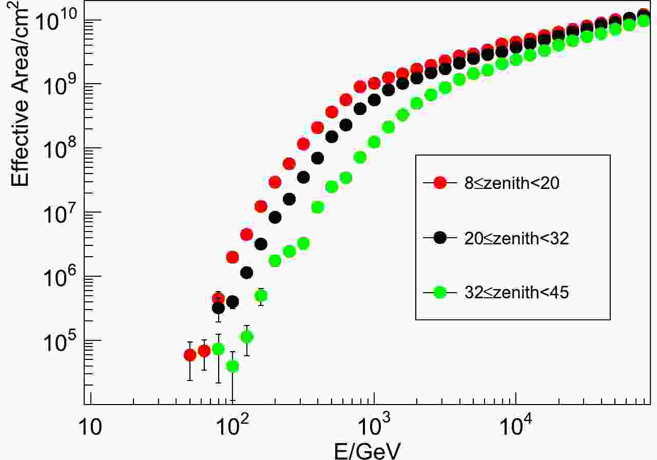
$ \gamma $ -rays as a function of energy and zenith angle is shown in Fig. 1, and for CRs in Fig. 2. The effective area for$ \gamma $ -rays is used to generate the$ \gamma $ signals from different sources, and the effective area for cosmic rays is used to produce the background, as explained in Section 3.
Figure 1. (color online)
$\gamma$ -ray effective area of WCDA as a function of energy and zenith angle. Red dots denote the effective area in$8^\circ - 20^\circ$ zenith angle range; black dots denote the effective area in$20^\circ - 32^\circ$ zenith angle range; green dots denote the effective area in$32^\circ - 45^\circ$ zenith angle range.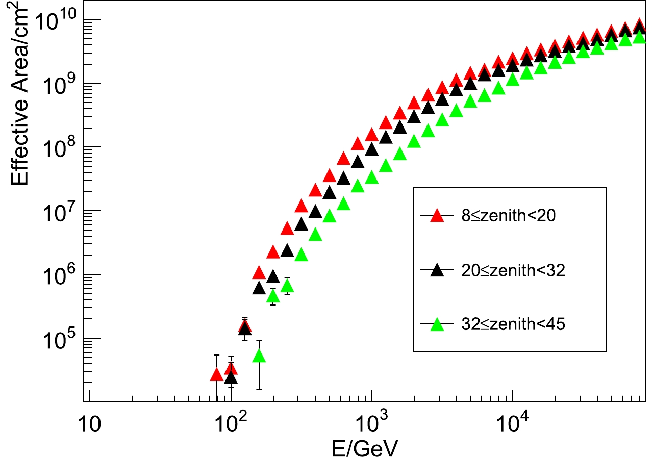
Figure 2. (color online) Cosmic-ray effective area of WCDA as a function of energy and zenith angle. Red dots denote the effective area in
$8^\circ - 20^\circ$ zenith angle range; black dots denote the effective area in$20^\circ - 32^\circ$ zenith angle range; green dots denote the effective area in$32^\circ - 45^\circ$ zenith angle range.PSF gives the difference between the original direction and the reconstructed direction after accounting for the detector response. PSF for the selected data set is shown in Fig. 3. The direction of the
$ \gamma $ -ray signals from the sources are smeared with this function. The blue dashed line in Fig. 3 shows the PSF of WCDA, and the red line shows the PSF for our fast simulation. The two lines agree which demonstrates that our fast simulation spreads the signals from the$ \gamma $ sources according to the PSF of WCDA. PSF convolutes the energy bins. We analyze only one energy bin with the median energy of 1 TeV, so that one specific PSF is used. Due to the PSF of WCDA,$ \gamma $ -ray signals from a point source follow a central symmetric distribution around the source. We integrate the signal and cosmic-ray background counts within a circular disc centered on a sky position. The optimal disc radius is found by maximizing the figure of merit$ S/\sqrt{B} $ where S is the number of signal counts, and B of the background counts. The best signal-to-noise ratio occurs at$ 0.56^\circ $ , denoted by the red vertical line in Fig. 3. Therefore, the angular smoothing radius is$ 0.56^\circ $ .
Figure 3. (color online) PSF of WCDA. The blue dashed line is the PSF derived from the selected data set. The red solid line is the PSF for our fast simulation. The two lines agree which ensures the reliability of our fast simulation. The red vertical line denotes the optimized angular radius (
$0.56^\circ$ ) with the best signal-to-noise ratio.WCDA uses the compactness parameter to discriminate
$ \gamma $ -rays from cosmic rays. Statistically, the compactness distributions of$ \gamma $ -rays and cosmic rays are different, as shown in Fig. 4. The compactness of$ \gamma $ -ray showers is smaller than of cosmic rays, because secondary muons are more likely to deposit energy in PMTs far from the air shower core, and they mainly originate from hadronic cosmic ray interactions in the atmosphere. We quantify the performance of the photon/hadron rejection method by calculating its Q factor defined as$ Q = \frac{\eta_{\gamma}}{\sqrt{\eta_{cr}}} $ , where$ \eta_{\gamma} $ and$ \eta_{cr} $ are the efficiencies of simulated$ \gamma $ -rays and cosmic rays for a compactness greater than a certain value. We scan for the maximal Q factor by varying the compactness as shown in Fig. 5. For this data set, the optimized photon/hadron discrimination is a compactness$ >14.4 $ , with the efficiency of$ \gamma $ -rays ($ \eta_{\gamma} $ ) and CRs ($ \eta_{cr} $ ) of 40% and 0.27%, respectively.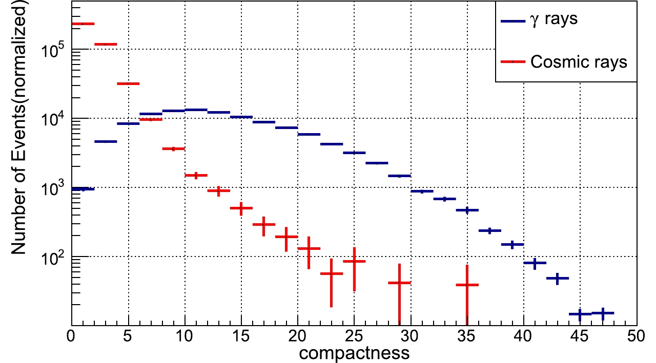
Figure 4. (color online) Compactness distribution of
$\gamma$ -rays (red line) and cosmic rays (blue line).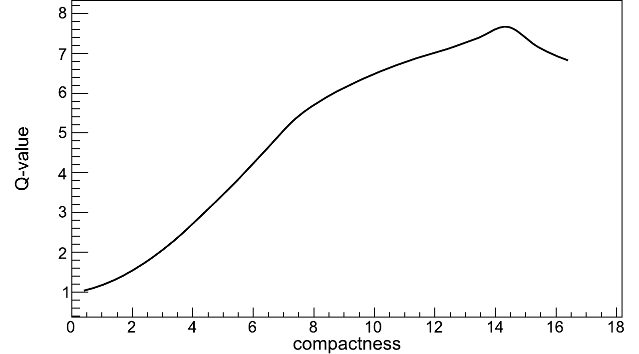
Figure 5. Q factor as a function of the compactness.
-
Apart from the Crab-centered simulation, we performed a fast simulation of the array exposure across its field of view (FOV) to calculate the detection significance of all sources in TeVCat①. In this work, the FOV of WCDA is defined as the portion of the sky with a zenith angle
$ \leqslant 45^{\circ} $ . We project this FOV in local coordinates (zenith and azimuth), in which the zenith angle ($ \theta $ ) is binned in$ 0.08^{\circ} $ bins and the azimuth ($ \phi $ ) is binned in$ \frac{0.08^{\circ}}{\sin\theta} $ bins, so that each window contains the same steradian units for the solid angle$ \Omega = 1.95\times10^{-6} $ . Also, the sidereal day is divided into 3600 time bins, in other words, one day contains 3600 maps with an exposure time of 24 seconds. The predicted number of cosmic rays or diffuse$ \gamma $ rays in a window$ (t,\theta,\phi) $ is calculated as$ N_{i}(t,\theta,\phi) = \eta_{i}\int_{E} \phi_{i}(E)A_{i}(\theta,E)\Omega\, {\rm d}E\delta t, $

(1) where
$ \Omega $ is the solid angle in steradian units, and$ \delta t $ is the period of one map, that is 24 seconds. In the case when i stands for CRs,$ A_{i}(\theta,E) $ is the differential effective area of cosmic rays,$ \phi_{i}(E) $ is the cosmic ray spectrum [21], and$ \eta_{i} $ is the efficiency of CRs which passed the photon/hadron criterion. When i stands for the diffuse$ \gamma $ -rays, these parameters are the values for$ \gamma $ rays. We take the diffuse$ \gamma $ -rays spectra from Ref. [22]. We track every source located in FOV and calculate the number of$ \gamma $ -ray events from each source. The predicted number in a window$ (t,\theta,\phi) $ is calculated as$ N_{\gamma}(t,\theta,\phi) = \eta_{\gamma}\int_{E} \phi(E)_{\gamma}A_{\gamma}(\theta,E)\, {\rm d}E\delta t . $

(2) The meaning of each parameter is the same as in Eq. (1), but represent
$ \gamma $ -rays excluding the solid angle. The spectra of the sources used are listed in Tables 1, 2, 3, 4. The spectra of sources are described by a power law with a fixed index$ \phi(E) = N_{0}(\frac{E}{E_{0}})^{-\beta} $ , where$ N_0 $ is the differential flux at$ E_0 $ , and$ \beta $ is the spectral index. If the spectra of the sources are measured with an exponential energy cut, they are in the form$ \phi(E) = (\frac{E}{E_{0}})^{-\beta}{\rm e}^\frac{-E}{E_{\rm cut}} $ , where$ E_{\rm cut} $ is the exponential cutoff energy of the sources. For the extended sources, the extension is determined by fitting the excess map with a two-dimensional (2D) Gaussian convoluted with PSF [34]. Therefore, we use the 2D Gaussian model to produce the morphologies of the extended sources. The parameters for each source are listed in Tables 1,2,3,4.TeVCat Name ${\rm R.A.}/(^\circ)$ 

${\rm Dec.}/(^\circ)$ 

$\sigma$ 

$N_0/{\rm (TeV^{-1 }cm^{-2}s^{-1})}$ 

$E_{0}/{\rm TeV}$ 

$\beta$ 

${\rm Extension}/(^\circ)$ 

Ref. LS I +61303 40.14 61.26 9.4 $1.80\times 10^{-12}$ 

1 2.34 − [23] HESS J1912+101 288.20 10.15 9.7 $3.66\times 10^{-14}$ 

7 2.64 0.7 [11] W51 290.73 14.19 10.0 $2.61\times 10^{-14}$ 

7 2.51 0.9 [11] ARGO J2031+ $4157^a$ 

307.8 42.50 67.5 $3.50\times 10^{-9}$ 

0.1 2.16 2 [9] Cassiopeia A 350.81 58.81 7.2 $1.45\times 10^{-12}$ 

1 2.75 − [24] a: Identified as the counterpart of the Cygnus Cocoon at TeV energies, whose spectrum exhibits an exponential cutoff at 40 TeV. Table 1. Significance of superbubbles, SNRs, Shells, Binaries.
$\sigma$ is the significance of the sources,$N_0$ the differential flux at$E_0$ ,$\beta$ the spectral index, and Extension is the extended angular radius (in degrees) assuming the two-dimensional Gaussian model.TeVCat Name ${\rm R.A.}/(^\circ)$ 

${\rm Dec.}/(^\circ)$ 

$\sigma$ 

$N_0/{\rm (TeV^{-1 }cm^{-2}s^{-1})}$ 

$E_{0}/{\rm TeV}$ 

$\beta$ 

${\rm Extension}/(^\circ)$ 

Ref. Crab 83.63 22.01 307.7 $1.85\times 10^{-13}$ 

7 2.58 − [11] Geminga 98.12 17.37 10.7 $4.87\times 10^{-14}$ 

7 2.23 2 [11] HESS J1831-098 277.85 −9.90 9.4 $9.58\times 10^{-14}$ 

7 2.64 0.9 [11] TeV J1930+188 292.63 18.87 23.9 $9.80\times 10^{-15}$ 

7 2.74 − [11] Table 2. Significance of PWN.
$\sigma$ is the significance of the sources,$N_0$ the differential flux at$E_0$ ,$\beta$ the spectral index, and Extension is the extended angular radius (in degrees) assuming the two-dimensional Gaussian model.TeVCat Name ${\rm R.A.}/(^\circ)$ 

${\rm Dec.}/(^\circ)$ 

$\sigma$ 

$N_0/{\rm (TeV^{-1 }cm^{-2}s^{-1})}$ 

$E_{0}/{\rm TeV}$ 

$\beta$ 

$E_{\rm cut}/{\rm TeV}$ 

Ref. S3 0218+ $35^f$ 

35.27 35.94 6.4 $2.00\times 10^{-9}$ 

0.1 3.8 − [25] VER J0521+211 80.44 21.21 12.4 $1.99\times 10^{-11}$ 

0.4 3.44 − [26] RGB J0710+591 107.61 59.15 5.8 $9.20\times 10^{-13}$ 

1 2.69 − [27] Markarian 421 166.08 38.19 236.8 $2.82\times 10^{-11}$ 

1 2.21 5.4 [11] 1ES 1215+ $303^f$ 

184.45 30.10 5.2 $2.30\times 10^{-11}$ 

0.3 3.6 − [28] 1ES 1218+304 185.36 30.19 17.9 $1.40\times 10^{-12}$ 

1 3.13 − [29] W Comae 185.38 28.23 11.1 $2.00\times 10^{-11}$ 

0.4 3.81 − [30] M 87 187.70 12.40 6.8 $7.70\times 10^{-12}$ 

0.3 2.21 − [6] H 1426+428 217.14 42.67 61.6 $4.37\times 10^{-12}$ 

1 3.54 − [31] Markarian 501 253.47 39.76 47.5 $4.40\times 10^{-12}$ 

1 1.6 5.7 [11] 1ES 1959+650 300.00 65.15 28.8 $6.12\times 10^{-12}$ 

1 2.54 − [32] RGB J2056+ $496^f$ 

314.18 49.67 9.7 $1.15\times 10^{-11}$ 

0.4 2.77 − [33] 1ES 2344+514 356.77 51.71 19.2 $2.65\times 10^{-12}$ 

0.91 2.46 − [7] f: The spectrum of this source is in a flare state. Table 3. Significance of AGN.
$\sigma$ is the significance of sources,$N_0$ the differential flux at$E_0$ ,$\beta$ the spectral index, and$E_{\rm cut}$ is the exponential cutoff energy of the sources.TeVCat Name ${\rm R.A.}/(^\circ)$ 

${\rm Dec.}/(^\circ)$ 

$\sigma$ 

$N_0/{\rm (TeV^{-1 }cm^{-2}s^{-1})}$ 

$E_{0}/{\rm TeV}$ 

$\beta$ 

${\rm Extension}/(^\circ)$ 

Ref. 2HWC J1309-054 197.31 −5.49 7.8 $1.23\times 10^{-14}$ 

7 2.55 − [11] HESS J1813-126 273.34 −12.69 5.9 $2.74\times 10^{-14}$ 

7 2.84 − [11] 2HWC J1825-134 276.46 −13.40 8.0 $2.49\times 10^{-13}$ 

7 2.56 0.9 [11] 2HWC J1829+070 277.34 7.03 11.1 $8.10\times 10^{-15}$ 

7 2.69 − [11] 2HWC J1837-065 279.36 −6.58 35.1 $3.41\times 10^{-13}$ 

7 2.66 2 [11] 2HWC J1844-032 281.07 −3.25 10.8 $9.28\times 10^{-14}$ 

7 2.51 0.6 [11] 2HWC J1852+013 283.01 1.38 27.8 $1.82\times 10^{-14}$ 

7 2.9 − [11] MAGIC J1857.6+0297 284.40 2.97 9.2 $6.10\times 10^{-12}$ 

1 2.39 0.1 [34] HESS J1858+020 284.58 2.09 8.3 $6.00\times 10^{-13}$ 

1 2.17 0.08 [34] 2HWC J1902+048 285.51 4.86 31.1 $8.30\times 10^{-15}$ 

7 3.22 − [11] 2HWC J1907+084 286.79 8.50 31.6 $7.30\times 10^{-15}$ 

7 3.25 − [11] MGRO J1908+06 286.98 6.27 10.9 $8.51\times 10^{-14}$ 

7 2.33 0.8 [11] 2HWC J1914+117 288.68 11.72 20.5 $8.50\times 10^{-15}$ 

7 2.83 − [11] 2HWC J1921+131 290.30 13.13 20.9 $7.90\times 10^{-15}$ 

7 2.75 − [11] 2HWC J1928+177 292.15 17.78 20.1 $1.07\times 10^{-14}$ 

7 2.6 − [35] 2HWC J1938+238 294.74 23.81 26.3 $7.40\times 10^{-15}$ 

7 2.96 − [11] 2HWC J1953+294 298.26 29.48 21.8 $8.30\times 10^{-15}$ 

7 2.78 − [11] 2HWC J1955+285 298.83 28.59 7.8 $5.70\times 10^{-15}$ 

7 2.4 − [11] 2HWC J2006+341 301.55 34.18 119.6 $9.60\times 10^{-15}$ 

7 2.64 − [11] VER J2019+407 305.02 40.76 22.9 $1.50\times 10^{-12}$ 

1 2.37 0.23 [36] Table 4. Significance of unidentified sources (UID).
$\sigma$ is the significance of sources,$N_0$ the differential flux at$E_0$ ,$\beta$ the spectral index, and Extension is the extended angular radius (in degrees) assuming the two-dimensional Gaussian model. -
Since the events in each pixel contain the
$ \gamma $ -ray signals and the background CRs, the key point is to estimate the background properly and test whether there is a significant excess. We use the All-Sky analysis method to estimate the background events, which has been successfully used in the Tibet AS$ \gamma $ experiment [37].The detection efficiency largely depends on the zenith angle, because more inclined events pass through a greater atmospheric depth. However, the efficiency in one zenith belt is independent of the azimuth angle given that WCDA is sitting almost in a horizontal plane. In the estimate of the background events in a window in the fast simulation, the window is called the "on-source window", and the sideband windows in the same zenith angle belt are referred to as the "off-source windows". The background events in the "on-source window" are estimated from the average number of "off-source windows". FOV in equatorial coordinates is divided into small pixels which measure
$ 0.1^\circ \times 0.1^\circ $ , and each window marked as$ (t,\theta,\phi) $ in the fast simulation corresponds to a pixel marked as$ (i,j) $ in equatorial coordinates. The number of events in the on-source window is denoted as$ N_{t,\theta,\phi} $ and the relative intensity as$ I_{i,j} $ , the number of events in the$ \phi' $ -th off-source window as$ N_{t,\theta,\phi'} $ and the relative intensity as$ I_{i',j'} $ , and we have$ \frac{N_{t,\theta,\phi}}{I_{i,j}} = <\frac{N_{t,\theta,\phi'}}{I_{i',j'}}> $ . For the FOV of WCDA,$ \tilde{\chi}^2 = \sum\limits_{i,j}^{}\left( \bigg(\dfrac{N_{t,\theta,\phi}}{I_{ij}} -\dfrac{1}{n_{\theta}-1} \displaystyle\sum_{\phi'}\dfrac{N_{t,\theta,\phi'}} {I_{i'j'}} \bigg) \bigg/ {\sigma_{t,\theta,\phi}}\right)^2 . $

(3) Here,
$ n_{\theta} $ represents the number of windows in the$ \theta $ zenith belt. We get the relative intensity$ I_{i,j} $ and the estimated error$ \delta I_{i,j} $ by minimizing$ \tilde{\chi}^2 $ . The background in each pixel is$ N_{bkg i,j} = \frac{N_{i,j}}{I_{i,j}} $ . The relative intensity gives the deviation in the number of events from the backgrounds expectation. The significance of deviation is calculated as$ \sigma = \frac{I_{i,j}-1}{\delta I_{i,j}} $ .In the fast simulation, the skymap contains
$ \gamma $ -rays from the sources and the diffuse emissions. However, the signal counts from the sources near the Galactic plane may have an underlying diffuse component. We adopt the likelihood ratio method to decompose the two components [11].$ {\cal{L}} = \ln \frac{{\cal{L}}({\rm signal\ model})}{{\cal{L}}({\rm Null{\ }model})} . $

In the analysis, the signal model considers the signal counts from two components,
$ M_{i,j} = $ $ N^{'}_{i,j} + N^{'}_f $ .$ N^{'}_{i,j} $ is the source contribution to the pixel$ (i,j) $ derived from the source flux and the detector response. The morphology of the point sources is described by PSF, and that of the extended sources can be characterized by the extended source shapes (2D Gaussian model) convoluted with PSF. To evaluate the maximum possible contribution of the diffuse emission to the source signal counts, we assume that$ N^{'}_f $ is a constant number for each pixel in a circular$ 3^\circ $ region of interest (ROI) centered on our source. Therefore, the signal likelihood is$ {\cal{L}}({\rm signal\; model})\! = \sum_{i,j} \ln P_{i,j}$ $\! (N_{i,j},N_{bkg i,j}\!+\!M_{i,j}) $ , where$ P_{i,j} $ is the Poisson probability of observing$ N_{i,j} $ counts given the expectation$ N_{bkg i,j}+M_{i,j} $ . As for the null model, the expectation only considers the background counts$ N_{bkg i,j} $ . We use the Minuit library [38] to maximize the likelihood ratio. -
The sensitivity of WCDA as function of declination is presented in Fig. 6, and the spectrum index is -2.62.
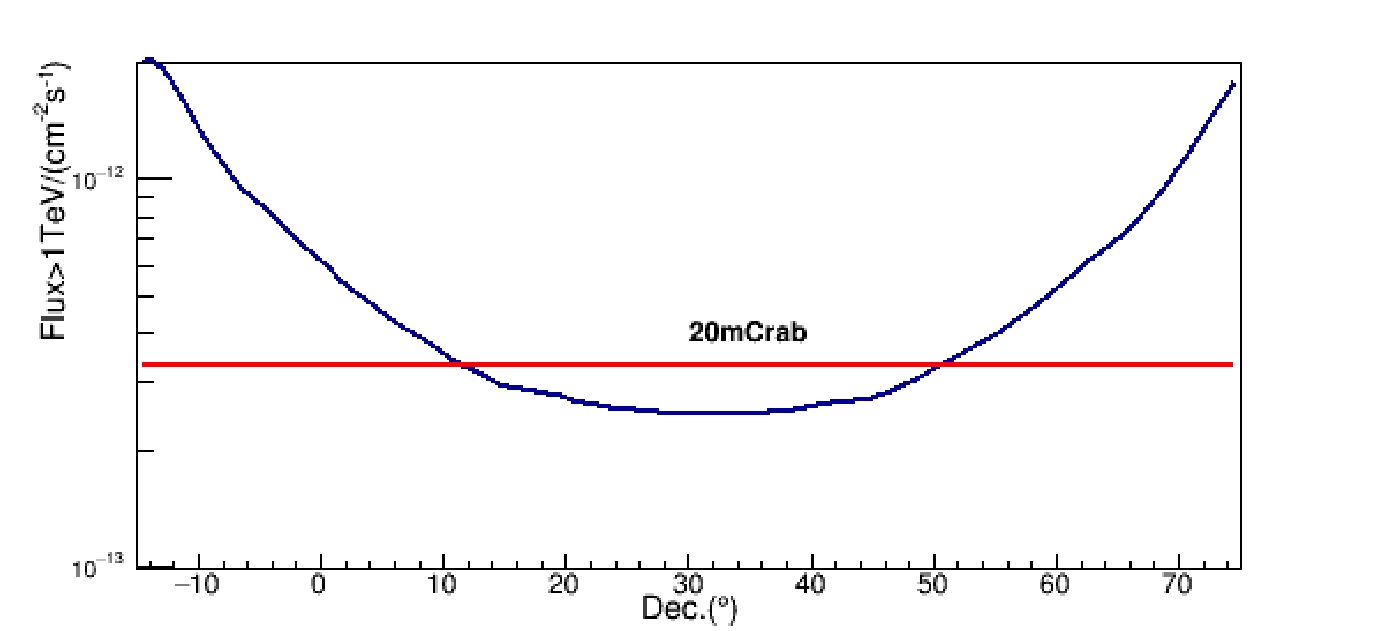
Figure 6. (color online) Sensitivity as function of declination.
The
$ \gamma $ -ray signals from the sources are based on the spectra in TeVCat, and the spectra of diffuse emissions are calculated by the spatially dependent diffusion model [22], which accounts well for the Galactic plane flux measured by Fermi-LAT [39]. Therefore, we use this model to calculate the spectra of diffuse$ \gamma $ -rays in the TeV range. In this model, two regions contribute to the diffuse volume, one is close to the Galactic disk called the inner halo, and the other is the outer halo. The turbulences in the inner halo originate from supernova explosions, while the turbulences in the outer halo are mainly generated by CRs themselves. Therefore, the energy spectra of turbulences in the inner halo are harder than in the outer halo while the diffusion is slower. In the outer halo, the diffusion coefficient is only rigidity dependent, while in the inner halo it is both rigidity and spatially dependent, and is anti-correlated with the SNR distribution. We used the DRAGON code [40] to numerically solve the distribution of CRs. CRs interact with the interstellar medium of the Milky Way to produce diffuse$ \gamma $ -rays. The average$ \gamma $ -ray flux of the inner Galactic plane$ (22^\circ \leqslant l \leqslant 62^\circ, -2^\circ \leqslant b \leqslant 2^\circ ) $ is shown in Fig. 7. The black line shows the total diffuse emission of the three processes, the dashed green line shows the$ \gamma $ -rays produced in$ \pi^{0} $ decays, the dashed blue and green lines denote the$ \gamma $ -rays produced by electrons in the inverse Compton (IC) and bremsstrahlung processes, respectively. The exponential cutoff at tens of TeV is due to the cutoff of the injection spectrum at 150 TeV, which corresponds to the CR spectrum measured by CREAM [41]. In fact, the cutoff energy of diffuse$ \gamma $ -rays is one order of magnitude higher than the median energy in our work and does not affect our results.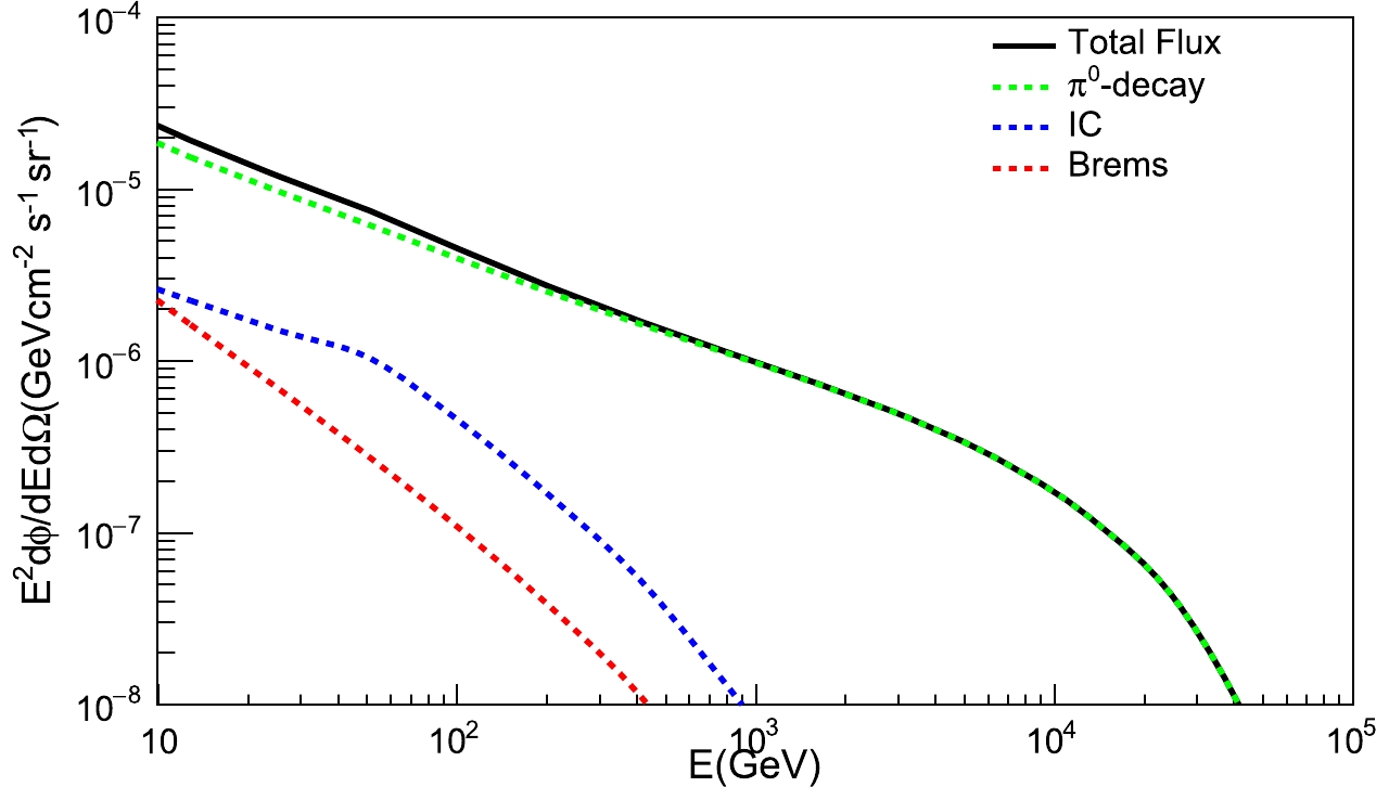
Figure 7. (color online) Average flux of the inner Galactic plane (
$22^\circ \leqslant l \leqslant 62^\circ, -2^\circ \leqslant b \leqslant 2^\circ$ , l is the Galactic longitude and b the Galactic latitude). The black line shows the total diffuse emission of the three processes, the dashed green line shows the$\gamma$ -rays produced in$\pi^{0}$ decays, the dashed blue and green lines denote the$\gamma$ -rays produced by electrons in the inverse Compton (IC) and bremsstrahlung processes.We generate two skymaps, one that considers only the TeV sources, and the other that shows only the diffuse emissions. The two skymaps are then combined to analyze the prospect of their detection with the one-year exposure. The one-dimensional projection of the significance is shown in Fig. 8. The red line is the standard normal distribution and the black line the significance distribution across the sky. For low values, the significance is well reproduced by the normal distribution. However, larger values are due to the
$ \gamma $ -ray sources and diffuse emission. The two-dimensional skymap is shown in Fig. 9. Although the significance of many of sources is greater than 15, the significance in Fig. 9 is limited to the range from -5 to 15 for visualization.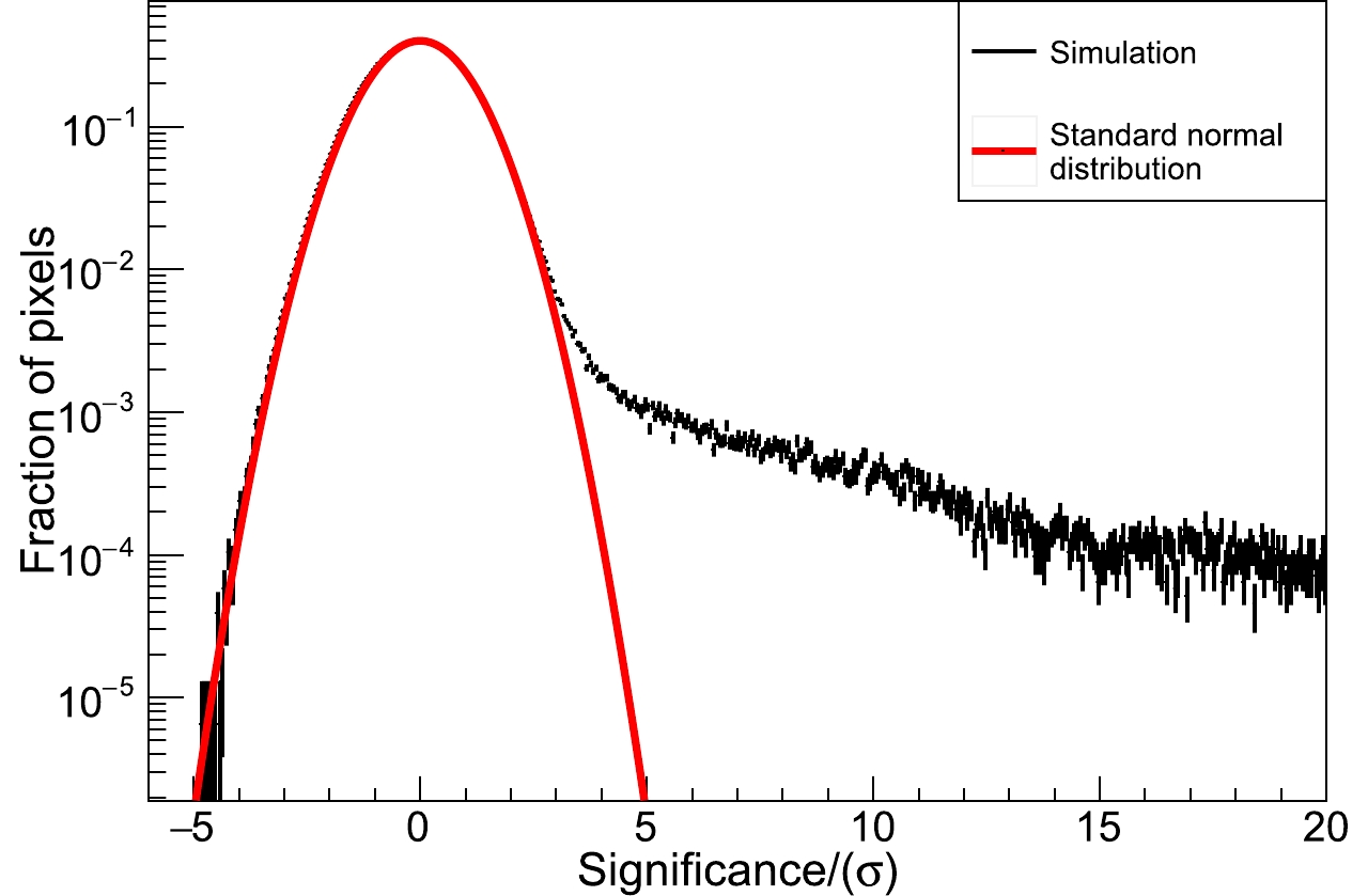
Figure 8. (color online) Significance distribution for the skymap (black line) and the standard normal distribution (red line).
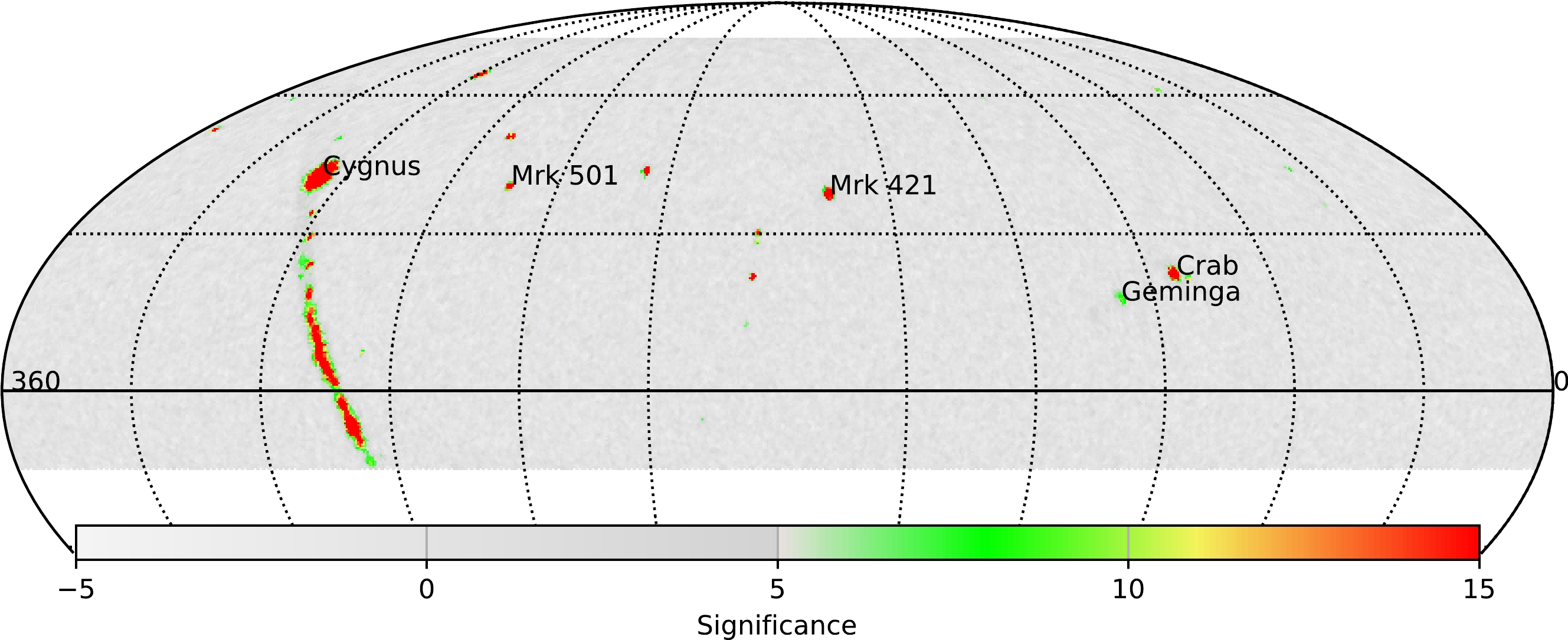
Figure 9. (color online) Significance of all TeV sources and diffuse emission in the equatorial coordinates (J2000.0 epoch). The significance is limited from -5 to 15 for visualization.
The combined skymap presented in Fig. 9 includes the TeV source signals and the diffuse emission. There are 22 sources (ARGO J2031+4157, LS I +61303, HESS J1912+101, W51, HESS J1831-098, 2HWC J1837-065, 2HWC J1825-134, MAGIC J1857.6+0297, TeV J1930+188, 2HWC J1844-032, 2HWC J1852+013, HESS J1858+020, 2HWC J2006+341, 2HWC J1902+048, 2HWC J1907+084, MGRO J1908+06, 2HWC J1914+117, 2HWC J1921+131,2HWC J1928+177, 2HWC J1938+238, 2HWC J1953+294, 2HWC J1955+285) in the Galactic plane (
$ -2^\circ \leqslant b \leqslant 2^\circ $ ), and the signals from these sources could be overestimated due to the diffuse$ \gamma $ -ray contributions in the combined skymap. We decompose the two components as described in Sec. 4 and calculate the signal count ($ N_{\rm calcu} $ ) from the combined map. To estimate the uncertainties due to the diffuse emission, we compare$ N_{\rm calcu} $ of the sources in the combined skymap with the signal count ($ N_{\rm detected} $ ) in the source map, since$ N_{\rm detected} $ is the source signal count considering that the source skymap excludes diffuse emission. The ratio of$ N_{\rm calcu} $ to$ N_{\rm detected} $ changes with$ N_{\rm detected} $ , as shown in Fig. 10.$ N_{\rm calcu} $ in the combined map tends to$ N_{\rm detected} $ for large source signal counts, and we can limit the uncertainty of the diffuse emission to the level of 20%, which agrees with the results in [11]. After subtracting the diffuse emission, the predicted significances and the information about the sources (location, spectrum, energy cutoff, extension) are presented in Tables 1,2,3,4. Among the sources with a significance greater than 5$ \sigma $ , there are 29 Galactic sources, constituting 20 unidentified sources, 4 PWN, and 5 other sources (superbubbles, SNRs, Shells and Binaries). There are 13 extragalactic sources, all of which are AGN. Another work [42] predicts that 9 sources (Mrk 421, 1ES 1215+303, 1ES 1218+304, W Comae, H 1426+428, 1ES 1959+650, Mrk 501, 1ES 2344+514, RGB J0710+591) could be detected after considering the extragalactic background light (EBL) absorption effect, which agrees with our results. We also predict that WCDA could detect M 87 with 6.82$ \sigma $ . This source is not included in Ref. [42]. Apart from these sources, the spectra of S3 0218+35 and RGB J2056+496 are measured in flare sates; the redshift of VER J0521+211 is more than 0.1, while we use an extrapolated spectrum from observation and do not consider the EBL absorption effect.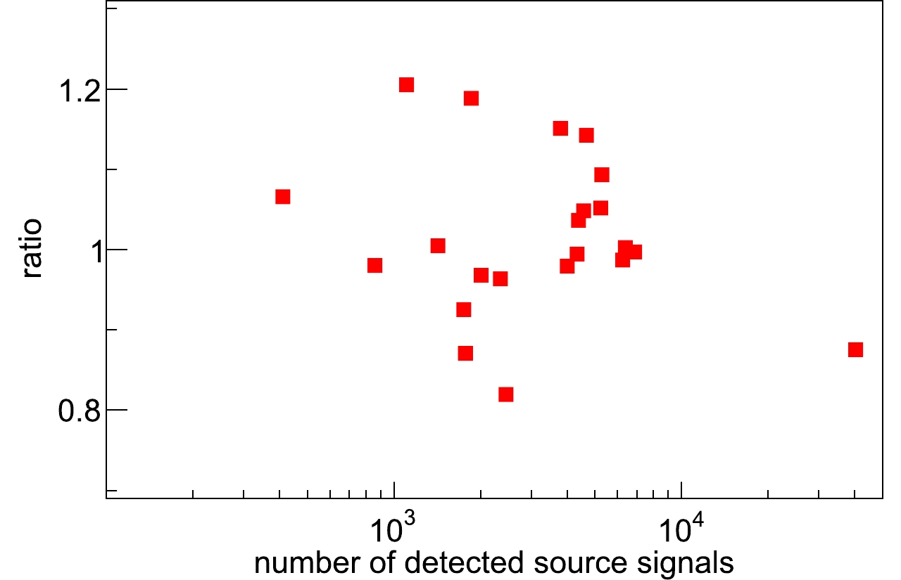
Figure 10. (color online) Uncertainty of the source signal count in the Galactic plane (
$-2^\circ \leqslant b \leqslant 2^\circ$ ) caused by the diffuse emission. The y-axis is the ratio of$N_{\rm calcu}$ to$N_{\rm detected}$ , and the x-axis is$N_{\rm detected}$ in the source skymap. -
WCDA is designed to detect
$ \gamma $ -rays from hundreds of GeV to tens of TeV for studies of the propagation and acceleration of cosmic rays. The results obtained in this work unveil the scientific potential of WCDA in the search for$ \gamma $ -ray sources. We study the$ \gamma $ -ray sources and the diffuse emissions simultaneously, and then determine the sources that have the potential to be observed with a significance of more than 5$ \sigma $ in a one-year exposure of WCDA.The ground-based IACTs have detected tens of AGN at VHE. Compared to IACTs, WCDA has a wide FOV and a long duty time, which increase its potential to detect AGN with long-term emissions. The prospects of WCDA to detect the already-known AGN are presented in Table 3. However, there are two uncertainties in these results. One is the unpredictable variability of the AGN flux. We use the measured time-averaged spectra rather than the spectra in flare states, and extend the spectra without energy cutoff. We also assume that these sources have constant flux, and then calculate the significance of their detection. The other uncertainty is due to the absorption effect by the extragalactic background light. We are limited to the nearby AGN (the redshift distances of these AGN are less than 0.13 except S3 0218+35) whose corresponding optical depth is less than 1, which means that the
$ \gamma $ -rays emitted by these AGN will not be strongly absorbed. Therefore, this work ignores the EBL absorption effect.As mentioned in Section 2, the design of WCDA has been modified. The new design is described in Ref. [ 14]. Its area is changed from 90,000
$ {\rm m}^2 $ to 78,000$ {\rm m}^2 $ since one large subarray measuring 300 m$ \times $ 110 m will replace two original subarrays. The number of detector units is 3,210,390, smaller than in the original design. A reduction in the effective area results in a sensitivity reduction of approximately 20%. Moreover, one detector unit consists of two PMTs at the center of each cell. In the first pond, each detector unit consists of one 8-inch and one 1.5-inch PMT, while each detector unit in the other two ponds consists of one 20-inch and one 3-inch PMT. The small PMTs are used for a joint observation with the Cherenkov telescope array (WFCTA) above 100 TeV, and the change from 8-inch PMTs to 20-inch PMTs aims to improve the sensitivity around 100 GeV. Since our analysis is performed at 1 TeV, these differences do not change our results significantly.
Prospects for a multi-TeV gamma-ray sky survey with the LHAASO water Cherenkov detector array
- Received Date: 2019-07-22
- Accepted Date: 2020-02-11
- Available Online: 2020-06-01
Abstract: The Water Cherenkov Detector Array (WCDA) is a major component of the Large High Altitude Air Shower Array Observatory (LHAASO), a new generation cosmic-ray experiment with unprecedented sensitivity, currently under construction. WCDA is aimed at the study of TeV


 DownLoad: