


 Abstract
 HTML
HTML Reference
 Related
 PDF
PDF


-
The LHCb collaboration in 2019 performed an angular analysis of weak decays
$ B^0\to J/\psi K^+\pi^- $ using proton-proton collision data, inspected$ m(J/\psi \pi^-) $ versus$ m(K^+\pi^-) $ planes, and observed two possible resonant structures in the vicinity of the energies$ m(J/\psi \pi^-) = $ $ 4200 \,\rm{MeV} $ and$ 4600\,\rm{MeV} $ , respectively [1]. There were two tentative proposals of the structure$ Z_c(4600) $ in the vicinity of$ m(J/\psi \pi^-) = 4600 \,\rm{MeV} $ , namely the$ [dc]_P[\bar{u}\bar{c}]_A-$ $ [dc]_A[\bar{u}\bar{c}]_P $ type vector tetraquark state with$ J^{PC} = 1^{--} $ [2] and the first radially excited$ [dc]_T[\bar{u}\bar{c}]_A-[dc]_A[\bar{u}\bar{c}]_T $ type tetraquark state with$ J^{PC} = 1^{+-} $ [3]. In this study, the subscripts P, S, V, A, and T represent the pseudoscalar, scalar, vector, axialvector, and tensor color-antitriplet diquark states, respectively.The BESIII collaboration in 2013 reported the charged charmonium-like resonance
$ Z^{\pm}_c(3900) $ in the$ \pi^\pm J/\psi $ invariant mass spectrum of the process$ e^+e^- \to J/\psi \pi^+\pi^- $ with$ M_{Z_c} = (3899.0\pm 3.6\pm 4.9)\,\rm{ MeV} $ and$ \Gamma_{Z_c} = (46\pm 10\pm 20) \,\rm{MeV} $ , respectively [4]. The Belle collaboration also observed$ Z^\pm_c(3900) $ in the same process [5]; furthermore, the CLEO collaboration confirmed the existence of the$ Z_c^\pm(3900) $ [6]. At around the same time, the BESIII collaboration observed the charmonium-like resonance$ Z^{\pm}_c(4025) $ in the vicinity of the threshold$ (D^{*} \bar{D}^{*})^{\pm} $ in the electron-positron scattering process$ e^+e^- \to (D^{*} \bar{D}^{*})^{\pm} \pi^\mp $ [7]. Moreover, the BESIII collaboration observed the charmonium-like resonance$ Z_c^\pm(4020) $ in the$ \pi^\pm h_c $ invariant mass spectrum of the electron-positron collisions$ e^+e^- \to \pi^+\pi^- h_c $ [8]. Presently,$ Z^\pm_c(4020) $ and$ Z^\pm_c(4025) $ are listed in The Review of Particle Physics as the same particle [9]. In 2014, the LHCb collaboration performed a four-dimensional fit of the scattering amplitude for the decay$ B^0\to\psi'\pi^-K^+ $ in proton-proton collisions and obtained the first independent confirmation of the charmonium-like resonance$ Z^-_c(4430) $ , determining its quantum numbers to be$ J^P = 1^+ $ [10]. In 2017, the BESIII collaboration established the quantum numbers of the charmonium-like resonance$ Z_c(3900) $ as$ J^P = 1^+ $ [11].There are several possible explanations for the exotic states
$ Z_c(3900) $ and$ Z_c(4020) $ , including the molecular states (from heavy quark symmetries [12, 13], QCD sum rules [14, 15], light-front quark model [16], one-pion exchange model [17], and phenomenological Lagrangian approach [18]), tetraquark states (from the diquark model with the effective Hamiltonian [19], QCD sum rules [20–23], and the potential model [24]), triangle singularities (in rescattering amplitudes) [25], threshold effects [26], etc.We can tentatively assign the hidden-charm resonances
$ Z_c(3900) $ and$ Z_c(4430) $ to the ground and first radially excited tetraquark state, respectively, considering their similar decays,$Z_c(3900)^\pm \to $ $ J/\psi\pi^\pm $ ,$Z_c(4430)^\pm \to $ $ \psi^\prime\pi^\pm $ , and the almost identical energy gaps$M_{Z_c(4430)}- $ $ M_{Z_c(3900)} = 591\,\rm{MeV} $ and$ M_{\psi^\prime}-M_{J/\psi} = 589 $ MeV [27, 28]. In Ref. [29], we adopted the method invented in Ref. [30] for the conventional quarkonium to study$ Z^\pm_c(3900) $ as the ground state axialvector tetraquark state and the$ Z^\pm_c(4430) $ as the first radially excited axialvector tetraquark state, respectively. We employed the energy scale formula$ \mu = \sqrt{M^2_{X/Y/Z}-(2{\mathbb{M}}_c)^2} $ to select optimal energy scales of spectral densities at the QCD side using the QCD sum rules method with the effective (or constituent) charm quark mass$ {\mathbb{M}}_c $ [31]. In Ref. [32], this subject is studied with the QCD sum rules by adopting another parameter system. In Refs. [22, 23],$ Z_c(4020/4025) $ can be assigned to be the ground state axialvector$ [uc]_A[\bar{d}\bar{c}]_A $ tetraquark state with the quantum numbers$ J^{PC} = 1^{+-} $ according to the QCD sum rules calculations. If$ Z_c(4600) $ is the first radial excitation of the hidden-charm tetraquark candidate$ Z_c(4020/4025) $ , its preferred decay mode is$Z_c(4600)\to $ $ \psi^\prime \pi $ , rather than$ Z_c(4600)\to J/\psi \pi $ .In this study, we perform a detailed and updated analysis of the ground and first radially excited states of the charged hidden-charm tetraquark states with QCD sum rules, and explore possible assignments of the
$ Z_c(4600) $ state in the scenario of the axialvector hidden-charm tetraquark states with the quantum numbers$ J^{PC} = 1^{+-} $ .This paper is structured as follows: in Sect. 2, we present the analytical expressions of the QCD sum rules obtained for the hidden-charm axialvector tetraquark states
$ Z_c $ . Sect. 3 provides numerical results for the masses and pole residues of$ Z_c $ states and presents further detailed discussions. The conclusions are provided in Sect. 4. -
In the following, we state the two-point Green functions (or correlation functions)
$ \Pi_{\mu\nu}(p) $ and$ \Pi_{\mu\nu\alpha\beta}(p) $ as the first step,$\begin{array}{l} {\Pi _{\mu \nu }}(p) = {\rm i}\displaystyle\int {{\rm d^4}} x{{\rm e}^{{\rm i}p \cdot x}}\langle 0|T\{ {J_\mu }(x)J_\nu ^\dagger (0)\} |0\rangle ,\\ {\Pi _{\mu \nu \alpha \beta }}(p) = {\rm i} \displaystyle\int {{\rm d^4}} x{{\rm e}^{{\rm i}p \cdot x}}\langle 0|T\{ {J_{\mu \nu }}(x)J_{\alpha \beta }^\dagger (0)\} |0\rangle , \end{array}$

(1) where the four-quark current operators
$ J_\mu(x) = J^1_\mu(x) $ ,$ J^2_\mu(x) $ ,$ J^3_\mu(x) $ ,$\begin{split} J_\mu ^1(x) =& \frac{{{\varepsilon ^{ijk}}{\varepsilon ^{imn}}}}{{\sqrt 2 }}[{u^{Tj}}(x)C{\gamma _5}{c^k}(x){{\bar d}^m}(x){\gamma _\mu }C{{\bar c}^{Tn}}(x) \\&- {u^{Tj}}(x)C{\gamma _\mu }{c^k}(x){{\bar d}^m}(x){\gamma _5}C{{\bar c}^{Tn}}(x)] ,\\ J_\mu ^2(x) =& \frac{{{\varepsilon ^{ijk}}{\varepsilon ^{imn}}}}{{\sqrt 2 }}[{u^{Tj}}(x)C{\sigma _{\mu \nu }}{\gamma _5}{c^k}(x){{\bar d}^m}(x){\gamma ^\nu }C{{\bar c}^{Tn}}(x) \\&- {u^{Tj}}(x)C{\gamma ^\nu }{c^k}(x){{\bar d}^m}(x){\gamma _5}{\sigma _{\mu \nu }}C{{\bar c}^{Tn}}(x)] , \end{split}$

$\begin{split} J_\mu ^3(x) =& \frac{{{\varepsilon ^{ijk}}{\varepsilon ^{imn}}}}{{\sqrt 2 }}[{u^{Tj}}(x)C{\sigma _{\mu \nu }}{c^k}(x){{\bar d}^m}(x){\gamma _5}{\gamma ^\nu }C{{\bar c}^{Tn}}(x) \\&+ {u^{Tj}}(x)C{\gamma ^\nu }{\gamma _5}{c^k}(x){{\bar d}^m}(x){\sigma _{\mu \nu }}C{{\bar c}^{Tn}}(x)] ,\\ {J_{\mu \nu }}(x) =& \frac{{{\varepsilon ^{ijk}}{\varepsilon ^{imn}}}}{{\sqrt 2 }}[{u^{Tj}}(x)C{\gamma _\mu }{c^k}(x){{\bar d}^m}(x){\gamma _\nu }C{{\bar c}^{Tn}}(x) \\&- {u^{Tj}}(x)C{\gamma _\nu }{c^k}(x){{\bar d}^m}(x){\gamma _\mu }C{{\bar c}^{Tn}}(x)] , \end{split}$

(2) the superscripts i, j, k, m, and n are color indexes with values obeying the antisymmetric tensor
$ \varepsilon $ and the charge conjugation matrix$ C = i\gamma^2\gamma^0 $ . If we preform the charge conjugation (and parity) transform$ \widehat{C} $ (and$ \widehat{P} $ ), the axialvector current operators$ J_\mu(x) $ and tensor current operator$ J_{\mu\nu}(x) $ have the following properties:$\begin{array}{ll} \hat C{J_\mu }(x){{\hat C}^{ - 1}} &= - {J_\mu }(x) ,\\ \hat C{J_{\mu \nu }}(x){{\hat C}^{ - 1}} &= - {J_{\mu \nu }}(x) ,\\ \hat P{J_\mu }(x){{\hat P}^{ - 1}} &= - {J^\mu }(\tilde x) ,\\ \hat P{J_{\mu \nu }}(x){{\hat P}^{ - 1}} &= {J^{\mu \nu }}(\tilde x) , \end{array}$

(3) where the coordinates
$ x^\mu = (t,\vec{x}) $ and$ \tilde{x}^\mu = (t,-\vec{x}) $ .The diquark operators
$ \varepsilon^{ijk}q^{T}_j C\Gamma Q_k $ in the attractive color-antitriplet$ \bar{3}_c $ channel have five spinor structures, where$ C\Gamma = C\gamma_5 $ , C,$ C\gamma_\mu \gamma_5 $ ,$ C\gamma_\mu $ , and$ C\sigma_{\mu\nu} $ or$ C\sigma_{\mu\nu}\gamma_5 $ correspond to the scalar, pseudoscalar, vector, axialvector, and tensor diquark operators, respectively. The favorable quark-quark correlations are the scalar diquark and axialvector diquark in the color-antitriplet$ \bar{3}_c $ channel from the QCD sum rules [33]. If we introduce a relative P-wave between the light quark and heavy quark, we can obtain the pseudoscalar diquark operator$ \varepsilon^{ijk}q^{T}_j C\gamma_5 \underline{\gamma_5}Q_k $ and vector diquark operator$ \varepsilon^{ijk}q^{T}_jC\gamma_\mu\underline{\gamma_5} Q_k $ without explicitly introducing the additional P-wave, as multiplying a$ \gamma_5 $ can change the parity, and the P-wave effect is embodied in the underlined$ \gamma_5 $ . Because the pseudoscalar and vector diquark states (or the P-wave diquark states) have larger masses compared to the scalar and axialvector diquark states, we choose the scalar diquark and axialvector diquark to construct the four-quark current operators to interpolate the lower tetraquark states.The tensor heavy diquark operators
$\varepsilon^{abc}q^{T}_b(x) $ $ C\sigma_{\mu\nu}\gamma_5Q_c(x) $ and$ \varepsilon^{abc}q^{T}_b(x)C\sigma_{\mu\nu}Q_c(x) $ have both axialvector and vector constituents,$\begin{split} &\hat P{\varepsilon ^{abc}}q_b^T(x)C{\sigma _{jk}}{\gamma _5}{Q_c}(x){{\hat P}^{ - 1}} = + {\varepsilon ^{abc}}q_b^T(\tilde x)C{\sigma _{jk}}{\gamma _5}{Q_c}(\tilde x) ,\\ &\hat P{\varepsilon ^{abc}}q_b^T(x)C{\sigma _{0j}}{Q_c}(x){{\hat P}^{ - 1}} = + {\varepsilon ^{abc}}q_b^T(\tilde x)C{\sigma _{0j}}{Q_c}(\tilde x) ,\\ &\hat P{\varepsilon ^{abc}}q_b^T(x)C{\sigma _{0j}}{\gamma _5}{Q_c}(x){{\hat P}^{ - 1}} = - {\varepsilon ^{abc}}q_b^T(\tilde x)C{\sigma _{0j}}{\gamma _5}{Q_c}(\tilde x) ,\\ &\hat P{\varepsilon ^{abc}}q_b^T(x)C{\sigma _{jk}}{Q_c}(x){{\hat P}^{ - 1}} = - {\varepsilon ^{abc}}q_b^T(\tilde x)C{\sigma _{jk}}{Q_c}(\tilde x) , \end{split}$

(4) where the space indexes j,
$ k = 1 $ , 2, 3. The tensor diquark operators also play an important role in constructing the tetraquark current operators [34]. We multiply the tensor diquark (antidiquark) operators with the axialvector or vector antidiquark (diquark) operators to project the axialvector and vector constituents and construct the four-quark current operators$ J^2_\mu(x) $ and$ J^3_\mu(x) $ . Thereafter, we use$ \tilde{V} $ and$ \tilde{A} $ to represent the vector and axialvector constituents of the tensor diquark operators, respectively.The four-quark current operators
$ J^1_\mu(x) $ ,$ J^2_\mu(x) $ , and$ J^3_\mu(x) $ potentially couple to the$ [uc]_S[\bar{d}\bar{c}]_A-[uc]_A[\bar{d}\bar{c}]_S $ type,$ [uc]_{\tilde{A}}[\bar{d}\bar{c}]_A-[uc]_A[\bar{d}\bar{c}]_{\tilde{A}} $ type, and$ [uc]_{\tilde{V}}[\bar{d}\bar{c}]_V +$ $ [uc]_V[\bar{d}\bar{c}]_{\tilde{V}} $ type axialvector hidden-charm tetraquark states with the spin-parity-charge-conjugation$ J^{PC} = 1^{+-} $ , respectively. Meanwhile, the current operator$ J_{\mu\nu}(x) $ potentially couples to both the$ [uc]_A[\bar{d}\bar{c}]_A $ type axialvector tetraquark state with$ J^{PC} = 1^{+-} $ and the vector tetraquark state with$ J^{PC} = 1^{--} $ . Hereafter, we do not distinguish the negative or positive electric-charge of$ Z_c $ tetraquark states, as they have degenerate masses.We insert a complete set of hadron states that have nonvanishing couplings with the four-quark current operators
$ J_\mu(x) $ and$ J_{\mu\nu}(x) $ into the Green functions$ \Pi_{\mu\nu}(p) $ and$ \Pi_{\mu\nu\alpha\beta}(p) $ to obtain the hadronic representation [35, 36]. Then, we separate the ground state axialvector and vector tetraquark state contributions from other contributions, such as the higher excited tetraquark and continuum states, to obtain the results,$\begin{split} {\Pi _{\mu \nu }}(p) =& \frac{{\lambda _Z^2}}{{m_Z^2 - {p^2}}}\left( { - {g_{\mu \nu }} + \frac{{{p_\mu }{p_\nu }}}{{{p^2}}}} \right) + \cdots \\ =& {\Pi _Z}({p^2})\left( { - {g_{\mu \nu }} + \frac{{{p_\mu }{p_\nu }}}{{{p^2}}}} \right) + \cdots , \end{split}$

(5) $\begin{split} {\Pi _{\mu \nu \alpha \beta }}(p) =& \frac{{\tilde \lambda _Z^2}}{{m_Z^2 - {p^2}}}\left( {{p^2}{g_{\mu \alpha }}{g_{\nu \beta }} - {p^2}{g_{\mu \beta }}{g_{\nu \alpha }} - {g_{\mu \alpha }}{p_\nu }{p_\beta } - {g_{\nu \beta }}{p_\mu }{p_\alpha } + {g_{\mu \beta }}{p_\nu }{p_\alpha } + {g_{\nu \alpha }}{p_\mu }{p_\beta }} \right)\\ & + \frac{{\tilde \lambda _Y^2}}{{m_Y^2 - {p^2}}}\left( { - {g_{\mu \alpha }}{p_\nu }{p_\beta } - {g_{\nu \beta }}{p_\mu }{p_\alpha } + {g_{\mu \beta }}{p_\nu }{p_\alpha } + {g_{\nu \alpha }}{p_\mu }{p_\beta }} \right) + \cdots \\ =& {\Pi _Z}({p^2})\left( {{p^2}{g_{\mu \alpha }}{g_{\nu \beta }} - {p^2}{g_{\mu \beta }}{g_{\nu \alpha }} - {g_{\mu \alpha }}{p_\nu }{p_\beta } - {g_{\nu \beta }}{p_\mu }{p_\alpha } + {g_{\mu \beta }}{p_\nu }{p_\alpha } + {g_{\nu \alpha }}{p_\mu }{p_\beta }} \right)\\ &+ {\Pi _Y}({p^2})\left( { - {g_{\mu \alpha }}{p_\nu }{p_\beta } - {g_{\nu \beta }}{p_\mu }{p_\alpha } + {g_{\mu \beta }}{p_\nu }{p_\alpha } + {g_{\nu \alpha }}{p_\mu }{p_\beta }} \right) , \end{split}$

(6) where Z represents the axialvector tetraquark states; Y represents the vector tetraquark states;
$ \lambda_{Z} $ ,$ \widetilde{\lambda}_{Z} $ and$ \widetilde{\lambda}_{Y} $ are the pole residues or current-tetraquark coupling constants,$\begin{split} \langle 0|{J_\mu }(0)|{Z_c}(p)\rangle = &{\lambda _Z} {\varepsilon _\mu } ,\\ \langle 0|{J_{\mu \nu }}(0)|{Z_c}(p)\rangle =& {{\tilde \lambda }_Z} {\varepsilon _{\mu \nu \alpha \beta }} {\varepsilon ^\alpha }{p^\beta } ,\\ \langle 0|{J_{\mu \nu }}(0)|Y(p)\rangle = &{{\tilde \lambda }_Y}\left( {{\varepsilon _\mu }{p_\nu } - {\varepsilon _\nu }{p_\mu }} \right) , \end{split}$

(7) where the antisymmetric tensor
$ \varepsilon_{0123} = -1 $ , and$ \varepsilon_\mu(\lambda,p) $ depicts polarization vectors of the axialvector and vector tetraquark states, which satisfy the summation formula,$\sum\limits_\lambda {\varepsilon _\mu ^*} (\lambda ,p){\varepsilon _\nu }(\lambda ,p) = - {g_{\mu \nu }} + \frac{{{p_\mu }{p_\nu }}}{{{p^2}}} .$

(8) The diquark-antidiquark type four-quark current operators
$ J_\mu(x) $ and$ J_{\mu\nu}(x) $ potentially couple to the diquark-antidiquark type hidden-charm tetraquark states. We perform Fierz rearrangements to those currents in both the spinor space and color space to obtain a series of color-singlet-color-singlet (or meson-meson) type current operators, for example,$\begin{split} J_\mu ^1(x) =& \frac{1}{{2\sqrt 2 }}\{ i\bar c(x)i{\gamma _5}c(x) \bar d(x){\gamma ^\mu }u(x) - i\bar c(x){\gamma ^\mu }c(x) \bar d(x)i{\gamma _5}u(x) + \bar c(x)u(x) \bar d(x){\gamma ^\mu }{\gamma _5}c(x)\\ &- \bar c(x){\gamma ^\mu }{\gamma _5}u(x) \bar d(x)c(x) - i\bar c(x){\gamma _\nu }{\gamma _5}c(x) \bar d(x){\sigma ^{\mu \nu }}u(x) + i\bar c(x){\sigma ^{\mu \nu }}c(x) \bar d(x){\gamma _\nu }{\gamma _5}u(x)\\ & - i\bar c(x){\sigma ^{\mu \nu }}{\gamma _5}u(x) \bar d(x){\gamma _\nu }c(x) + i\bar c(x){\gamma _\nu }u(x) \bar d(x){\sigma ^{\mu \nu }}{\gamma _5}c(x) \} , \end{split}$

(9) while the constituents, like
$ \bar{c}(x)i\gamma_5 c(x)\,\bar{d}(x)\gamma^\mu u(x) $ ,$ \bar{c}(x) \gamma^\mu c(x)\,\bar{d}(x)i\gamma_5 u(x) $ , etc, potentially couple to the meson-meson type scattering or tetraquark molecular states.However, we must be careful in performing the Fierz rearrangements, where the rearrangements in the spinor space and color space are quite non-trivial, and the scenarios of the diquark-antidiquark type tetraquark states and meson-meson type molecular states are considerably different.
According to the arguments by Selem and Wilczek, a diquark-antidiquark type tetraquark may be described by two diquarks trapped in a double potential well, where the two potential wells are separated apart by a barrier [37]. At long distances, the diquark and antiquark serve as point color charges and attract each other strongly, just like in the quark and antiquark bound states. However, when the two diquarks approach each other, the attractions between the quark and antiquark in different diquarks decrease the bonding energy of the diquarks and tend to destroy the diquarks. Those effects (beyond the naive one-gluon exchange force) increase when the distance between the diquark and antidiquark decreases, and a repulsive interaction between the diquark and antidiquark emerges. If this repulsion is large enough, it leads to a barrier between the diquark and antidiquark [38]. The two potential wells that are separated by a barrier can provide good descriptions of the diquark-antidiquark type tetraquark states [38].
Meanwhile, in the dynamical picture of the tetraquark states, the large spatial separation between the diquark and antidiquark leads to a small wave-function overlap between the quark-antiquark pair [39], and the rearrangements in the spinor space and color space are highly suppressed.
It is difficult to account for the non-local effects between the diquark and antidiquark pair in the four-quark currents
$ J_\mu(x) $ and$ J_{\mu\nu}(x) $ directly in practical calculations. For example, the current$ J^1_\mu(x) $ can be modified to$\begin{split} J_\mu ^1(x,\epsilon ) =& \frac{{{\varepsilon ^{ijk}}{\varepsilon ^{imn}}}}{{\sqrt 2 }}[{u^{Tj}}(x)C{\gamma _5}{c^k}(x){{\bar d}^m}(x + \epsilon ){\gamma _\mu }C{{\bar c}^{Tn}}(x + \epsilon ) \\&- {u^{Tj}}(x)C{\gamma _\mu }{c^k}(x){{\bar d}^m}(x + \epsilon ){\gamma _5}C{{\bar c}^{Tn}}(x + \epsilon )] , \end{split}$

(10) to account for the non-locality by adding a finite
$ \epsilon $ ; however, it is highly difficult to deal with the finite$ \epsilon $ both at the hadron side and at the QCD side in a consistent manner. Hence, we express the current$ J^1_\mu(x,\epsilon) $ in terms of the Taylor series of$ \epsilon $ ,$J_\mu ^1(x,\epsilon ) = J_\mu ^1(x,0) + \frac{{\partial J_\mu ^1(x,\epsilon )}}{{\partial {\epsilon ^\alpha }}}{\bigg| _{\epsilon = 0}}{\epsilon ^\alpha } + \frac{1}{2}\frac{{{\partial ^2}J_\mu ^1(x,\epsilon )}}{{\partial {\epsilon ^\alpha }\partial {\epsilon ^\beta }}}{\bigg| _{\epsilon = 0}}{\epsilon ^\alpha }{\epsilon ^\beta } + \cdots ,$

(11) then we express the correlation function
$ \Pi_{\mu\nu}(p) $ likewise in terms of the Taylor series of$ \epsilon $ ,${\Pi _{\mu \nu }}(p) = {\Pi _{\mu \nu }}\left( {{\cal O}({\epsilon ^0})} \right) + {\Pi _{\mu \nu }}\left( {{\cal O}({\epsilon ^1})} \right) + {\Pi _{\mu \nu }}\left( {{\cal O}({\epsilon ^2})} \right) + \cdots ,$

(12) where the components
$ \Pi_{\mu\nu}\left({\cal O}(\epsilon^i)\right) $ with$ i = 0 $ , 1, 2,$ \cdots $ represent the contributions of the order$ {\cal O}(\epsilon^i) $ . In this article, we study the leading order contributions$J^1_\mu(x) = $ $ J^1_\mu(x,0) $ and$ \Pi_{\mu\nu}(p) = \Pi_{\mu\nu}\left({\cal O}(\epsilon^0)\right) $ . The effects beyond the leading order frustrate the Fierz rearrangements of the diquark-antidiquark type currents into a series of color-singlet-color-singlet (meson-meson) type currents freely.We employ the Feynman diagram drawn in Fig. 1 to describe the lowest order contributions in the correlation functions for the diquark-antidiquark type four-quark currents and use the Feynman diagrams drawn in Fig. 2 to describe the corresponding lowest order contributions in the correlation functions for the color-singlet-color-singlet type four-quark currents. The Feynman diagram drawn in Fig. 1 cannot be freely factorized into the two Feynman diagrams drawn in Fig. 2 due to the barrier (or spatial separation) between the diquark and antidiquark [38, 39]. When a quark (antiquark) in the diquark (antidiquark) penetrates the barrier, the Feynman diagram drawn in Fig. 1 is factorizable in color space. In this case, the non-factorizable diagrams start at the order
$ {\cal O}(\alpha_s^2) $ [40].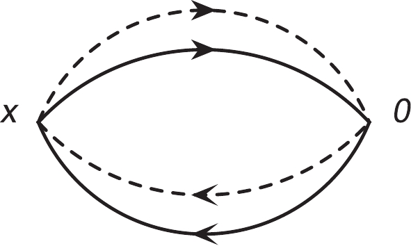
Figure 1. Feynman diagram of lowest order contributions for diquark-antidiquark type currents, where solid lines represent light quarks, and dashed lines represent heavy quarks.
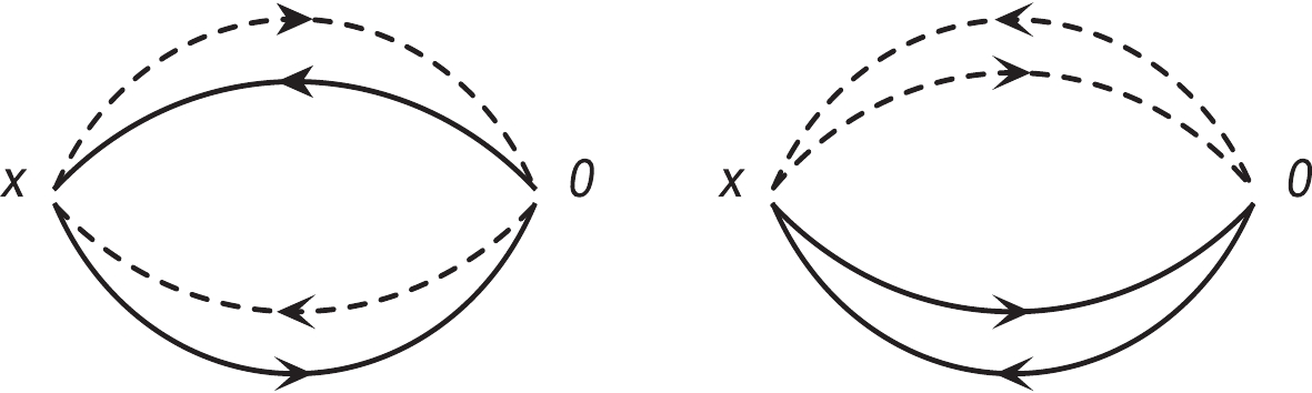
Figure 2. Feynman diagrams of lowest order contributions for color-singlet-color-singlet type currents, where solid lines represent light quarks and dashed lines represent heavy quarks.
In Ref. [40], Lucha, Melikhov, and Sazdjiand argued that the diquark-antidiquark type four-quark currents can be changed into color-singlet-color-singlet (meson-meson) type currents through the Fierz transformation. The Feynman diagrams, which make contributions to the quark-gluon operators of the order
$ {\cal O}(\alpha_s^0) $ and$ {\cal O}(\alpha_s) $ in accomplishing the operator product expansion are factorizable, and they are canceled out by the contributions of the two-meson scattering states at the phenomenological side. Furthermore, the factorizable parts (in color space) of the Feynman diagrams of the order$ {\cal O}(\alpha_s^2) $ are also canceled out by contributions from the two-meson scattering states (or more precisely, the free two-meson states). The relevant non-factorizable contributions start at the order$ {\cal O}(\alpha_s^2) $ . We do not agree with their viewpoint, as there is a repulsive barrier [37, 38] or a large spatial separation [39] embodied in the non-local effects to prevent freely performing the Fierz transformation, although at the present time we cannot take into account non-local effects in the QCD sum rules and have to assume the leading order approximations$ J^1_\mu(x) = J^1_\mu(x,0) $ and$ \Pi_{\mu\nu}(p) = \Pi_{\mu\nu}\left({\cal O}(\epsilon^0)\right) $ . Our viewpoint is that the relevant contributions begin at the order$ {\cal O}(\alpha_s^0) $ , and it is not necessary or it is very difficult to perform the Fierz transformation to separate factorizable and non-factorizable contributions in the color space. Hence, we should take into account both the factorizable and nonfactorizable Feynman diagrams for the diquark-antidiquark type currents.When the quark or antiquark penetrates the barrier, we can perform the Fierz rearrangements and study the effects of the scattering states. Thus, we explore the contributions of the meson-meson type scattering states (in other words, the two-meson loops) to the Green function
$ \Pi_{\mu\nu}(p) $ for the four-quark current$ J^1_\mu(x) $ as a representative example,$\begin{split} {\Pi _{\mu \nu }}(p) =& - \frac{{\widehat \lambda _Z^2}}{{{p^2} - \widehat M_Z^2}}{{\tilde g}_{\mu \nu }}(p) - \frac{{{{\widehat \lambda }_Z}}}{{{p^2} - \widehat M_Z^2}}{{\tilde g}_{\mu \alpha }}(p){\Sigma _{D{D^*}}}(p){{\tilde g}^{\alpha \beta }}(p){{\tilde g}_{\beta \nu }}(p)\frac{{{{\widehat \lambda }_Z}}}{{{p^2} - \widehat M_Z^2}}\\ & - \frac{{{{\widehat \lambda }_Z}}}{{{p^2} - \widehat M_Z^2}}{{\tilde g}_{\mu \alpha }}(p){\Sigma _{J/\psi \pi }}(p){{\tilde g}^{\alpha \beta }}(p){{\tilde g}_{\beta \nu }}(p)\frac{{{{\widehat \lambda }_{X/Z}}}}{{{p^2} - \widehat M_Z^2}} + \cdots ,\\ =& - \frac{{\widehat \lambda _Z^2}}{{{p^2} - \widehat M_Z^2 - {\Sigma _{D{D^*}}}(p) - {\Sigma _{J/\psi \pi }}(p) + \cdots }}{{\tilde g}_{\mu \nu }}(p) + \cdots , \end{split}$

(13) where
$\begin{split} {\Sigma _{D{D^*}}}(p) =& {\rm i}\int \; \frac{{{\rm d^4}q}}{{{{(2\pi )}^4}}}\frac{{G_{ZD{D^*}}^2}}{{\left[ {{q^2} - M_D^2} \right]\left[ {{{(p - q)}^2} - M_{{D^*}}^2} \right]}} ,\\ {\Sigma _{J/\psi \pi }}(p) =& {\rm i}\int \; \frac{{{\rm d^4}q}}{{{{(2\pi )}^4}}}\frac{{G_{ZJ/\psi \pi }^2}}{{\left[ {{q^2} - M_{J/\psi }^2} \right]\left[ {{{(p - q)}^2} - M_\pi ^2} \right]}} , \end{split}$

(14) $ \widetilde{g}_{\mu\nu}(p) = -g_{\mu\nu}+\frac{p_{\mu}p_{\nu}}{p^2} $ , and the$ G_{Z DD^*} $ and$ G_{Z J/\psi\pi} $ are the hadronic coupling constants. We resort to the bare quantities$ \widehat{\lambda}_{Z} $ and$ \widehat{M}_{Z} $ so as to absorb the divergent terms that appear in the integrals in calculating the self-energies$ \Sigma_{DD^*}(p) $ ,$ \Sigma_{J/\psi \pi}(p) $ , etc. The self-energies after renormalization result in a finite energy-dependent width to modify the dispersion relation,${\Pi _{\mu \nu }}(p) = - \frac{{\lambda _Z^2}}{{{p^2} - M_Z^2 + {\rm i}\sqrt {{p^2}} \Gamma ({p^2})}}{\tilde g_{\mu \nu }}(p) + \cdots ,$

(15) where the experimental value of the total decay width
$ \Gamma_{Z_c(3900)}(M_Z^2) = (46\pm 10\pm 20) \,\rm{MeV} $ [4] (or$ (28.2\pm 2.6)\, \rm{MeV} $ [9]), and the zero width approximation of spectral densities at the phenomenological side are considered reasonable [41]. In this study, we neglect contributions of the meson-meson type scattering states or the two-meson loops, and the predictions remain robust.We calculate all Feynman diagrams in performing the operator product expansion to obtain the QCD spectral representation of the Green functions (or correlation functions)
$ \Pi_{\mu\nu}(p) $ and$ \Pi_{\mu\nu\alpha\beta}(p) $ . In the analytical calculations, we consistently take into account vacuum condensates (by selecting the quark-gluon operators of the orders$ {\cal O}( \alpha_s^{k}) $ with$ k\leq 1 $ ) up to dimension$ 10 $ and factorize higher dimensional condensates into lower dimensional condensates by assuming vacuum saturation. After obtaining the analytical expressions of the Green functions at the quark-gluon level, we obtain the spectral representation via the dispersion relation. Then, we match the hadronic representation with the QCD representation of the Green functions (or correlation functions)$ \Pi_Z(p^2) $ below the continuum threshold parameters$ s_0 $ and carry out the Borel transformation with regard to$ P^2 = -p^2 $ to obtain the QCD sum rules:$\lambda _Z^2 \exp \left( { - \frac{{M_Z^2}}{{{T^2}}}} \right) = \int_{4m_c^2}^{{s_0}} {\rm d} s \rho (s) \exp \left( { - \frac{s}{{{T^2}}}} \right) ,$

(16) $\begin{split}\rho (s) =& {\rho _0}(s) + {\rho _3}(s) + {\rho _4}(s) + {\rho _5}(s) + {\rho _6}(s) \\&+ {\rho _7}(s) + {\rho _8}(s) + {\rho _{10}}(s) ,\end{split}$

(17) $ \lambda_Z = \widetilde{\lambda}_Z M_Z $ , the$ T^2 $ is the Borel parameter, the subscript i in the components of the QCD spectral densities$ \rho_{i}(s) $ represents the dimensions of the vacuum condensates,$\begin{split} {\rho _3}(s) \propto & \langle \bar qq\rangle ,\\ {\rho _4}(s) \propto & \langle \frac{{{\alpha _s}GG}}{\pi }\rangle ,\\ {\rho _5}(s) \propto & \langle \bar q{g_s}\sigma Gq\rangle ,\\ {\rho _6}(s) \propto & {\langle \bar qq\rangle ^2} , 4\pi {\alpha _s}{\langle \bar qq\rangle ^2} ,\\ {\rho _7}(s) \propto & \langle \bar qq\rangle \langle \frac{{{\alpha _s}GG}}{\pi }\rangle ,\\ {\rho _8}(s) \propto & \langle \bar qq\rangle \langle \bar q{g_s}\sigma Gq\rangle ,\\ {\rho _{10}}(s) \propto & {\langle \bar q{g_s}\sigma Gq\rangle ^2} , {\langle \bar qq\rangle ^2}\langle \frac{{{\alpha _s}GG}}{\pi }\rangle . \end{split}$

(18) We neglect the cumbersome analytical expressions of spectral densities at the quark-gluon level in saving printed pages. We refer to Ref. [20] for technical details on calculating the Feynman diagrams. In contrast, we refer to Refs. [20, 23] for explicit expressions of spectral densities at the quark-gluon level for the axialvector current
$ J^1_\mu(x) $ and tensor current$ J_{\mu\nu}(x) $ . In this study, we recalculate those QCD spectral densities, and use the formula$ t^a_{ij}t^a_{mn} = -\dfrac{1}{6}\delta_{ij}\delta_{mn}+\dfrac{1}{2}\delta_{jm}\delta_{in} $ with$ t^a = \dfrac{\lambda^a}{2} $ to deal with the higher dimensional vacuum condensates, where$ \lambda^a $ is the Gell-Mann matrix. This routine leads to slight but neglectful differences compared to old calculations. For the currents$ J^2_\mu(x) $ and$ J^3_\mu(x) $ , we neglect the tiny contributions of$ 4\pi\alpha_s\langle\bar{q}q\rangle^2 $ , which originate from operators such as$ \langle\bar{q}_j\gamma_{\mu}q_ig_s D_\nu G^a_{\alpha\beta}t^a_{mn}\rangle $ .We derive Eq. (16) with regard to
$ \tau = \dfrac{1}{T^2} $ , then reach the QCD sum rules for the tetraquark masses by eliminating the pole residues$ \lambda_{Z} $ through a fraction,$M_Z^2 = - \frac{{\displaystyle\int_{4m_c^2}^{{s_0}} {\rm d} s \dfrac{\rm d}{{\rm d\tau }} \rho (s){{\rm e}^{ - \tau s}}}}{{\displaystyle\int_{4m_c^2}^{{s_0}} {\rm d} s\rho (s){{\rm e}^{ - \tau s}}}} .$

(19) Thereafter, we refer the QCD sum rules in Eq. (16) and Eq. (19) as QCDSR I.
If we take into account the contributions of the first radially excited tetraquark states
$ Z_c^\prime $ in the hadronic representation, we obtain the QCD sum rules,$\lambda _Z^2 \exp \left( { - \frac{{M_Z^2}}{{{T^2}}}} \right) + \lambda _{{Z^\prime }}^2 \exp \left( { - \frac{{M_{{Z^\prime }}^2}}{{{T^2}}}} \right) = \int_{4m_c^2}^{s_0^\prime } {\rm d} s \rho (s) \exp \left( { - \frac{s}{{{T^2}}}} \right) ,$

(20) where
$ s_0^\prime $ is the continuum threshold parameter. Subsequently, we introduce the notations$ \tau = \dfrac{1}{T^2} $ ,$ D^n = \left( -\dfrac{\rm d}{\rm d\tau}\right)^n $ , and resort to the subscripts 1 and 2 to represent the ground state tetraquark state$ Z_c $ and the first radially excited tetraquark state$ Z_c^\prime $ for simplicity. We rewrite the QCD sum rules as$\lambda _1^2\exp \left( { - \tau M_1^2} \right) + \lambda _2^2\exp \left( { - \tau M_2^2} \right) = {\Pi _{\rm QCD}}(\tau ) ,$

(21) where we introduce the subscript
$ {\rm QCD} $ to denote the QCD representation. We derive the QCD sum rules in Eq. (21) with respect to$ \tau $ to get$\lambda _1^2M_1^2\exp \left( { - \tau M_1^2} \right) + \lambda _2^2M_2^2\exp \left( { - \tau M_2^2} \right) = D{\Pi _{\rm QCD}}(\tau ) .$

(22) From Eqs. (21)–(22), we obtain the QCD sum rules,
$\lambda _i^2\exp \left( { - \tau M_i^2} \right) = \frac{{\left( {D - M_j^2} \right){\Pi _{\rm QCD}}(\tau )}}{{M_i^2 - M_j^2}} ,$

(23) where the indexes
$ i \neq j $ . We derive the QCD sum rules in Eq. (23) with respect to$ \tau $ to get$\begin{split} M_i^2 = \frac{{\left( {{D^2} - M_j^2D} \right){\Pi _{\rm QCD}}(\tau )}}{{\left( {D - M_j^2} \right){\Pi _{\rm QCD}}(\tau )}} ,\quad M_i^4 = \frac{{\left( {{D^3} - M_j^2{D^2}} \right){\Pi _{\rm QCD}}(\tau )}}{{\left( {D - M_j^2} \right){\Pi _{\rm QCD}}(\tau )}} . \end{split}$

(24) The squared masses
$ M_i^2 $ satisfy the equation,$M_i^4 - bM_i^2 + c = 0 ,$

(25) where
$\begin{split} b = &\frac{{{D^3} \otimes {D^0} - {D^2} \otimes D}}{{{D^2} \otimes {D^0} - D \otimes D}} ,\\ c =& \frac{{{D^3} \otimes D - {D^2} \otimes {D^2}}}{{{D^2} \otimes {D^0} - D \otimes D}} ,\\ {D^j} \otimes {D^k} = &{D^j}{\Pi _{\rm QCD}}(\tau ) {D^k}{\Pi _{\rm QCD}}(\tau ) , \end{split}$

(26) where the indexes
$ i = 1,2 $ and$ j,k = 0,1,2,3 $ . Finally, we solve above equation analytically to obtain two solutions [30],$M_1^2 = \frac{{b - \sqrt {{b^2} - 4c} }}{2} ,$

(27) $M_2^2 = \frac{{b + \sqrt {{b^2} - 4c} }}{2} .$

(28) From hereon forward, we denote the QCD sum rules in Eq. (20) and Eqs. (27)–(28) as QCDSR II. In calculations, we observe that if we specify the energy scales of the spectral densities in the QCD representation, only one solution satisfies the energy scale formula
$ \mu = \sqrt{M^2_{X/Y/Z}-(2{\mathbb{M}}_c)^2} $ in the QCDSR II, and we have to abandon the other solution. In this study, we retain the mass$ M_2 $ ($ M_{Z^\prime} $ ) and discard the mass$ M_1 $ ($ M_Z $ ). -
We assume the standard values or conventional values of the vacuum condensates
$ \langle\bar{q}q \rangle = -(0.24\pm 0.01\, \rm{GeV})^3 $ ,$ \langle\bar{q}g_s\sigma G q \rangle \!\!=\!\! m_0^2\langle \bar{q}q \rangle $ ,$ m_0^2 \!=\! (0.8 \!\pm \!0.1)\,\rm{GeV}^2 $ ,$ \langle \frac{\alpha_s GG}{\pi}\rangle \!\!=\!\! (0.33\,\rm{GeV})^4 $ at the typical energy scale$ \mu = 1\, \rm{GeV} $ [35, 36, 42], and take the modified minimal subtraction mass of the charm quark$ m_{c}(m_c) = (1.275\pm0.025)\,\rm{GeV} $ from the Particle Data Group [9]. We must evolve the quark condensate, mixed quark condensate, and modified minimal subtraction mass to a special energy scale to warrant the parameters in QCD spectral densities with the same energy scale. Then, we account for the energy-scale dependence of the input parameters at the quark-gluon level,$\begin{split} \langle \bar qq\rangle (\mu ) =& \langle \bar qq\rangle ({\rm{1GeV}}){\left[ {\frac{{{\alpha _s}({\rm{1GeV}})}}{{{\alpha _s}(\mu )}}} \right]^{\frac{{12}}{{33 - 2{n_f}}}}} ,\\ \langle \bar q{g_s}\sigma Gq\rangle (\mu ) =& \langle \bar q{g_s}\sigma Gq\rangle ({\rm{1GeV}}){\left[ {\frac{{{\alpha _s}({\rm{1GeV}})}}{{{\alpha _s}(\mu )}}} \right]^{\frac{2}{{33 - 2{n_f}}}}} ,\\ {m_c}(\mu ) =& {m_c}({m_c}){\left[ {\frac{{{\alpha _s}(\mu )}}{{{\alpha _s}({m_c})}}} \right]^{\frac{{12}}{{33 - 2{n_f}}}}} ,\\ {\alpha _s}(\mu ) =& \frac{1}{{{b_0}t}}\left[ {1 - \frac{{{b_1}}}{{b_0^2}}\frac{{\log t}}{t} + \frac{{b_1^2({{\log }^2}t - \log t - 1) + {b_0}{b_2}}}{{b_0^4{t^2}}}} \right] , \end{split}$

(29) where
$ t = \log \dfrac{\mu^2}{\Lambda^2} $ ,$ b_0 = \dfrac{33-2n_f}{12\pi} $ ,$ b_1 = \dfrac{153-19n_f}{24\pi^2} $ ,$ b_2 = \dfrac{2857-\frac{5033}{9}n_f+\frac{325}{27}n_f^2}{128\pi^3} $ , with the values$ \Lambda = 210\,\rm{MeV} $ ,$ 292\,\rm{MeV} $ , and$ 332\,\rm{MeV} $ for the quark flavors$ n_f = 5 $ , 4, and 3, respectively [9, 43]. As we explore the hidden-charm tetraquark states, we choose the flavor$ n_f = 4 $ and search for the best energy scales$ \mu $ .The Okubo-Zweig-Iizuka super-allowed decays
$\begin{array}{l} {Z_c} \to J/\psi \pi ,\ \ Z_c^\prime \to {\psi ^\prime }\pi , \ \ Z_c^{\prime \prime } \to {\psi ^{\prime \prime }}\pi , \end{array}$

(30) are expected to easily take place. The energy gaps maybe have the relations
$ M_{Z^\prime}-M_{Z} = m_{\psi^\prime}-m_{J/\psi} $ and$M_{Z^{\prime\prime}}-M_{Z^\prime} = $ $ m_{\psi^{\prime\prime}}-m_{\psi^\prime} $ . The charmonium masses are$ m_{J/\psi} = 3.0969$ GeV,$ m_{\psi^\prime} = 3.686097 $ GeV, and$ m_{\psi^{\prime\prime}} = 4.039 $ GeV from the Particle Data Group [9],$ m_{\psi^\prime}-m_{J/\psi} = 0.59 $ GeV,$ m_{\psi^{\prime\prime}}-m_{J/\psi} = $ 0.94 GeV. We choose the continuum threshold parameters to be$ \sqrt{s_0} = M_{Z}+0.59\,\rm{GeV} $ and$ \sqrt{s_0^\prime} = M_{Z}+ $ 0.95 GeV tentatively and vary the continuum threshold and Borel parameters to satisfy the following four criteria:1. The ground state tetraquark state or single-pole term makes the dominant contribution at the hadron side;
2. The operator product expansion is convergent below continuum thresholds, and the higher dimensional vacuum condensates make a minor contribution;
3. The Borel platforms appear in both the lineshapes of the tetraquark masses and pole residues with variations of the Borel parameters;
4. The masses of the tetraquark states satisfy the energy-scale formula.
After trial and error, we reach the feasible continuum threshold parameters and Borel windows. We also acquire the optimal energy scales of the spectral densities at the quark-gluon level and the contributions of the ground state tetraquark states for the QCDSR I, as shown in Table 1. In general, for the continuum threshold parameters
$ s_0 $ , we can assume that any values satisfy the relation$ M_{gr}<\sqrt{s_0}\leqslant $ $ M_{gr}+\Delta $ , where the subscript$ gr $ denotes the ground states, as there is an energy gap$ \Delta $ between the ground state and the first radial excited state. For the conventional S-wave quark-antiquark mesons, the energy gaps$ \Delta $ vary from$ m_{m_{K^*(1410)}}-m_{K^*(892)} = 522\,\rm{MeV} $ to$ m_{\pi(1300)}-m_{\pi} = $ $ 1160\,\rm{MeV} $ , i.e.,$ \Delta = 522\sim 1160\,\rm{MeV} $ [9]. In the QCD sum rules for conventional quark-antiquark mesons, we usually choose the values$ \sqrt{s_0} = M_{gr}+ $ $(0.4\sim0.7)\,\rm{GeV} $ [42]. In Table 1, the continuum threshold parameters$ s_0 $ satisfy the relation$ \sqrt{s_0} \!=\! M_{Z_c}\!+\!(0.4\!\sim\!0.6)\,\rm{GeV} $ or$ M_{Z_c}+(0.5\sim0.7) $ GeV. It is reasonable that as the values$ \exp\left( -s^0_{\max}/T^2_{\max}\right) = (1\sim2) $ %, where the subscript$ max $ denotes the maximum values, the contributions of the$ Z_c^\prime $ are significantly suppressed, if there are any present. In Table 1, we write the continuum threshold parameters as$ s_0 = 21.0\pm 1.0\,\rm{GeV}^2 $ rather than as$ s_0 = (4.58\pm 0.11\,\rm{GeV})^2 $ for the$ [uc]_{\tilde{A}}[\bar{d}\bar{c}]_A-[uc]_A[\bar{d}\bar{c}]_{\tilde{A}} $ and$ [uc]_A[\bar{d}\bar{c}]_A $ tetraquark states to retain the same form as in our previous work [23]. In Ref. [23], we study the axialvector$ [uc]_A[\bar{d}\bar{c}]_A $ tetraquark state and choose continuum threshold parameters as$ s_0 = 21.0\pm 1.0\,\rm{GeV}^2 $ .$ Z_c $ 

$ T^2 /{\rm GeV}^2 $ 

$ s_0 $ 

$ \mu/{\rm GeV} $ 

pole $ [uc]_S[\bar{d}\bar{c}]_A-[uc]_A[\bar{d}\bar{c}]_S $ 

$ 2.7-3.1 $ 

$ (4.4\pm0.1\,\rm{GeV})^2 $ 

1.4 (40-63)% $ [uc]_{\tilde{A}}[\bar{d}\bar{c}]_A-[uc]_A[\bar{d}\bar{c}]_{\tilde{A}} $ 

$ 3.2-3.6 $ 

$ 21.0\pm1.0\,\rm{GeV}^2 $ 

1.7 (40-60)% $ [uc]_{\tilde{V}}[\bar{d}\bar{c}]_V+[uc]_V[\bar{d}\bar{c}]_{\tilde{V}} $ 

$ 3.7-4.1 $ 

$ (5.25\pm0.10\,\rm{GeV})^2 $ 

2.9 (41-60)% $ [uc]_A[\bar{d}\bar{c}]_A $ 

$ 3.2-3.6 $ 

$ 21.0\pm1.0\,\rm{GeV}^2 $ 

1.7 (41-61)% Table 1. Borel parameters, continuum threshold parameters, energy scales of QCD spectral densities, and pole contributions for QCDSR I.
We obtain the corresponding parameters for QCDSR II using trial and error, see Table 2. In this study, we employ the energy scale formula
$ \mu = \sqrt{M^2_{X/Y/Z}-(2{\mathbb{M}}_c)^2} $ with the effective charm quark mass (or constituent charm quark mass)$ {\mathbb{M}}_c $ to restrain the tetraquark masses and energy scales of the spectral densities [31]. The energy scale formula can enhance contributions of the ground state tetraquark states remarkably at the hadron representation and improve the convergent behaviors of the operator product expansion at the QCD representation by enhancing the contributions of the lower dimensional vacuum condensates. This is feasible for the hidden-charm tetraquark and hidden-charm pentaquark states [44].$ Z_c+Z^\prime_c $ 

$ T^2 /{\rm GeV}^2 $ 

$ s_0 $ 

$ \mu/{\rm GeV} $ 

pole ( $ Z_c $ )

$ [uc]_S[\bar{d}\bar{c}]_A-[uc]_A[\bar{d}\bar{c}]_S $ 

$ 2.7-3.1 $ 

$ (4.85\pm0.10\,\rm{GeV})^2 $ 

2.6 (72-88)% ((35-52)%) $ [uc]_{\tilde{A}}[\bar{d}\bar{c}]_A-[uc]_A[\bar{d}\bar{c}]_{\tilde{A}} $ 

$ 3.2-3.6 $ 

$ (4.95\pm0.10\,\rm{GeV})^2 $ 

2.8 (64-80)% ((30-44)%) $ [uc]_A[\bar{d}\bar{c}]_A $ 

$ 3.2-3.6 $ 

$ (4.95\pm0.10\,\rm{GeV})^2 $ 

2.8 (64-81)% ((29-43)%) Table 2. Borel parameters, continuum threshold parameters, energy scales of QCD spectral densities, and pole contributions for QCDSR II.
From Table 1 and Table 2, we find that the contributions of the single-pole terms (the ground state tetraquark states) are about 40%–60% for QCDSR I. The corresponding contributions of the two-pole terms (the ground state tetraquark states and the first radially excited tetraquark states) are about 70%–80% for the QCDSR II, which satisfies the pole dominance criterion well. In QCDSR II, the contributions of the ground state tetraquark states are approximately 30%–45%, which is significantly lower than the corresponding ground state tetraquark contributions in the QCDSR I. For the ground state tetraquark masses and pole residues, we prefer the predictions from QCDSR I. In numerical calculations, we find that the contributions of vacuum condensates of dimension 10 (the largest dimension) are of percent level at the Borel widows for both the QCDSR I and QCDSR II. The minor contributions warrant good convergent behaviors of the operator product expansion.
We consider all the uncertainties of input parameters next. We obtain the numerical values of the masses and pole residues of the ground state tetraquark states
$ Z_c $ and the first radially excited tetraquark states$ Z_c^\prime $ , shown in Table 3 and Table 4. The ground state tetraquark masses from the QCDSR I and the radially excited tetraquark masses from the QCDSR II satisfy the energy scale formula$ \mu = \sqrt{M^2_{X/Y/Z}-(2{\mathbb{M}}_c)^2} $ , where the updated value of the effective charm quark mass (or constituent charm quark mass)$ {\mathbb{M}}_c = 1.82\,\rm{GeV} $ is adopted [23]. In Table 4, we also present the central values of the ground state tetraquark masses and pole residues extracted from the QCDSR II at the ideal energy scales shown in Table 1. We examine Table 4 and observe that the ground state tetraquark masses cannot satisfy the energy scale formula, hence we will discard those values. This is the shortcoming of the QCDSR II.$ Z_c $ 

$ |S_{uc}, S_{\bar{d}\bar{c}}; S\rangle $ 

$ M_Z /{\rm GeV} $ 

$ \lambda_Z /{\rm GeV}^5 $ 

$ [uc]_S[\bar{d}\bar{c}]_A-[uc]_A[\bar{d}\bar{c}]_S $ 

$ |0, 1; 1\rangle-|1, 0; 1\rangle $ 

$ 3.90\pm0.08 $ 

$ (2.09\pm0.33)\times 10^{-2} $ 

$ [uc]_{\tilde{A}}[\bar{d}\bar{c}]_A-[uc]_A[\bar{d}\bar{c}]_{\tilde{A}} $ 

$ |1^+, 1; 1\rangle-|1, 1^+; 1\rangle $ 

$ 4.01\pm0.09 $ 

$ (5.96\pm0.94)\times 10^{-2} $ 

$ [uc]_{\tilde{V}}[\bar{d}\bar{c}]_V+[uc]_V[\bar{d}\bar{c}]_{\tilde{V}} $ 

$ |1^-, 1; 1\rangle+|1, 1^-; 1\rangle $ 

$ 4.66\pm0.10 $ 

$ (1.18\pm0.22)\times 10^{-1} $ 

$ [uc]_A[\bar{d}\bar{c}]_A $ 

$ |1, 1; 1\rangle $ 

$ 4.00\pm0.09 $ 

$ (2.91\pm0.46)\times 10^{-2} $ 

Table 3. Masses and pole residues of ground state tetraquark states
$ Z_c $ from QCDSR I, where superscripts$ \pm $ represent positive and negative parity constituents of tensor diquark states, respectively.$ Z_c+Z_c^\prime $ 

$ M_Z /{\rm GeV} $ 

$ \lambda_Z /{\rm GeV}^5 $ 

$ M_{Z^\prime}/{\rm GeV} $ 

$ \lambda_{Z^\prime}/{\rm GeV}^5 $ 

$ [uc]_S[\bar{d}\bar{c}]_A-[uc]_A[\bar{d}\bar{c}]_S $ 

$ 3.81 $ 

$ 1.77\times10^{-2} $ 

$ 4.47\pm0.09 $ 

$ (6.02\pm0.80)\times10^{-2} $ 

$ [uc]_{\tilde{A}}[\bar{d}\bar{c}]_A-[uc]_A[\bar{d}\bar{c}]_{\tilde{A}} $ 

$ 3.78 $ 

$ 3.94\times10^{-2} $ 

$ 4.60\pm0.09 $ 

$ (1.35\pm0.18)\times10^{-1} $ 

$ [uc]_A[\bar{d}\bar{c}]_A $ 

$ 3.73 $ 

$ 1.76\times10^{-2} $ 

$ 4.58\pm0.09 $ 

$ (6.55\pm0.85)\times10^{-2} $ 

Table 4. Masses and pole residues of ground state tetraquark states
$ Z_c $ and first radially excited tetraquark states$ Z_c^\prime $ from QCDSR II.In Fig. 3, we plot the ground state tetraquark masses from QCDSR I and the first radially excited tetraquark masses from QCDSR II with respect to variations of the Borel parameters in significantly larger regions than the Borel windows, which are shown in Table 1 and Table 2. Fig. 3 shows that indeed very flat platforms appear in the Borel windows for the
$[uc]_S[\bar{d}\bar{c}]_A - $ $ [uc]_A[\bar{d}\bar{c}]_S $ type,$ [uc]_{\tilde{A}}[\bar{d}\bar{c}]_A-[uc]_A[\bar{d}\bar{c}]_{\tilde{A}} $ type and$ [uc]_A[\bar{d}\bar{c}]_A $ type axialvector tetraquark states. For the$ [uc]_{\tilde{V}}[\bar{d}\bar{c}]_V+[uc]_V[\bar{d}\bar{c}]_{\tilde{V}} $ type tetraquark state, we only plot the ground state tetraquark mass, as the ground state tetraquark mass is sufficiently large. Fig. 3 also shows that the platform in the Borel window is not sufficiently flat, at the region$ T^2<3.6\,\rm{GeV}^2 $ , the mass increases quickly and monotonously along with the increase of the value of Borel parameter, and the platform appears approximately only at the region$ T^2>3.6\,\rm{GeV}^2 $ .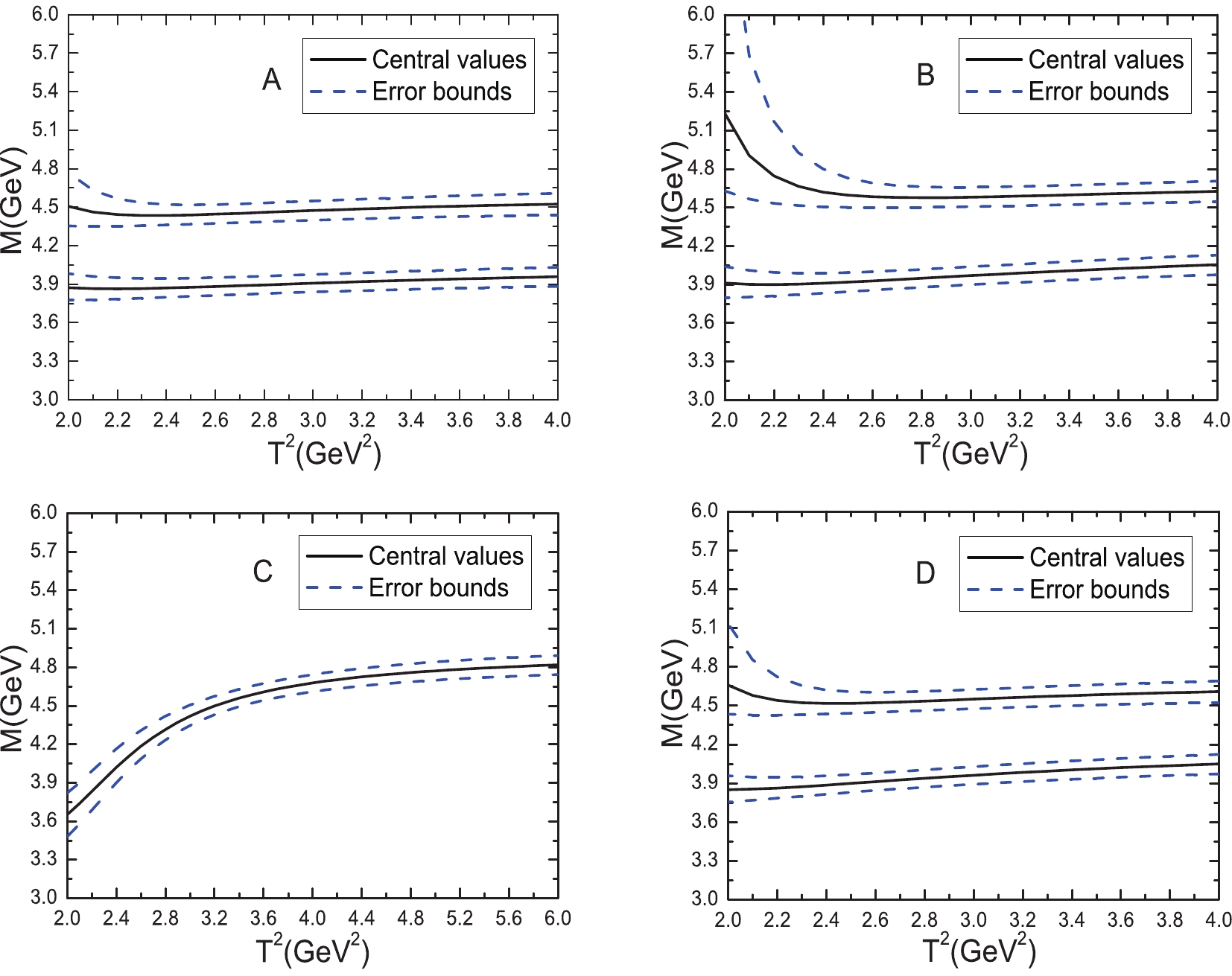
Figure 3. (color online) Masses with variations of Borel parameters
$T^2$ for axialvector hidden-charm tetraquark states, A, B, C, and D represent the$[uc]_S[\bar{d}\bar{c}]_A-[uc]_A[\bar{d}\bar{c}]_S$ ,$[uc]_{\tilde{A}}[\bar{d}\bar{c}]_A-[uc]_A[\bar{d}\bar{c}]_{\tilde{A}}$ ,$[uc]_{\tilde{V}}[\bar{d}\bar{c}]_V+[uc]_V[\bar{d}\bar{c}]_{\tilde{V}}$ , and$[uc]_A[\bar{d}\bar{c}]_A $ tetraquark states, respectively.The predicted mass
$ M_{Z} = 3.90\pm0.08\,\rm{GeV} $ for the ground state tetraquark state$[uc]_S[\bar{d}\bar{c}]_A- $ $ [uc]_A[\bar{d}\bar{c}]_S $ exhibits a good agreement with the experimental value$ M_{Z(3900)} = (3899.0\pm 3.6\pm 4.9)\,\rm{ MeV} $ from the BESIII collaboration [4], which is in favor of assigning the$ Z_c(3900) $ to the ground state tetraquark state$[uc]_S[\bar{d}\bar{c}]_A- $ $ [uc]_A[\bar{d}\bar{c}]_S $ with the quantum numbers$ J^{PC} = 1^{+-} $ [20]. In Ref. [45], we study the non-leptonic decays$Z_c^+(3900)\to $ $ J/\psi\pi^+ $ ,$ \eta_c\rho^+ $ ,$ D^+ \bar{D}^{*0} $ ,$ \bar{D}^0 D^{*+} $ with the three-point QCD sum rules. In analytical calculations, we consider both the factorizable and nonfactorizable Feynman diagrams, match the hadronic representation with the QCD representation according to solid quark-hadron duality, and obtain the total decay width$ \Gamma_{Z_c} = 54.2\pm29.8\,\rm{MeV} $ , which agrees with the experimental value$ (46\pm 10\pm 20) \,\rm{MeV} $ very well considering the uncertainties [4].The predicted mass
$ M_{Z} = 4.47\pm0.09\,\rm{GeV} $ for the first radially excited tetraquark state$ [uc]_S[\bar{d}\bar{c}]_A-[uc]_A[\bar{d}\bar{c}]_S $ exhibits good agreement with the experimental value$ M_{Z(4430)} = (4475\pm7\,{_{-25}^{+15}})\,\rm{ MeV} $ from the LHCb collaboration [10], which is in favor of assigning the$ Z_c(4430) $ to the first radially excited tetraquark state$ [uc]_S[\bar{d}\bar{c}]_A-$ $ [uc]_A[\bar{d}\bar{c}]_S $ with the quantum numbers$ J^{PC} = 1^{+-} $ . We investigate its non-leptonic decays with the three-point QCD sum rules to make a more reasonable assignment.The predicted mass
$ M_{Z} = 4.01\pm0.09\,\rm{GeV} $ for the ground state tetraquark state$ [uc]_{\tilde{A}}[\bar{d}\bar{c}]_A-[uc]_A[\bar{d}\bar{c}]_{\tilde{A}} $ and$ M_{Z} = 4.00\pm0.09\,\rm{GeV} $ for the ground state tetraquark state$ [uc]_A[\bar{d}\bar{c}]_A $ both exhibit good agreement with the experimental values$ M_{Z(4020/4025)} = (4026.3\pm2.6\pm3.7)\,\rm{MeV} $ [7] and$ (4022.9\pm 0.8\pm 2.7)\,\rm{MeV} $ [8] from the BESIII collaboration. There are two axialvector tetraquark state candidates with quantum numbers$ J^{PC} = 1^{+-} $ for$ Z_c(4020) $ . The two-body strong decays should be studied to make the assignment more reasonable.The predicted mass
$ M_{Z} = 4.60\pm0.09\,\rm{GeV} $ for the first radially excited tetraquark state$ [uc]_{\tilde{A}}[\bar{d}\bar{c}]_A-[uc]_A[\bar{d}\bar{c}]_{\tilde{A}} $ and$ M_{Z} = 4.58\pm0.09\,\rm{GeV} $ for the first radially excited tetraquark state$ [uc]_A[\bar{d}\bar{c}]_A $ both exhibit good agreement with the experimental value$ M_{Z(4600)} = 4600\,\rm{MeV} $ from the LHCb collaboration [1]. In contrast, the predicted mass$ M_{Z} = 4.66\pm0.10\,\rm{GeV} $ for the ground state tetraquark state$ [uc]_{\tilde{V}}[\bar{d}\bar{c}]_V+[uc]_V[\bar{d}\bar{c}]_{\tilde{V}} $ is also compatible with the experimental data$ M_{Z(4600)} = 4600\,\rm{MeV} $ from the LHCb collaboration [1]. Furthermore, the decay$ Z_c(4600)\to J/\psi \pi $ can take place more easily for the ground state tetraquark state, which is in good agreement with the observation of the$ Z_c(4600) $ in the$ J/\psi\pi $ invariant mass spectrum [1]. In summary, there are three axialvector tetraquark state candidates with$ J^{PC} = 1^{+-} $ for the$ Z_c(4600) $ , and further theoretical and experimental studies are required to identify$ Z_c(4600) $ unambiguously.In Ref. [2], we identify
$ Z_c(4600) $ as the$ [dc]_P[\bar{u}\bar{c}]_A- $ $[dc]_A[\bar{u}\bar{c}]_P $ type vector tetraquark state tentatively according to the predicted mass$ M_Z\!= \!(4.59\! \pm\! 0.08)\,\rm{GeV} $ from the QCD sum rules [46], and explore its non-leptonic decays$ Z_c(4600) \to J/\psi \pi $ ,$ \eta_c \rho $ ,$ J/\psi a_0 $ ,$ \chi_{c0} \rho $ ,$ D^*\bar{D}^* $ ,$ D\bar{D} $ ,$ D^*\bar{D} $ and$ D\bar{D}^* $ with QCD sum rules by matching the hadronic representation with the QCD representation with solid quark-hadron duality. The large partial decay width$ \Gamma(Z_c^-(4600)\to J/\psi \pi^-) = 41.4^{+20.5}_{-14.9}\,\rm{MeV} $ exhibits good agreement with the observation of the$ Z_c(4600) $ in the$ J/\psi \pi^- $ invariant mass spectrum.In Table 3, we present the diquark spin
$ S_{uc} $ , antidiquark spin$ S_{\bar{d}\bar{c}} $ , and total spin S of the hidden-charm tetraquark states. Table 3 shows that the$ [uc]_{\tilde{A}}[\bar{d}\bar{c}]_A- $ $[uc]_A[\bar{d}\bar{c}]_{\tilde{A}} $ and$ [uc]_A[\bar{d}\bar{c}]_A $ tetraquark states (that have tetraquark structures$ |1^+, 1; 1\rangle-|1, 1^+; 1\rangle $ and$ |1, 1; 1\rangle $ , respectively) have slightly larger masses than the$ [uc]_S[\bar{d}\bar{c}]_A-[uc]_A[\bar{d}\bar{c}]_S $ tetraquark state (which has the structure$ |0, 1; 1\rangle-|1, 0; 1\rangle $ ). This is reasonable, as the most favored diquark configurations or quark-quark correlations from the attractive interaction in the color-antitriplet (color-triplet) channel induced by one-gluon exchange are the scalar diquark (antidiquark) states. In previous studies, the scalar, pseudoscalar, vector, and axialvector diquarks states were investigated with the QCD sum rules, the scalar and axialvector heavy diquark states in the color-antitriplet have almost degenerate masses, or have almost the same typical quark-quark correlation lengths, the mass gaps between the scalar and axialvector heavy diquark states are very small or tiny [33]. Furthermore, this agrees with the predictions of the simple constituent diquark-antidiquark model [27].The vector (or P-wave) diquark states
$ [uc]_V $ and$ [uc]_{\tilde{V}} $ are expected to have larger masses than the axialvector (or S-wave) diquark states$ [uc]_A $ and$ [uc]_{\tilde{A}} $ , as there is a relative P-wave between the light and heavy quark. In the case of the traditional$ c\bar{u} $ charmed mesons, the energy exciting a P-wave costs about$ 458\,\rm{MeV} $ from the Particle Data Group [9],$\frac{{5{m_{D_2^*}} + 3{m_{{D_1}}} + {m_{D_0^*}}}}{9} - \frac{{3{m_{{D^*}}} + {m_D}}}{4} = 458 \;{\rm{MeV}} .$

(31) If the energy exciting a P-wave in the qc diquark systems also costs approximately
$ 458\;\rm{MeV} $ , the$[uc]_{\tilde{V}}[\bar{d}\bar{c}]_V+ $ $ [uc]_V[\bar{d}\bar{c}]_{\tilde{V}} $ tetraquark state has the largest ground state mass, which is even larger than the masses of the first radially excited states of the hidden-charm tetraquark states$ [uc]_{\tilde{A}}[\bar{d}\bar{c}]_A-[uc]_A[\bar{d}\bar{c}]_{\tilde{A}} $ and$ [uc]_A[\bar{d}\bar{c}]_A $ with the quantum numbers$ J^{PC} = 1^{+-} $ , as exciting two P-waves costs about$ 0.9\,\rm{GeV} $ , which is larger than the energy gap$ 0.6\,\rm{GeV} $ between the ground state hidden-charm tetraquark state and the first radial excitation of the hidden-charm tetraquark states. -
We investigate the ground states and the first radially excited states of the
$ [uc]_S[\bar{d}\bar{c}]_A-[uc]_A[\bar{d}\bar{c}]_S $ type,$ [uc]_{\tilde{A}}[\bar{d}\bar{c}]_A-[uc]_A[\bar{d}\bar{c}]_{\tilde{A}} $ type, and$ [uc]_A[\bar{d}\bar{c}]_A $ type tetraquark states and the ground state$ [uc]_{\tilde{V}}[\bar{d}\bar{c}]_V+ $ $ [uc]_V[\bar{d}\bar{c}]_{\tilde{V}} $ type tetraquark state with the quantum numbers$ J^{PC} = 1^{+-} $ using QCD sum rules in a systematic manner. The predicted tetraquark masses are in favor of assigning$ Z_c(3900) $ and$ Z_c(4430) $ as the ground state and the first radially excited state of the$ [uc]_S[\bar{d}\bar{c}]_A- $ $ [uc]_A[\bar{d}\bar{c}]_S $ type axialvector tetraquark states, respectively;$ Z_c(4020) $ as the ground state$ [uc]_{\tilde{A}}[\bar{d}\bar{c}]_A- $ $[uc]_A[\bar{d}\bar{c}]_{\tilde{A}} $ type axialvector tetraquark state or$ [uc]_A[\bar{d}\bar{c}]_A $ type axialvector tetraquark state;$ Z_c(4600) $ as the first radially excited$[uc]_{\tilde{A}}[\bar{d}\bar{c}]_A- $ $ [uc]_A[\bar{d}\bar{c}]_{\tilde{A}} $ type axialvector tetraquark state or$ [uc]_A[\bar{d}\bar{c}]_A $ type axialvector tetraquark state, or the ground state$ [uc]_{\tilde{V}}[\bar{d}\bar{c}]_V+[uc]_V[\bar{d}\bar{c}]_{\tilde{V}} $ type axialvector tetraquark state. Further experimental and theoretical studies are requiered to identify the$ Z_c(4600) $ unambiguously.
Axialvector tetraquark candidates for Zc(3900), Zc(4020), Zc(4430), and Zc(4600)
- Received Date: 2019-11-21
- Accepted Date: 2020-02-17
- Available Online: 2020-06-01
Abstract: We construct the axialvector and tensor current operators to systematically investigate the ground and first radially excited tetraquark states with quantum numbers


 DownLoad: