


 Abstract
 HTML
HTML Reference
 Related
 PDF
PDF


-
Exotic states cannot be described by the traditional quark model and may have a more complex structure allowed by QCD such as glueballs, hybrid mesons and multiquark states. The discovery of exotic states and the study of their structure will extend our knowledge of the strong interaction dynamics [1-3].
A meson with quantum numbers
$ J^{PC} = 1^{-+} $ , which is excluded by the traditional quark model in the$ q \bar{q} $ picture, is an exotic state [4]. Interestingly, three isovector$ J^{PC} = 1^{-+} $ exotic candidates,$ \pi_1(1400) $ ,$ \pi_1(1600) $ , and$ \pi_1(2015) $ , have been reported by experiments [5]. On the theoretical side, the isovector exotic states are interpreted as hybrid mesons in different theoretical approaches, such as the flux tube model [6-8], ADS/QCD model [9, 10], and Lattice QCD [11-13]. In addition, the hybrid meson decay properties were studied in the framework of the QCD sum rules in Refs. [14-17]. Some studies suggest that the isovector exotic state might be a four-quark state [18] or a molecule/four-quark mixing state [19]. On the other hand, the three-body system can also carry the quantum numbers$ J^{PC} = 1^{-+} $ . In Ref. [20], by retaining the strong interactions of$ \bar{K}K^* $ which generate the$ f_1(1285) $ resonance [21, 22], the$ \pi \bar{K}K^* $ three-body system was investigated in the framework of the fixed-center approximation (FCA) of the Faddeev equation, where$ \pi_1(1600) $ could be interpreted as a dynamically generated state in the$ \pi $ -$ (\bar{K}K^*)_{f_1(1285)} $ system.In principle, an isoscalar exotic state is also possible, although it has not been experimentally observed [8, 13]. In fact, these isoscalar exotic states were studied with the QCD sum rules using the tetraquark currents [23], where the obtained mass is around
$ 1.8 \sim 2.1 $ GeV, and the decay width is about 150 MeV.In this paper, we study the
$ \eta \bar{K}K^* $ three-body system in order to look for possible$ I^G(J^{PC}) = 0^+(1^{-+}) $ exotic states in the FCA approach, which has been used to investigate the interaction of$ K^-d $ at the threshold [24-26]. A possible state in the three-body system$ K^- pp $ , according to calculations performed with the FCA approach [27, 28], is supported by the J-PARC experiments [29]. In Ref. [30], the$ \Delta_{5/2^+}(2000) $ puzzle is solved in a study of the$ \pi $ -$ (\Delta \rho) $ interaction. In Ref. [31], a peak is found around 1920 MeV, indicating that the$ NK \bar{K} $ state with$ I = 1/2 $ could exists around that energy, which supports the existence of the$ N^* $ resonance with$ J^P = 1/2^+ $ around 1920 MeV obtained in Refs. [32-35], where the full Faddeev calculations were performed. Recently, predictions of several heavy flavor resonance states in a three-body system have been reported in the framework of the FCA approach, for example$ \bar{K}^{(*)} B^{(*)}\bar{B}^{(*)} $ [36],$ D^{(*)}B^{(*)}\bar{B}^{(*)} $ [37],$ \rho B^* \bar{B}^* $ [38],$ \rho D^* \bar{D}^* $ [39, 40],$ DKK $ $ (DK\bar{K}) $ [41],$ BDD (BD\bar{D}) $ [42], and$ K\bar{D}D^* $ [43]. The$ DDK $ system was investigated in Ref. [44] with coupled channels by solving the Faddeev equation using the two-body input, and it was found that an isospin 1/2 state is formed at 4140 MeV when$ D^*_{s0}(2317) $ is formed in the$ DK $ subsystem. This result is compatible with Ref. [45], where the system D-$ D^*_{s0}(2317) $ was studied without the explicit three-body dynamics. In a more recent work [46], where the Gaussian expansion method was used, the existence of$ DDK $ states was further confirmed. The above examples show that the results of FCA prove to be reasonable. However, as important as it may be to understand the success of FCA, there are problems in the FCA calculations of the$ \phi K \bar{K} $ system [47] (more details about the limits of FCA can also be found in this reference), in which$ \phi(2175) $ can be reproduced by the full Faddeev calculations [48].There are two possible scattering cases in the
$ \eta \bar{K}K^* $ three-body system since the$ \bar{K}K^* $ and$ \eta K^* $ systems lead to the formation of two dynamically generated resonances,$ f_1(1285) $ and$ K_1(1270) $ . Based on the two-body$ \eta \bar{K} $ ,$ \eta K^* $ and$ \bar{K}K^* $ scattering amplitudes obtained from the chiral unitary approach [21, 49, 50], we perform an analysis of the$ \eta $ -$ (\bar{K}K^*)_{f_1(1285)} $ and$ \bar{K} $ -$ (\eta K^*)_{K_1(1270)} $ scattering amplitudes, which allows to predict the possible exotic states with quantum numbers$I^G(J^{PC}) = $ $ 0^+(1^{-+}) $ .The paper is organized as follows. In Sec. 2, we present the FCA formalism and ingredients to analyze the
$ \eta $ -$ (\bar{K}K^*)_{f_1(1285)} $ and$ \bar{K} $ -$ (\eta K^*)_{K_1(1270)} $ systems. In Sec. 3, numerical results and a discussion are presented. Finally, a short summary is given in Sec. 4. -
In the framework of FCA, we consider
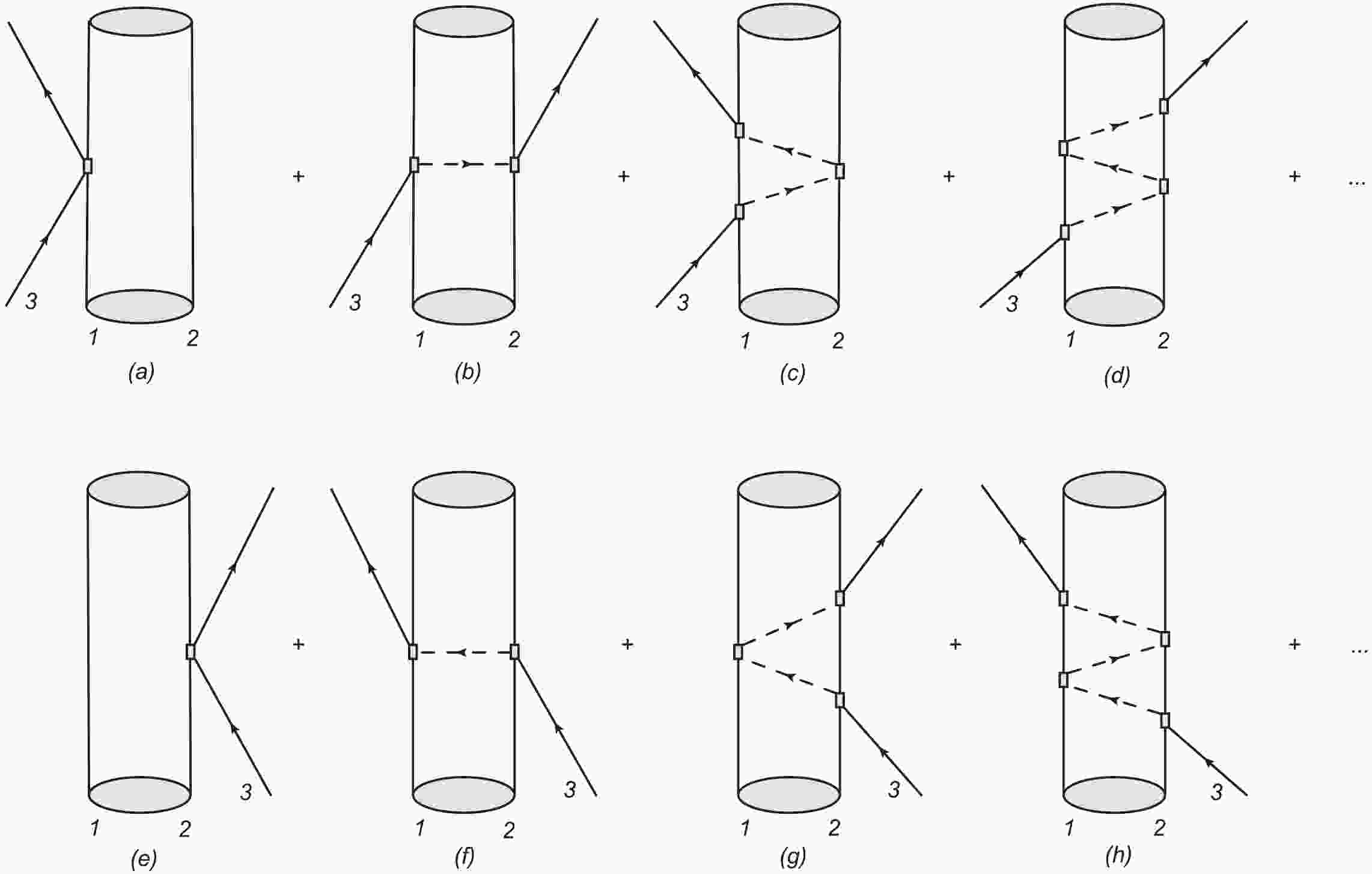
$ \bar{K}K^*(\eta K^*) $ as a cluster, and$ \eta(\bar{K}) $ interacts with the components of the cluster. The total three-body scattering amplitude$ T $ can be simplified as the sum of two partition functions$ T_1 $ and$ T_2 $ , by summing all diagrams in Fig. 1, starting with the interaction of particle 3 with particle 1(2) of the cluster. The FCA equations can be written in terms of$ T_1 $ and$ T_2 $ , which give the total scattering amplitude$ T $ , and read [25, 26, 51]
Figure 1. Diagrammatic representation of FCA for the Faddeev equations.
$ T_1 = t_1+t_1G_0T_2, $

(1) $ T_2 = t_2+t_2G_0T_1, $

(2) $ T = T_1+T_2, $

(3) where the amplitudes
$ t_1 $ and$ t_2 $ represent the unitary scattering amplitudes with coupled channels for the interactions of particle 3 with particle 1 and 2, respectively. The function$ G_0 $ in the above equations is the propagator for particle 3 between the particle 1 and 2 components of the cluster, which we discuss below.We calculate the total scattering amplitude
$ T $ in the low energy regime, close to the threshold of the$ \eta \bar{K} K^* $ system or below, where FCA is a good approximation. The on-shell approximation for the three particles is also used.Following the field normalization of Refs. [52, 53], we can write the
$ S $ matrix for the single scattering term [Fig. 1(a) and 1(e)] as①$\begin{split} S^{(1)} =& S_1^{(1)}+S_2^{(1)} = \frac{(2\pi)^4}{{\cal{V}}^2}\delta^4(k_3+k_{\rm{cls}}-k_3'-k_{\rm{cls}}') \\ &\times\frac{1}{\sqrt{2w_3}}\frac{1}{\sqrt{2w_3'}} \left(\frac{-{\rm i}t_1}{\sqrt{2w_1}} \frac{1}{\sqrt{2w_1'}} + \frac{-{\rm i}t_2}{\sqrt{2w_2}} \frac{1}{\sqrt{2w_2'}}\right), \end{split}$

(4) where
$ {\cal{V}} $ stands for the volume of a box in which the states are normalized to unity, while the momentum$ k(k') $ and the on-shell energy$ w(w') $ refer to the initial (final) particles.The double scattering contributions are obtained from Fig. 1(b) and 1(f). The expression for the
$ S $ matrix for double scattering [$ S_2^{(2)} = S_1^{(2)} $ ] is given by$ \begin{split} S^{(2)} =& -{\rm i}t_1t_2\frac{(2\pi)^4}{{\cal{V}}^2} \delta^4(k_3+k_{\rm{cls}}-k_3'-k_{\rm{cls}}') \\ & \times\frac{1}{\sqrt{2w_3}} \frac{1}{\sqrt{2w_3'}} \frac{1}{\sqrt{2w_1}} \frac{1}{\sqrt{2w_1'}} \frac{1}{\sqrt{2w_2}} \frac{1}{\sqrt{2w_2'}} \\& \times \int \frac{{\rm d}^3q}{(2\pi)^3} F_{\rm{cls}}(q) \frac{1}{{q^0}^2-|{\vec{q}}|^2-m_3^2+{\rm i} \epsilon}, \end{split}$

(5) where
$ F_{\rm{cls}}(q) $ is the form factor of the cluster which is a bound state of particles 1 and 2. The information about the bound state is encoded in the form factor$ F_{\rm{cls}}(q) $ in Eq. (5), which is the Fourier transform of the cluster wave function. The variable$ q^0 $ is the energy carried by particle 3 in the center-of-mass frame of particle 3 and the cluster, and is given by$ q^0(s) = \frac{s+m_3^2-m_{\rm{cls}}^2}{2\sqrt{s}}, $

(6) where
$ s $ is the invariant mass squared of the$ \eta \bar{K} K^* $ system.For the form factor
$ F_{\rm{cls}}(q) $ , we take the following expression for$ s $ wave bound states only, as discussed in Refs. [52-54]:$ \begin{split} F_{\rm{cls}}(q) = &\frac{1}{N}\int_{\vert \vec{p} \vert < \Lambda,\vert \vec{p}-\vec{q} \vert < \Lambda} {\rm d}^3 \vec{p} \; \frac{1}{2w_1(\vec{p})}\frac{1}{2w_2(\vec{p})} \\& \times\frac{1}{m_{\rm{cls}}-w_1(\vec{p})-w_2(\vec{p})} \frac{1}{2w_1(\vec{p}-\vec{q})}\frac{1}{2w_2(\vec{p}-\vec{q})} \\& \times\frac{1}{m_{\rm{cls}}-w_1(\vec{p}-\vec{q})-w_2(\vec{p}-\vec{q})}, \end{split} $

(7) where the normalization factor
$ N $ is$ N = \int_{\vert \vec{p} \vert < \Lambda} {\rm d}^3 \vec{p} \; \left( \frac{1}{2w_1(\vec{p})}\frac{1}{2w_2(\vec{p})} \frac{1}{m_{\rm{cls}}-w_1(\vec{p})-w_2(\vec{p})}\right)^2, $

with
$ m_{\rm{cls}} $ the mass of the cluster. Note that the width of$ K^* $ should also be included in$ F_{\rm{cls}}(q) $ [30]. However, as shown below, the masses of$ f_1(1285) $ and$ K_1(1270) $ are below the threshold of$ \bar{K}K^* $ and$ \eta K^* $ , and the effect of the width of$ K^* $ is small and can be neglected.Similarly, the full
$ S $ matrix for the scattering of particle 3 on the cluster is given by$ \begin{split} S =& -{\rm i}T\frac{(2\pi)^4}{{\cal{V}}^2}\delta^4(k_3+k_{\rm{cls}}-k_3'-k_{\rm{cls}}') \\ &\times\frac{1}{\sqrt{2w_3}} \frac{1}{\sqrt{2w_3'}} \frac{1}{\sqrt{2w_{\rm{cls}}}} \frac{1}{\sqrt{2w_{\rm{cls}}'}}. \end{split} $

(8) By comparing Eqs. (4), (5), and (8), we see that it is necessary to introduce a weight in
$ t_1 $ and$ t_2 $ so that Eqs. (4) and (5) include the factors that appear in Eq. (8). This is achieved by,$ \begin{align} \tilde{t}_1 = t_1\sqrt{\frac{2w_{\rm{cls}}}{2w_1}}\sqrt{\frac{2w_{\rm{cls}}'}{2w_1'}}, \; \; \; \; \; \; \tilde{t}_2 = t_2\sqrt{\frac{2w_{\rm{cls}}}{2w_2}}\sqrt{\frac{2w_{\rm{cls}}'}{2w_2'}}. \end{align} $

Eq. (3) can then be solved to give
$ \begin{align} T = \frac{\tilde{t}_1+\tilde{t}_2+2\tilde{t}_1\tilde{t}_2G_0}{1-\tilde{t}_1\tilde{t}_2G_0^2}, \end{align} $

(9) where
$ G_0 $ depends on the invariant mass of the$ \eta \bar{K}K^* $ system, and is given by$ G_0(s) = \frac{1}{2m_{\rm{cls}}}\int \frac{{\rm d}^3q}{(2\pi)^3} \frac{F_{\rm{cls}}(q)}{{q^0}^2 - |\vec{q}\; |^2-m_3^2+{\rm i} \epsilon} . $

(10) -
It is worth noting that the argument of the total scattering amplitude
$ T $ can be regarded as a function of the total invariant mass$ \sqrt{s} $ of the three-body system, while the arguments of two-body scattering amplitudes$ t_1 $ and$ t_2 $ depend on the two-body invariant masses$ \sqrt{s_1} $ and$ \sqrt{s_2} $ .$ s_1 $ and$ s_2 $ are the invariant masses squared of the external particle$ 3 $ with momentum$ k_3 $ , and particle 1 (2) inside the cluster with momentum$ k_1 $ ($ k_2 $ ), which are given by$ \begin{split} s_1 =& m_3^2+m_1^2+\frac{(s-m_3^2-m_{ \rm{\rm{cls}}}^2)(m_{\rm{cls}}^2+m_1^2-m_2^2)}{2m_{\rm{cls}}^2}, \\ s_2 =& m_3^2+m_2^2+\frac{(s-m_3^2-m_{\rm{cls}}^2)(m_{\rm{cls}}^2+m_2^2-m_1^2)}{2m_{\rm{cls}}^2}, \end{split} $

where
$ m_l $ $ (l = 1,2,3) $ are the masses of the corresponding particles in the three-body system.It is worth mentioning that in order to evaluate the two-body scattering amplitudes
$ t_1 $ and$ t_2 $ , the isospin of the cluster should be considered. For the case of the$ \eta $ -$ (\bar{K}K^*)_{f_1(1285)} $ system, the cluster$ \bar{K}K^* $ has isospin$ I_{\bar{K}K^*} = 0 $ . Therefore, we have$ \begin{align} \vert \bar{K} K^* \rangle_{I = 0} = \frac{1}{\sqrt{2}}\left| \left(\frac{1}{2} ,-\frac{1}{2}\right) \right\rangle-\frac{1}{\sqrt{2}}\left| \left(-\frac{1}{2} ,\frac{1}{2} \right)\right\rangle, \end{align} $

(11) where the kets on the right-hand side indicate the
$ I_z $ components of particles$ \bar{K} $ and$ K^* $ ,$ \vert (I_z^{\bar{K}} ,I_z^{K^*} )\rangle $ . For the case of the total isospin$ I_{\eta(\bar{K}K^*)} = 0 $ , the single scattering amplitude is written as [20]$ \begin{split} \langle \eta(\bar{K}K^*)\vert t \vert \eta(\bar{K}K^*) \rangle =&\Bigg( \langle0 0 \vert \otimes \frac{1}{\sqrt{2}}\Bigg( \Bigg\langle \Bigg(\frac{1}{2} ,-\frac{1}{2}\Bigg) \Bigg\vert - \Bigg\langle \Bigg(-\frac{1}{2} ,\frac{1}{2}\Bigg)\Bigg \vert \Bigg) \Bigg) (t_{31}+t_{32}) \Bigg( \vert 0 0 \rangle \otimes \frac{1}{\sqrt{2}}\Bigg( \Bigg\vert \Bigg(\frac{1}{2} ,-\frac{1}{2}\Bigg) \Bigg\rangle - \Bigg\vert \Bigg(-\frac{1}{2} ,\frac{1}{2} \Bigg)\Bigg\rangle \Bigg) \Bigg) \\ =& \Bigg( \frac{1}{\sqrt{2}} \Bigg\langle \Bigg(\frac{1}{2}\frac{1}{2},-\frac{1}{2}\Bigg) \Bigg\vert - \frac{1}{\sqrt{2}}\Bigg\langle \Bigg(\frac{1}{2}\!\!-\!\!\frac{1}{2},\frac{1}{2}\Bigg)\Bigg \vert \Bigg) t_{31} \Bigg( \frac{1}{\sqrt{2}}\Bigg \vert \Bigg(\frac{1}{2}\frac{1}{2},-\frac{1}{2}\Bigg)\Bigg \rangle - \frac{1}{\sqrt{2}} \Bigg\vert \Bigg(\frac{1}{2}\!\!-\!\!\frac{1}{2},\frac{1}{2}\Bigg)\Bigg \rangle \Bigg) \\ &+\Bigg( \frac{1}{\sqrt{2}}\Bigg\langle \Bigg(\frac{1}{2}\frac{1}{2},-\frac{1}{2}\Bigg) \Bigg\vert - \frac{1}{\sqrt{2}}\Bigg\langle \Bigg(\frac{1}{2}\!\!-\!\!\frac{1}{2},\frac{1}{2}\Bigg) \Bigg\vert \Bigg) t_{32} \Bigg( \frac{1}{\sqrt{2}}\Bigg \vert \Bigg(\frac{1}{2} \!\!-\!\!\frac{1}{2},\frac{1}{2}\Bigg) \Bigg\rangle - \frac{1}{\sqrt{2}} \Bigg\vert \Bigg(\frac{1}{2}\frac{1}{2},-\frac{1}{2}\Bigg) \Bigg\rangle \Bigg) , \end{split} $

(12) where the notation for the states in the last term is
$ \vert(I_{\eta \bar{K}}I_{\eta \bar{K}}^z,I_{K^*}^z)\rangle $ for$ t_{31} $ and$ \vert(I_{\eta K^*}I_{\eta K^*}^z,I_{\bar{K}}^z)\rangle $ for$ t_{32} $ . This leads to the following amplitudes for single scattering [Fig. 1(a) and 1(e)] in the$ \eta $ -$ (\bar{K}K^*)_{f_1(1285)} $ system,$ \begin{align} t_1 = t_{\eta \bar{K} \to \eta \bar{K}}^{I = 1/2}, \quad t_2 = t_{\eta K^* \to \eta K^*}^{I = 1/2}. \end{align} $

(13) In the
$ \bar{K} $ -$ (\eta K^*)_{K_1(1270)} $ system, the cluster$ \eta K^* $ can only have isospin$ I_{\eta K^*} = 1/2 $ . Therefore, for the total isospin$ I_{\bar{K}(\eta K^*)} = 0 $ , the scattering amplitude is written as [20]$\begin{split} \langle \bar{K}(\eta K^*)\vert t \vert \bar{K}(\eta K^*) \rangle = & \frac{1}{\sqrt{2}} \Bigg( \Bigg\langle\frac{1}{2} \frac{1}{2} \vert \otimes \Bigg\langle \Bigg(\frac{1}{2} ,-\frac{1}{2}\Bigg) \Bigg\vert - \Bigg\langle\frac{1}{2} \!\!-\!\!\frac{1}{2} \Bigg\vert \otimes \Bigg\langle \Bigg(\frac{1}{2} ,\frac{1}{2}\Bigg)\Bigg \vert \Bigg) (t_{31}+t_{32}) \frac{1}{\sqrt{2}} \Bigg( \Bigg\vert \frac{1}{2} \frac{1}{2} \Bigg\rangle \otimes \Bigg\vert \Bigg(\frac{1}{2} ,-\frac{1}{2}\Bigg) \Bigg\rangle - \Bigg\vert \frac{1}{2} \!\!-\!\!\frac{1}{2} \Bigg\rangle \otimes \Bigg\vert \Bigg(\frac{1}{2} ,\frac{1}{2} \Bigg)\Bigg\rangle \Bigg) \\ =& \Bigg( \frac{1}{\sqrt{2}} \Bigg\langle \Bigg(\frac{1}{2}\frac{1}{2},-\frac{1}{2}\Bigg) \Bigg\vert - \frac{1}{\sqrt{2}}\Bigg\langle \Bigg(\frac{1}{2}\!\!-\!\!\frac{1}{2},\frac{1}{2}\Bigg)\Bigg \vert \Bigg) t_{31} \Bigg( \frac{1}{\sqrt{2}}\Bigg \vert \Bigg(\frac{1}{2}\frac{1}{2},-\frac{1}{2}\Bigg)\Bigg \rangle - \frac{1}{\sqrt{2}} \Bigg\vert \Bigg(\frac{1}{2}\!\!-\!\!\frac{1}{2},\frac{1}{2}\Bigg)\Bigg \rangle \Bigg) \\& +\frac{1}{\sqrt{2}}\Bigg( \frac{1}{\sqrt{2}}\Bigg\langle (00,0) + \frac{1}{\sqrt{2}}\Bigg\langle (00,0) \Bigg\vert \Bigg) t_{32} \frac{1}{\sqrt{2}}\Bigg( \frac{1}{\sqrt{2}} \Bigg\vert (00,0)\Bigg \rangle + \frac{1}{\sqrt{2}} \Bigg\vert (00,0) \Bigg\rangle \Bigg). \end{split} $

(14) This leads to the following amplitudes for single scattering in the
$ \bar{K} $ -$ (\eta K^*)_{K_1(1270)} $ system,$ \begin{align} t_1 = t_{\bar{K} \eta \to \bar{K} \eta}^{I = 1/2}, \quad t_2 = t_{\bar{K} K^* \to \bar{K} K^*}^{I = 0}. \end{align} $

(15) We see that only the transition
$ \bar{K}K^* \to \bar{K}K^* $ with$ I = 0 $ gives a contribution, since the total isospin$ I_{\bar{K}(\eta K^*)} = 0 $ and the$ \eta $ meson has isospin zero. -
An important ingredient in the calculations of the total scattering amplitude for the
$ \eta \bar{K} K^* $ system using FCA are the two-body$ \eta K $ ,$ \eta K^* $ , and$ \bar{K} K^* $ unitarized$ s $ wave interactions from the chiral unitary approach. These two-body scattering amplitudes are studied with the dimensional regularization procedure, and they depend on the subtraction constants$ a_{\eta K} $ ,$ a_{\eta K^*} $ and$ a_{\bar{K}K^*} $ , and also on the regularization scale$ \mu $ . Note that there is only one parameter for the dimensional regularization procedure, since any change in$ \mu $ is reabsorbed by the change in$ a(\mu) $ through$ a(\mu') - a(\mu) = {\rm ln}(\frac{\mu'^2}{\mu^2}) $ , so that the scattering amplitude is scale independent. In this work, we use the parameters from Refs. [21, 49, 50]:$ a_{\eta K} = -1.38 $ and$ \mu = m_K $ for$ I_{\eta K} = 1/2 $ ;$ a_{\eta K^*} = -1.85 $ and$ \mu = 1000 $ MeV for$ I_{\eta K^*} = 1/2 $ ;$ a_{\bar{K}K^*} = -1.85 $ and$ \mu = 1000 $ MeV for$ I_{\bar{K}K^*} = 0 $ . With these parameters, we get the masses of$ f_1(1285) $ and$ K_1(1270) $ at their estimated values.In Figs. 2(a) and (b), we show the numerical results for
$ |t_{\bar{K} K^* \to \bar{K} K^*}^{I = 0}|^2 $ and$ |t_{\eta K^* \to \eta K^*}^{I = 1/2}|^2 $ , respectively, where we see clear peaks for the$ f_1(1285) $ and$ K_1(1270) $ states.
Figure 2. (a) Modulus squared of
$ t_{\bar{K} K^* \to \bar{K} K^*}^{I = 0} $ as a function of the invariant mass$ M_{\bar{K}K^*} $ of the$ \bar{K}K^* $ subsystem. (b) Modulus squared of$ t_{\eta K^* \to \eta K^*}^{I = 1/2} $ as a function of the invariant mass$ M_{\eta K^*} $ of the$ \eta K^* $ subsystem. -
To connect with the dimensional regularization procedure, we choose the cutoff
$ \Lambda $ such that the two-body loop function at the threshold coincides in both methods. Thus, we take$ \Lambda = 990 $ MeV such that$ f_1(1285) $ is as obtained in Refs. [55, 56], while for$ K_1(1270) $ , we take$ \Lambda = 1000 $ MeV. The cutoff is tuned to get a pole at$ 1288- i74 $ for the$ K_1(1270) $ state.In Figs. 3 and 4, we show the respective form-factors for
$ f_1(1285) $ and$ K_1(1270) $ , where we take$ m_{\rm{cls}} = 1281.3 $ MeV for$ f_1(1285) $ and 1284 MeV for$ K_1(1270) $ , as obtained in Ref. [49]. In FCA, we keep the wave function of the cluster unchanged in the presence of the third particle. In order to estimate the uncertainties of FCA due to this "frozen" condition, we admit that the wave function of the cluster could be modified by the presence of the third particle. To do so, we perform calculations with different cutoffs. The results, shown in Figs. 3 and 4, are obtained with$ \Lambda = 890 $ ,$ 990 $ and$ 1090 $ MeV for$ f_1(1285) $ , while for$ K_1(1270) $ we take$ \Lambda = 900 $ , 1000 and 1100 MeV.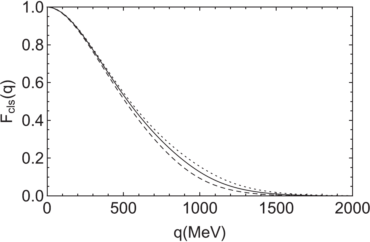
Figure 3. Forms-factor Eq. (7) as a function of
$ q = |\vec{q}\; | $ for the cutoff$ \Lambda = 890 $ (dashed),$ 990 $ (solid), and$ 1090 $ MeV (dotted) for$ f_1(1285) $ as the$ \bar{K}K^* $ bound state.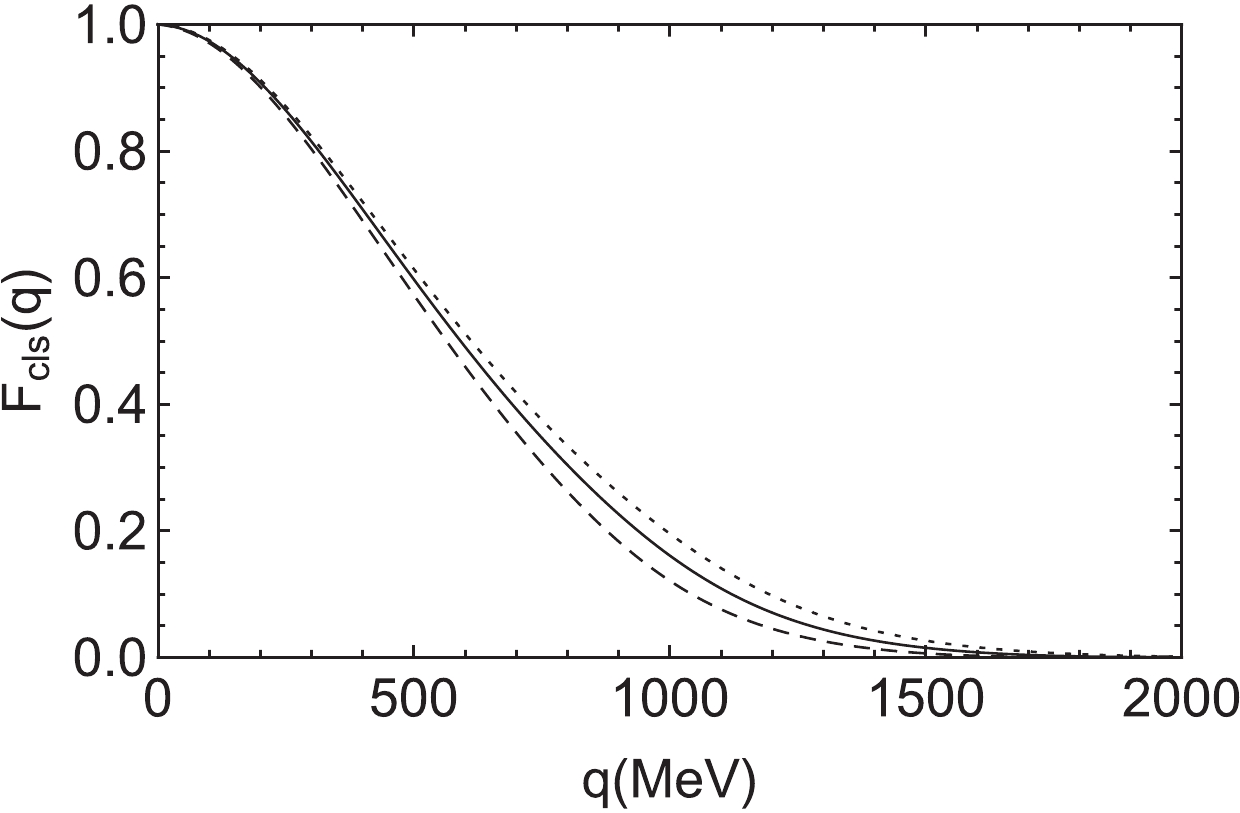
Figure 4. As in Fig. 3, but for
$ K_1(1270) $ as the$ \eta K^* $ bound state. The dashed, solid and dotted curves are for$ \Lambda = 900 $ , 1000, and 1100 MeV, respectively.In Fig. 5, we show the real (solid line) and imaginary (dashed line) parts of
$ G_0 $ as a function of the invariant mass of the$ \eta $ -$ (\bar{K}K^*)_{f_1(1285)} $ system for$ \Lambda = 890 $ ,$ 990 $ and$ 1090 $ MeV.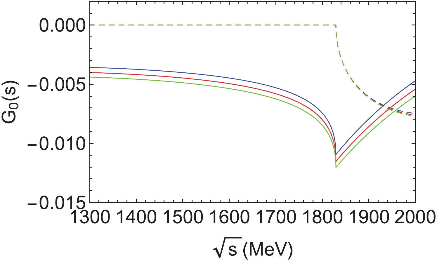
Figure 5. (color online) Real (solid line) and imaginary (dashed line) parts of
$ G_0 $ for the$ \eta $ -$ (\bar{K}K^*)_{f_1(1285)} $ system and$ \Lambda = 890 $ (blue),$ 990 $ (red) and$ 1090 $ MeV (green).The results for
$ G_0 $ of the$ \bar{K} $ -$ (\eta K^*)_{K_1(1270)} $ system are shown in Fig. 6, where the real (solid line) and imaginary (dashed line) parts are for$ \Lambda = 900 $ ,$ 1000 $ and$ 1100 $ MeV.From Figs. 5 and 6, it can be seen that the imaginary part of
$ G_0(s) $ is not sensitive to the value of the cutoff, while the real part slightly changes with the cutoff.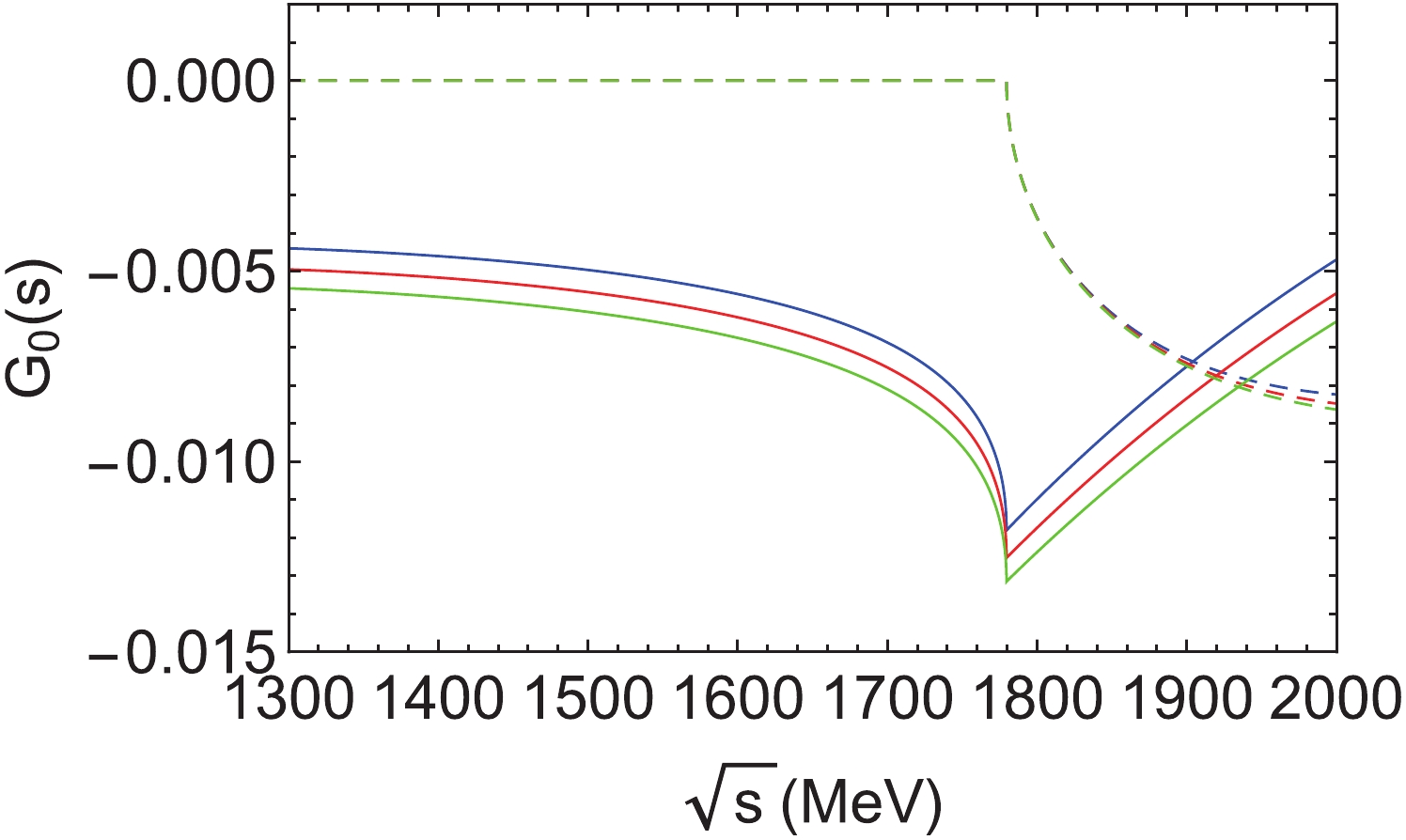
Figure 6. (color online) Real (solid line) and imaginary (dashed line) parts of
$ G_0 $ for the$ \bar{K} $ -$ (\eta K^*)_{K_1(1270)} $ system and$ \Lambda = 900 $ (blue),$ 1000 $ (red) and$ 1100 $ MeV (green). -
For the numerical evaluation of the three-body amplitude, we need the two-body interaction amplitudes of
$ \eta \bar{K} $ ,$ \eta K^* $ , and$ \bar{K} K^* $ , which were investigated in the chiral dynamics and unitary coupled channels approach in Refs. [21, 49, 50]. The total scattering amplitude$ T $ can then be calculated, and the peaks or bumps in the modulus squared$ \vert T \vert ^2 $ associated to resonances.In Fig. 7, we show the modulus squared
$ |T|^2 $ for the$ \eta $ -$ (\bar{K}K^*)_{f_1(1285)} $ scattering with the total isospin$ I = 0 $ . A clear bump structure can be seen below the$ \eta{f_1(1285)} $ threshold with a mass of around 1700 MeV and a width of about 180 MeV. Furthermore, taking$ \sqrt{s} = 1700 $ MeV, we get$ \sqrt{s_1} = 927 $ MeV and$ \sqrt{s_2} = 1315 $ MeV. At this energy, the interactions of$ \eta \bar{K} $ and$ \eta K^* $ are strong.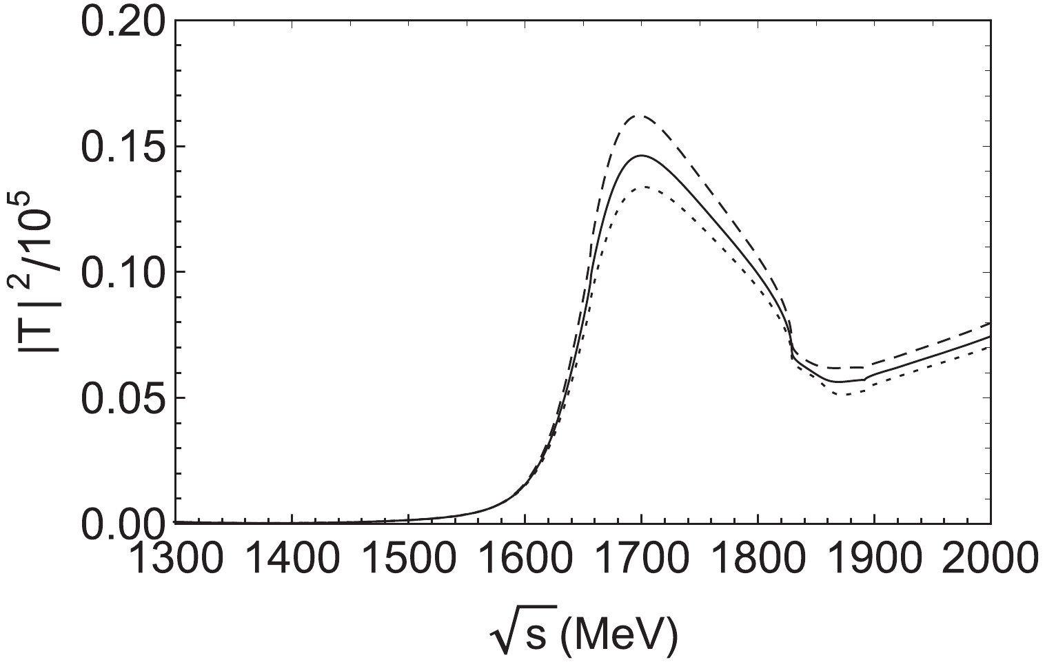
Figure 7. Modulus squared of the total amplitude
$ T $ for the$ \eta $ -$ (\bar{K}K^*)_{f_1(1285)} $ system. The dashed, solid and dotted curves are for$ \Lambda = 890, 990 $ , and$ 1090 $ MeV, respectively.In Fig. 8, we show
$ \vert T \vert ^2 $ for the$ \bar{K} $ -$ (\eta K^*)_{K_1(1270)} $ system. A strong resonant structure around 1680 MeV with a width of about 160 MeV is clearly seen, which indicates that the$ \bar{K} $ -$ (\eta K^*)_{K_1(1270)} $ state could be formed. The mass of this state is below the$ \bar{K} $ and$ {K_1(1270)} $ mass threshold. The strength of$ |T|^2 $ at the peak is much higher than in Fig. 7 for the$ \eta f_1(1285) \to \eta f_1(1285) $ scattering. Thus, it is clear that the preferred configuration is$ \bar{K} K_1(1270) $ . However,$ \bar{K} $ keeps interacting with$ K^* $ , and could sometimes also form$ f_1(1285) $ .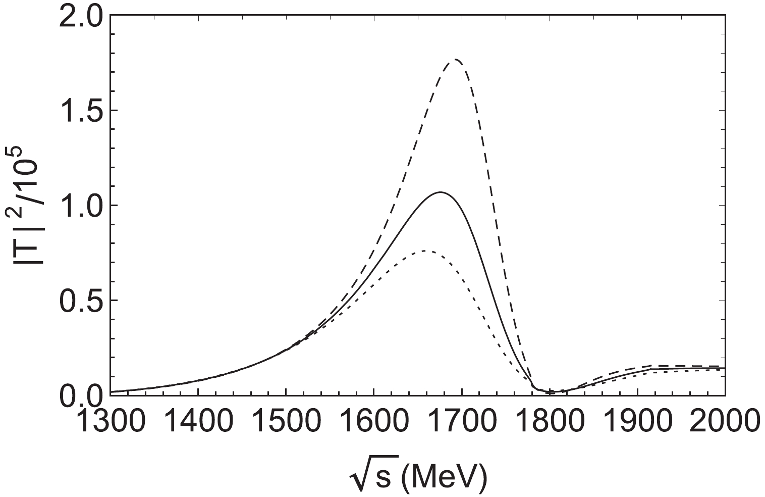
Figure 8. Modulus squared of the total amplitude
$ T $ for the$ \bar{K} $ -$ (\eta K^*)_{K_1(1270)} $ system. The dashed, solid and dotted curves are for$ \Lambda = 900, 1000 $ , and$ 1100 $ MeV, respectively.From Figs. 7 and 8, it can be seen that the peak positions and widths for the
$ \eta $ -$ (\bar{K}K^*)_{f_1(1285)} $ and$ \bar{K} $ -$ (\eta K^*)_{K_1(1270)} $ systems are quite stable for small variations of the cutoff parameter$ \Lambda $ . ② This gives confidence that the$ \eta $ -$ (\bar{K}K^*)_{f_1(1285)} $ and$ \bar{K} $ -$ (\eta K^*)_{K_1(1270)} $ bound states can be formed. In fact, the$ \eta f_1(1285) $ configuration could mix with$ \bar{K}K_1(1270) $ . However, since the strength of$ \bar{K} $ -$ (\eta K^*)_{K_1(1270)} $ scattering is much higher than of$ \eta $ -$ (\bar{K}K^*)_{f_1(1285)} $ scattering, the interference between the two configurations should be small. As both configurations peak around a similar energy, it is expected that the peak of any mixture of states is also around this energy.The
$ \eta \bar{K} K^* $ bound state with quantum numbers$ I(J^P) = 0 (1^-) $ has a dominant$ \bar{K}K_1(1270) $ component. Since$ K_1(1270) $ mostly decays into$ K \pi \pi $ [49], the dominant decay mode of the proposed state should be$ \bar{K}K\pi \pi $ , and we hope that future experimental measurements could test our predictions.We should mention that two
$ K_1(1270) $ states were obtained in Ref. [49]. The one with a mass of 1284 MeV couples more strongly to the$ \eta K^* $ and$ K \rho $ channels, while the other with a mass of 1195 MeV mainly couples to the$ \pi K^* $ channel, and couples very weakly to$ \eta K^* $ . Thus, one could expect that the lower mass$ K_1(1270) $ state of Ref. [49] does not affect our calculations. -
In this work, we used FCA of the Faddeev equation to look for possible
$ I^G(J^{PC}) = 0^+(1^{-+}) $ exotic states generated from the$ \eta\bar{K}K^* $ three-body interactions. We first selected a cluster$ \bar{K}K^* $ , which is known to generate$ f_1(1285) $ with$ I = 0 $ , and then allowed the$ \eta $ meson to interact with$ \bar{K} $ and$ K^* $ . In the modulus squared of the$ \eta $ -$ (\bar{K}K^*)_{f_1(1285)} $ scattering amplitude, we find evidence of a bound state below the$ \eta{f_1(1285)} $ threshold with a mass of around 1700 MeV and a width of about 180 MeV. In the case of$ \bar{K} $ scattering with the cluster$ \eta K^* $ , which was shown to generate$ K_1(1270) $ with$ I = 1/2 $ , we obtained a bound state$ I(J^{P}) = 0(1^{-}) $ just below the$ \bar{K}{K_1(1270)} $ threshold with a mass of around 1680 MeV and a width of about 160 MeV. In addition, the simplicity of the present approach also allows a transparent interpretation of the results, which are not easy to see when the full Faddeev equation is used. In the present study, it is easily recognized that$ \bar{K}K_1(1270) $ is the dominant state, and that the$ \bar{K}K^* $ subsystem can still couple to the$ f_1(1285) $ resonance. Yet, one may think that we should rely on the full Faddeev calculations where all scattering processes can be summed up to infinite order, as pointed out, for example, in Refs. [57, 58] in the study of the$ K^- d \to \pi \Sigma n $ reaction. Such calculations are welcome and we intend to address this issue in a future study.The predictions of existence of possible exotic states have been made in the framework of the flux tube model [8], Lattice QCD [13] and QCD sum rule [23]. The results obtained here provide a different theoretical approach for a particular investigation of these exotic states.
We would like to thank Prof. Li-Sheng Geng for useful discussions.
Prediction of possible exotic states in the ${\eta \bar{K}K^*}$ system
- Received Date: 2019-10-28
- Accepted Date: 2019-12-20
- Available Online: 2020-05-01
Abstract: We investigate the


 DownLoad: