


 Abstract
 HTML
HTML Reference
 Related
 PDF
PDF


-
The existence of anisotropy inside a compact star plays an essential role in the modeling of a relativistic stellar configuration. The well-known work on anisotropy was initiated by Bowers and Liang [1] and Herrera and Santos [2], where they showed the effect of anisotropy on the self-gravitating system. Dev and Gleiser [3,4] showed that the pressure anisotropy introduces an effect on the mass, structure, and other physical phenomena of highly dense compact stars. Moreover, the anisotropy influences the red-shift of the compact objects. In view of Ruderman [5], compact objects with a high density of order >1015 g/cm3 pressure anisotropy is the underlying nature of the atomic substance, and their interactions are relativistic. In this connection, some other important studies on the anisotropic stellar models are presented in Refs. [6-14]. Normally, anisotropy arises due to the occurrence of different types, viz., a mixture of fluids, rotation, survival of superfluid, phase transitions, existence of magnetic or external field, etc. Recently, significant efforts were made by researchers in the modeling of observed astrophysical objects for the anisotropic matter configuration. Further, some important physical features of the anisotropic star have been discussed in some recent works of Maurya et al. [15-17], Sharma and Ratanpal [18], Ngubelanga et al. [19], Murad and Fatema [20], and the references therein. The physical analyses contained in these studies show that the presence of nonzero anisotropy plays an important role in modeling astrophysical stellar models. Moreover, Malaver [21,22] discussed compact star models for strange quark matter in general relativity by taking linear and quadratic equation of states. The conformal symmetry of relativistic compact star objects has been proposed by numerous authors [12, 23-29].
To discuss any astrophysical relativistic compact objects, it is important to find an exact solution of the system of the Einstein field equations. Delgaty and Lake [30] gave a detailed survey of many exact solutions of the Einstein field equations, which had been obtained over the last century. They argued that only a few of them satisfy the physical and mathematical requirements for a realistic stellar object in general relativity. The solution of the Einstein field equations is known to be a difficult task due to its nonlinear nature. Therefore, to develop a physically realistic consistent stellar model, either we restrict the space-time geometry by classifying an equation of state, or apply various other approaches. In this connection, we employed an embedding approach to tackle this system of field equations. From the many past years, the embedding approach maintains great interest among the researchers [31–42]. By employing this embedding theory, we may link the classical general theory of relativity to the higher dimensional flat space-time that describes the inner symmetry group characteristic of the particles. Romero and his collaborators [43,44] have linked the different manifolds like the vacuum 5D manifold to the 4D manifold, 4D field equation in vacuum to 3D field equation, and the 4D Einstein equations are embedded in a 5D Ricci-flat space-time using Campbell's theorem [45]. This theory provides the algebraic explanations of the membrane theory and convinced matter theory. Here, it is worth mentioning that
$ m $ dimensional manifold$ V_{m} $ can always be embedded into the n-dimensional pseudo-Euclidean space$ E_{n} $ , where$ n = m(m+1)/2 $ . This least additional dimension$ p $ of the pseudo-Euclidean space is referred to as the embedding class of the manifold$ V_{m} $ that must be less than or equal to the value$ (n-m) = m(m-1)/2 $ . For example, the 4-dimensional relativistic space$ V_{4} $ time can be embedded in flat space-time of dimension 10. In this case, the embedding class of$ V_{4} $ is 6. In contrast, the class of plane symmetric is three, while the spherically symmetric space-time and Schwarzschild's exterior solution [46] both are of class two. Moreover, the well-known Friedman-Robertson-Lemaitre [47-49] space-time and Schwarzschild's interior solution are of class one [50].In this study, we apply Karamarkar's condition to obtain relativistic anisotropic stellar models of the Einstein field equations for the spherically symmetric line element. We derive a particular differential equation (known as class one condition) using the Karamarkar condition that connects both the gravitational potentials
$ \nu $ and$ \lambda $ . We solve this equation by taking a particular form of an ansatz for the gravitational potential$ \lambda $ . After that, we perform physical analysis of the solution, which describes realistic anisotropic stellar compact objects. The article is organized as follows: We begin with Sec. 2, which includes spherically symmetric interior space-time and the Einstein field equations for anisotropic matter distribution. We also mention the non-vanishing components for the Riemannian tensor along with the embedding class one condition for the spherically symmetric metric line element. In Sec. 3, we obtain a generalized solution for anisotropic compact star model by solving the class one condition. The expressions for pressures, density, and anisotropy are also given in the same section. In Sec. 4, we determine all the necessary constant parameters by matching our considered interior space-time to the exterior space-time (Schwarzscild metric). The non-singular nature of pressures, density, and bounds of the constant are given in Sec. 5. Some of the important features of compact star models like velocity of sound, adiabatic index, Tolman-Oppenheimer-Volkoff equation equilibrium condition, stability through the Harrison-Zeldovich-Novikov criterion, and Herrera cracking concept are covered in the same section. In Sec. 6, we discuss the slow rotation approximation, moment of inertia, and Kepler's frequency and energy conditions. The obtained results have been reported in Sec. 7 with necessary discussions. In the final section, we provide the generators for this particular class of solutions. -
The interior of the super-dense star is assumed to be described by the line element
$ {\rm d}s^2 = {\rm e}^{\nu(r)}{\rm d}t^2 - {\rm e}^{\lambda(r)}{\rm d}r^2 - r^2({\rm d}\theta^2 + \sin^2{\theta} \; {\rm d}\phi^2). $

(1) For our model, the energy-momentum tensor for the stellar fluid is
$ T_{\alpha \beta} = (\rho+p_t)v_\alpha v_\beta-p_t g_{\alpha \beta}+(p_r-p_t) \chi_\alpha \chi_\beta. $

(2) Here, all the symbols have usual meanings with
$ v_\alpha v^\alpha = -1 = -\chi_\alpha \chi^\alpha \; \; {\rm{and}}\; \; v_\alpha \chi^\alpha = 0 $ .The Einstein field equations for the line element (1) are
$ 8\pi \rho = \frac{1 - {\rm e}^{-\lambda}}{r^2} + \frac{\lambda'{\rm e}^{-\lambda}}{r} , $

(3) $ 8\pi p_r = \frac{\nu' {\rm e}^{-\lambda}}{r} - \frac{1 - {\rm e}^{-\lambda}}{r^2} , $

(4) $ 8\pi p_t = \frac{{\rm e}^{-\lambda}}{4}\left[2\nu'' + {\nu'}^2 - \nu'\lambda' + \frac{2(\nu'-\lambda')}{r}\right], $

(5) where primes (' and '') denote the first and second derivatives w.r.t. the radial coordinate
$ r $ . We use the geometrized units$ G = c = 1 $ throughout the study. Using Eq. (4) and (5), we get$ \Delta = 8\pi (p_t-p_r) \\ = {\rm e}^{-\lambda}\left[{\nu'' \over 2}-{\lambda' \nu' \over 4}+{\nu'^2 \over 4}-{\nu'+\lambda' \over 2r}+{{\rm e}^\lambda-1 \over r^2}\right]. $

(6) To solve Eqs. (3)–(5), we adopted the method of embedding class one, where
$ {\rm e}^\nu $ and$ {\rm e}^\lambda $ are linked via the Karmarkar condition [51] as$ {\lambda' \nu' \over 1-{\rm e}^\lambda} = \lambda' \nu'-2(\nu''+\nu'^2)+\nu'^2. $

(7) The solutions of Eq. (7) are of class one so long as they satisfy the Pandey-Sharma condition [52]. Upon integrating, we obtain
$ {\rm e}^\nu = \left( A+B \int \sqrt{{\rm e}^\lambda-1} \; {\rm d}r \right)^2. $

(8) Using the reduced form of Karmarkar condition (8), the expression of anisotropy given in (6) can be reduced to a simpler form [53] as,
$ \Delta = {\nu' \over 4{\rm e}^\lambda}\left[{2\over r}-{\lambda' \over {\rm e}^\lambda-1}\right]\; \left[{\nu' {\rm e}^\nu \over 2rB^2}-1\right]. $

(9) For the isotropic case, the first solution
$ \nu = 0 $ or$ \nu = {\rm const}. $ and$ {\rm e}^\lambda = 1 $ is not a physically relevant solution. The second solution can be found by equating the second factor of Eq. (9), i.e.,$ {2\over r}-{\lambda' \over {\rm e}^\lambda-1} = 0 $

(10) and the solution is found as
$ {\rm e}^{-\lambda} = 1-cr^2 . $

(11) Using Eq. (11) in Eq. (8), we obtain
$ {\rm e}^\nu = \left(A-{B \over \sqrt{c}} \sqrt{1-cr^2}\right)^2. $

(12) This solution is the well-known interior Schwarzschild's uniform density model (
$ c $ is constant of integration). If the the third factor in (9) vanishes, i.e.,$ {\nu' {\rm e}^\nu \over 2rB^2}-1 = 0, $

(13) then the corresponding solution is
$ {\rm e}^{\nu} = A+B r^2 \; \; {\rm{and}} \; \; {\rm e}^{\lambda} = {A+2Br^2 \over A+Br^2}. $

(14) This is the Kohler-Chao solution with boundary at infinity. Both the solutions are physically irrelevant from astrophysical points of view, as one leads to the constant density model, and the other yields the infinite boundary model. With the inclusion of net electric charge and anisotropy, one can generate many physically inspired solutions.
-
In this model, we assume the following metric potential
$ g_{rr} $ consisting of a class of hyperbolic function$ {\rm e}^{\lambda} = 1+ a r^2 \bigg\{1+ \cosh \left(b r^2+c\right)\bigg\}^n. $

(15) In the above equation the constant parameters
$ a,\; b $ , and$ c $ are positive, and$ n $ should be a negative integer or otherwise the physical values are complex except density. We choose$ {\rm e}^{\lambda(r)} $ such that$ {\rm e}^{\lambda(0)} = 1 $ , which infers that the tangent three space is flat at the center, and the Einstein field equations can be solved for a physically acceptable solution.The metric potential
$ g_{tt} $ is found using Eq. (7) and given by$ {\rm e}^{\nu} = \left(A-\frac{ f(r) B \sqrt{a \left[\cosh \left(b r^2+c\right)+1)\right]^n}}{b (n+1) \sqrt{2-2 \cosh \left(b r^2+c\right)}}\right)^2, $

(16) where
$ A $ and$ B $ are constants of integration and$ \begin{split} f(r) = & _2F_1\left[\frac{1}{2},\frac{n+1}{2};\frac{n+3}{2};\cosh ^2\left(\frac{b r^2+c}{2} \right)\right] \\& \sinh \left(b r^2+c\right). \end{split} $

(17) The variations of the two metric functions are shown in Fig. 1. For
$ n = -2 $ to$ n = -18 $ the behavior of metric function changes slightly.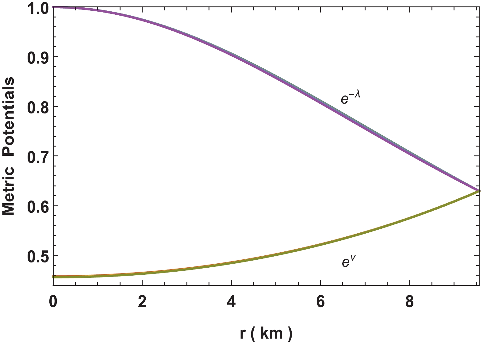
Figure 1. (color online) Variation of metric functions for neutron star in Vela X-1 with parameters
$n = -2$ to$ -18,\; b = 0.001/{\rm{km}}^2,$ $ c = 0.0001, M = 1.77M_\odot$ and$R = 9.56\;{\rm{km}}.$ Using metric potentials given in Eq. (15) and (16), the expressions of
$ \rho, p_r, \Delta $ , and$ p_t $ can be calculated as$ p_r = \frac{f_2(r) \sqrt{a \left[\cosh \left(b r^2+c\right)+1\right]^n}}{8 \pi f_1(r) \left(a r^2 \left(\cosh \left(b r^2+c\right)+1\right)^n+1\right)}, $

(18) $\begin{split} \rho = & \frac{a \left[\cosh \left(b r^2+c\right)+1\right]^{n-1}}{8 \pi \left[a r^2 \left\{\cosh \left(b r^2+c\right)+1\right\}^n+1\right]^2} \\ &\times\Big[a r^2 \left\{\cosh \left(b r^2+c\right)+1\right\}^{n+1} \\ & +2 b n r^2 \sinh \left(b r^2+c\right)+3 \cosh \left(b r^2+c\right)+3\Big], \end{split} $

(19) $\begin{split} \Delta = & \frac{r f_3(r) \sqrt{a r^2 \left[\cosh \left(b r^2+c\right)+1\right]^n} }{f_4(r) \left[\cosh \left(b r^2+c\right)+1\right]} \\& \times {b n \sinh \left(b r^2+c\right)-a \left[\cosh \left(b r^2+c\right)+1\right]^{n+1} \over \left[a r^2 \left\{\cosh \left(b r^2+c\right)+1\right\}^n+1\right]^2}, \\ p_t =& p_r + \frac{\Delta}{8 \pi}. \end{split} $

(20) The variations of pressures, density, anisotropy, equation of state parameters,
$ {\rm d}\rho/{\rm d}r,\; {\rm d}p_r/{\rm d}r $ , and$ {\rm d}p_t/{\rm d}r $ are shown in Figs. 2–6. As values of$ n $ increase the central density, anisotropy, adiabatic index decrease, however, the pressures, equation of state parameters and speed of sounds decrease.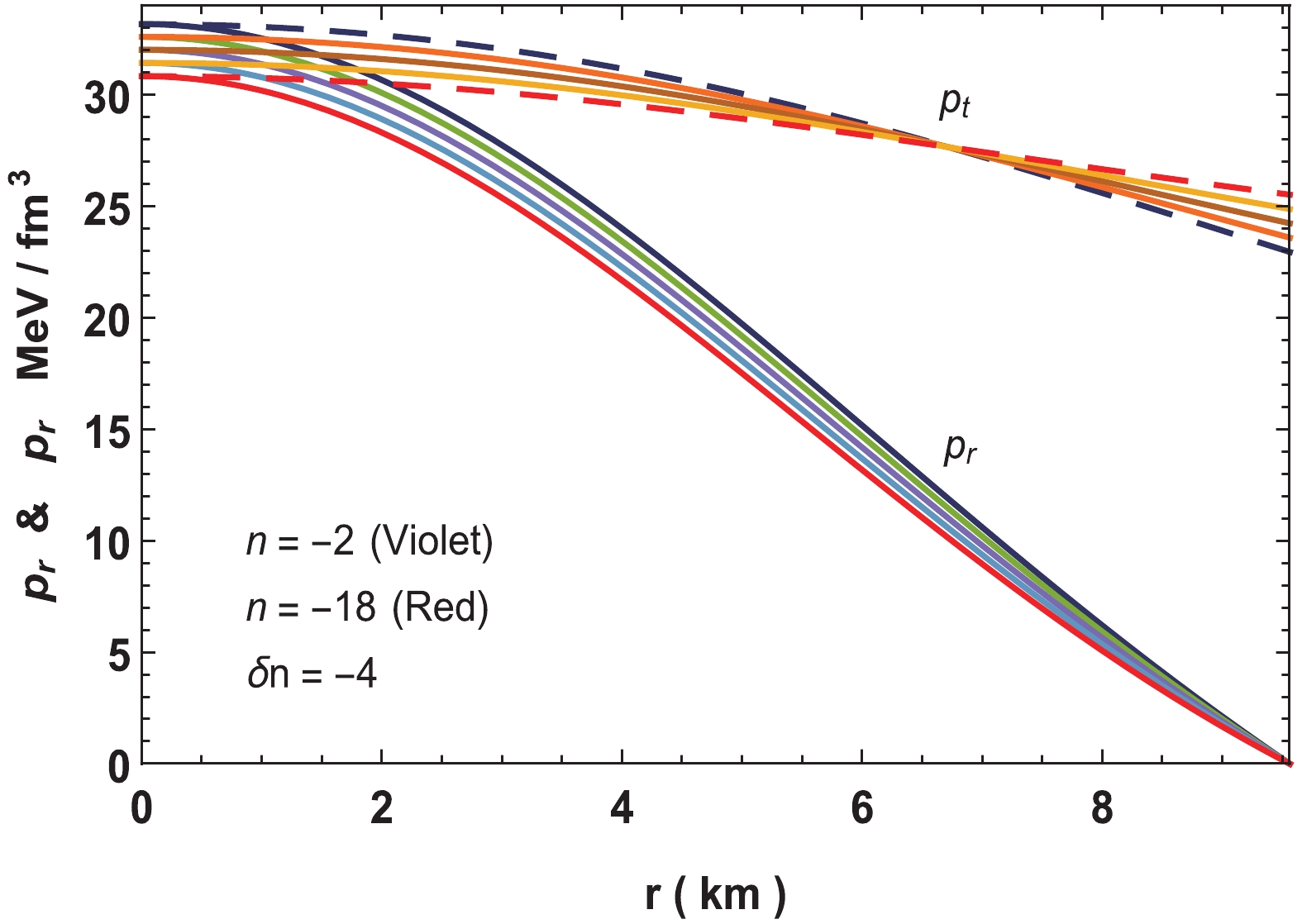
Figure 2. (color online) Variation of pressures for neutron star in Vela X-1 with parameters
$n = -2$ to$ -18,\; b = 0.001/{\rm{km}}^2,$ $ c = 0.0001, M = 1.77M_\odot$ and$R = 9.56\;{\rm{km}}$ . Here,$\delta n$ is the increment in$n$ while ploting the graph.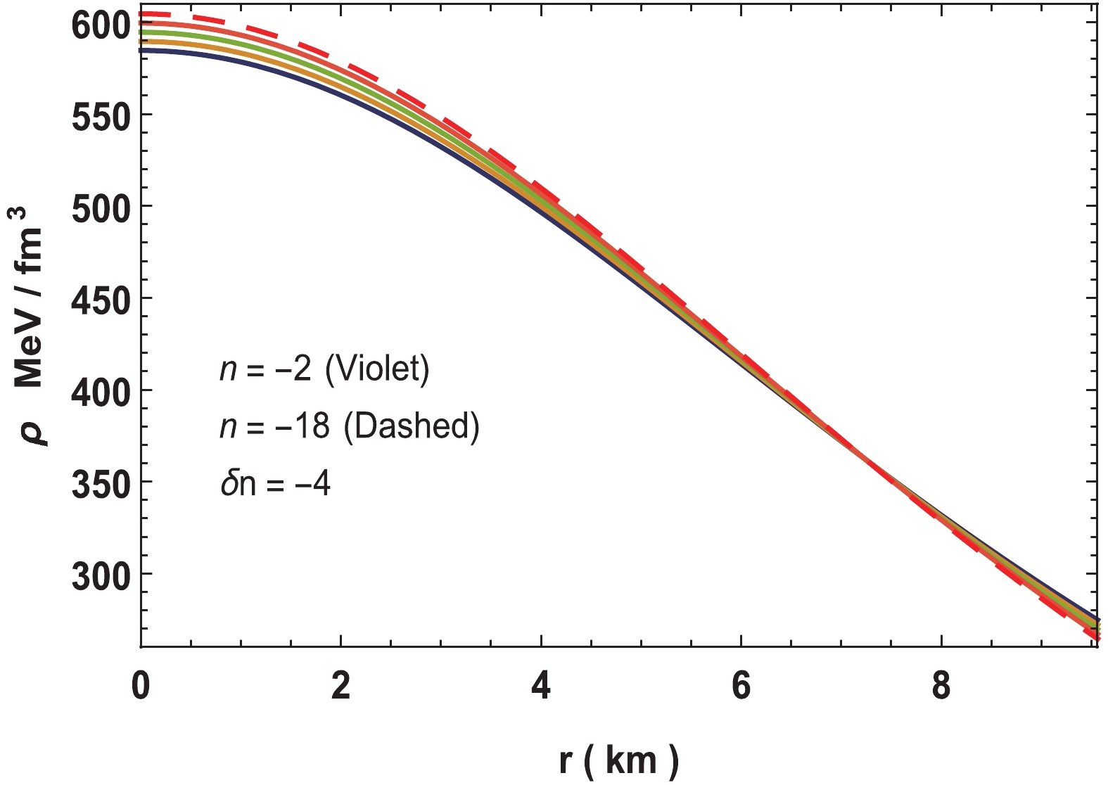
Figure 3. (color online) Variation of density for neutron star in Vela X-1 with parameters
$n = -2$ to$-18,\; b = 0.001/{\rm{km}}^2,$ $\; c = 0.0001, M = 1.77M_\odot$ and$R = 9.56\;{\rm{km}}.$ 
Figure 4. (color online) Variation of pressure anisotropy for neutron star in Vela X-1 with parameters
$n = -2$ to$ -18,\; b = 0.001/{\rm{km}}^2,$ $c = 0.0001, M = 1.77M_\odot$ and$R = 9.56\;{\rm{km}}.$ 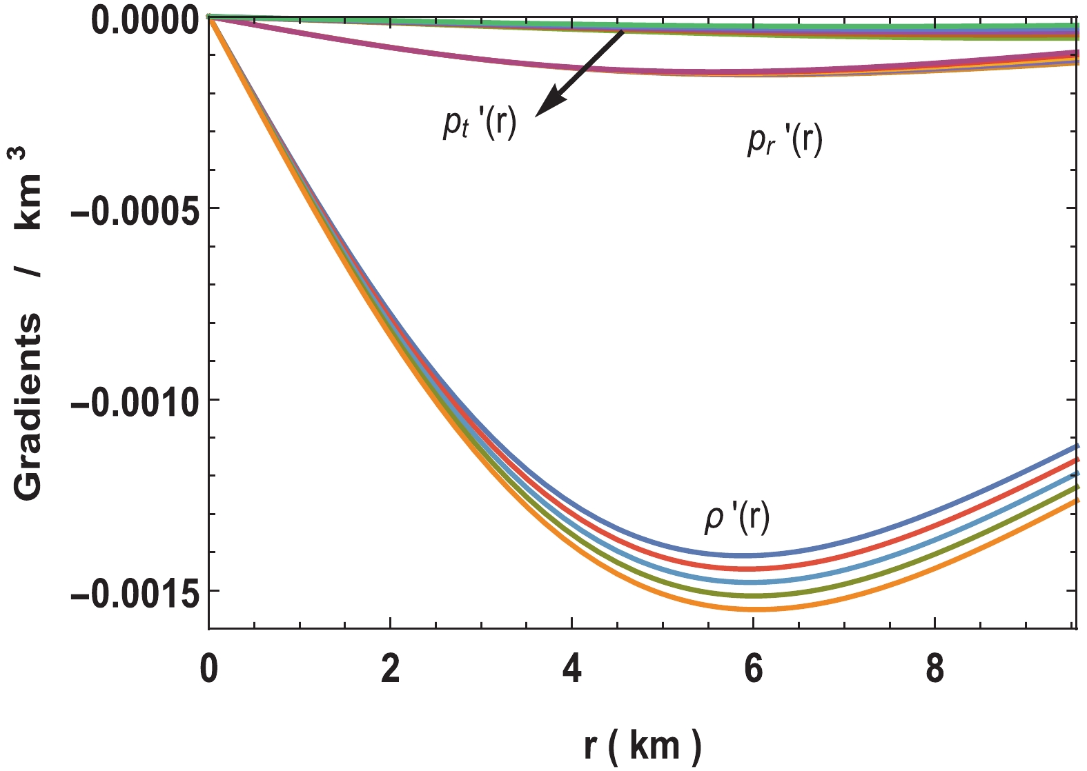
Figure 5. (color online) Variation of pressure and density gradients for neutron star in Vela X-1 with parameters
$n = -2$ to$-18,\; b = 0.001/{\rm{km}}^2,\; c = 0.0001, M = 1.77M_\odot$ and$R = 9.56\;{\rm{km}}.$ 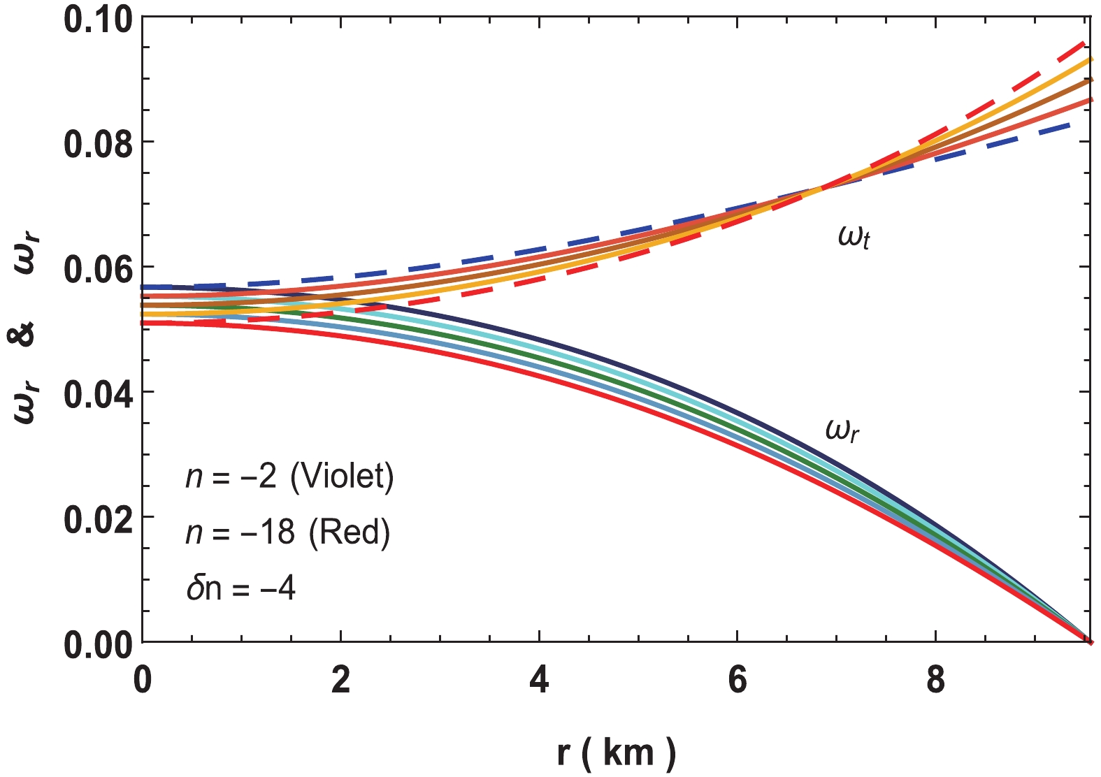
Figure 6. (color online) Variation of equation of state parameters for neutron star in Vela X-1 with parameters
$n = -2$ to$-18,\; b = 0.001/{\rm{km}}^2,\; c = 0.0001, M = 1.77M_\odot$ and$R = 9.56\;{\rm{km}}.$ where,
$\begin{split} f_1(r) =& 2 A b (n+1) r \sqrt{1-\cosh \left(b r^2+c\right)}-\sqrt{2} B \\ &\sinh \left(b r^2+c\right)\sqrt{a r^2 \left[\cosh \left(b r^2+c\right)+1\right]^n} \\ &_2F_1\left[\frac{1}{2},\frac{n+1}{2};\frac{n+3}{2};\cosh ^2\left(\frac{b r^2+c}{2} \right)\right] \\ f_2(r) = & 2 b (n+1) \sqrt{1-\cosh \left(b r^2+c\right)} \Big(2 B r-A\\ &\sqrt{a r^2 \left[\cosh \left(b r^2+c\right)+1\right]^n}\Big) +\sqrt{2} a B r \\ & \sinh \left(b r^2+c\right) \left[\cosh \left(b r^2+c\right)+1\right]^n \, \\ & _2F_1\left[\frac{1}{2},\frac{n+1}{2};\frac{n+3}{2};\cosh ^2\left(\frac{b r^2+c}{2} \right)\right] \\ f_3(r) = & 2 b (n+1) \sqrt{1-\cosh \left(b r^2+c\right)} \Big(B r -A\\ & \sqrt{a r^2 \left[\cosh \left(b r^2+c\right)+1\right]^n}\Big) +\sqrt{2} a B r \end{split} $

$\begin{split} &\sinh \left(b r^2+c\right) \left[\cosh \left(b r^2+c\right)+1\right]^n \,\\ &_2F_1\left[\frac{1}{2},\frac{n+1}{2};\frac{n+3}{2};\cosh ^2\left(\frac{b r^2+c}{2} \right)\right]\\ f_4(r) = & 2 A b (n+1) r \sqrt{1-\cosh \left(b r^2+c\right)} -\sqrt{2} B\\& \sinh \left(b r^2+c\right) \sqrt{a r^2 \left[\cosh \left(b r^2+c\right)+1\right]^n} \, \\ &_2F_1\left[\frac{1}{2},\frac{n+1}{2};\frac{n+3}{2};\cosh ^2\left(\frac{b r^2+c}{2} \right)\right]. \end{split} $

-
Assuming the exterior spacetime to be the Schwarzschild solution, which has to match smoothly with our interior solution and is given by
$ \begin{split} {\rm d}s^2 = \left(1-{2M\over r}\right) {\rm d}t^2-\left(1-{2M\over r}\right)^{-1}{\rm d}r^2 -r^2({\rm d}\theta^2+\sin^2 \theta \; {\rm d}\phi^2). \end{split} $

(21) By matching the first and second fundamental forms the interior solution of Eq. (1) and exterior solution of Eq. (21) at the boundary
$ r = R $ (Darmois-Israel condition [54,55]) we get$\begin{split} {\rm e}^{\nu_b/2} =& 1-{2M \over R} \\=& A-\frac{ f(R) B \sqrt{a {^2} \left[\cosh \left(b R^2+c\right)+1)\right]^n}}{b (n+1)\sqrt{2-2 \cosh \left(b R^2+c\right)}}, \end{split} $

(22) $\begin{split} {\rm e}^{-\lambda_b} = &1-{2M \over R} \\ &= \Bigg[1+ a R^2 \big\{1+ \cosh \left(b R^2+c\right)\big\}^n \Bigg]^{-1}, \end{split} $

(23) $ p_r(R) = 0. $

(24) Using the boundary conditions (22–24), we get
$ a = \frac{2 M \left[\cosh \left(b R^2+c\right)+1\right]^{-n}}{R^2 (R-2 M)} , $

(25) $ A = \frac{B \left[\cosh \left(b R^2+c\right)+1\right]^{-n/2}}{2 \sqrt{a} b (n+1) \sqrt{1-\cosh \left(b R^2+c\right)}}, $

(26) $\begin{split} B = & \frac{\sqrt{a}}{2} \sqrt{1-\frac{2 M}{R}} \Big[\cosh \left(b R^2+c\right)+1\Big]^{n/2} \\ &\times \Bigg[\sqrt{2} a \sinh \left(b R^2+c\right) \left[\cosh \left(b R^2+c\right)+1\right]^n \\ & _2F_1\left[\frac{1}{2},\frac{n+1}{2};\frac{n+3}{2};\cosh ^2\left(\frac{b R^2+c}{2}\right)\right] \\ &+4 b (n+1) \sqrt{1-\cosh \left(b R^2+c\right)} \Bigg]. \end{split} $

(27) -
The central pressure and density at the interior are given by
$ \begin{split} 8\pi p_r(0) = & 8\pi p_t(0) = \Bigg\{\sqrt{2} a B \sinh c \left(\cosh c +1\right)^n \\ & _2F_1\left[\frac{1}{2},\frac{n+1}{2};\frac{n+3}{2};\cosh ^2\left(\frac{c}{2}\right)\right]\Bigg\} \\ &\Bigg\{8 \pi \Big (\sqrt{2} B \sinh c \sqrt{a \left(\cosh c + 1\right)^n}\\ &_2F_1\left[\frac{1}{2},\frac{n+1}{2};\frac{n+3}{2};\cosh ^2\left(\frac{c}{2}\right)\right] \\ &-2 A b (n+1) \sqrt{1-\cosh c}\Big)\Bigg\}^{-1}>0, \end{split} $

(28) $ \rho(0) = \frac{3a \left(\cosh c +1\right)^{n-1} \left(\cosh c + 1\right)}{8\pi}>0. $

(29) The finite central values of the above parameters ensure that the solution is non-singular. The Zeldovich's condition, i.e.,
$ p_r/\rho $ at center is$ \leqslant 1 $ , which is a prerequisite for physical matters. -
The velocity of sound inside the stellar interior can be determined using
$ v_r^2 = {{\rm d}p_r/{\rm d}r \over {\rm d}\rho/{\rm d}r},\; \; \; v_t ^2 = {{\rm d}p_t/{\rm d}r \over {\rm d}\rho/{\rm d}r}. $

(30) For a stable configuration, the stability factor
$ v_t^2-v_r^2 $ should lie between 0 and –1 [56,57]. Variations of sound speed and stability factor are shown in Figs. 7 and 8, respectively. The figures depict that the class of solution satisfy the causality condition and stability criterion. If$ n = 0 $ , some parts of the stability factor becomes positive and hence introduces instability in the model. However, for$ n $ beyond –18, the stability factor seems stable.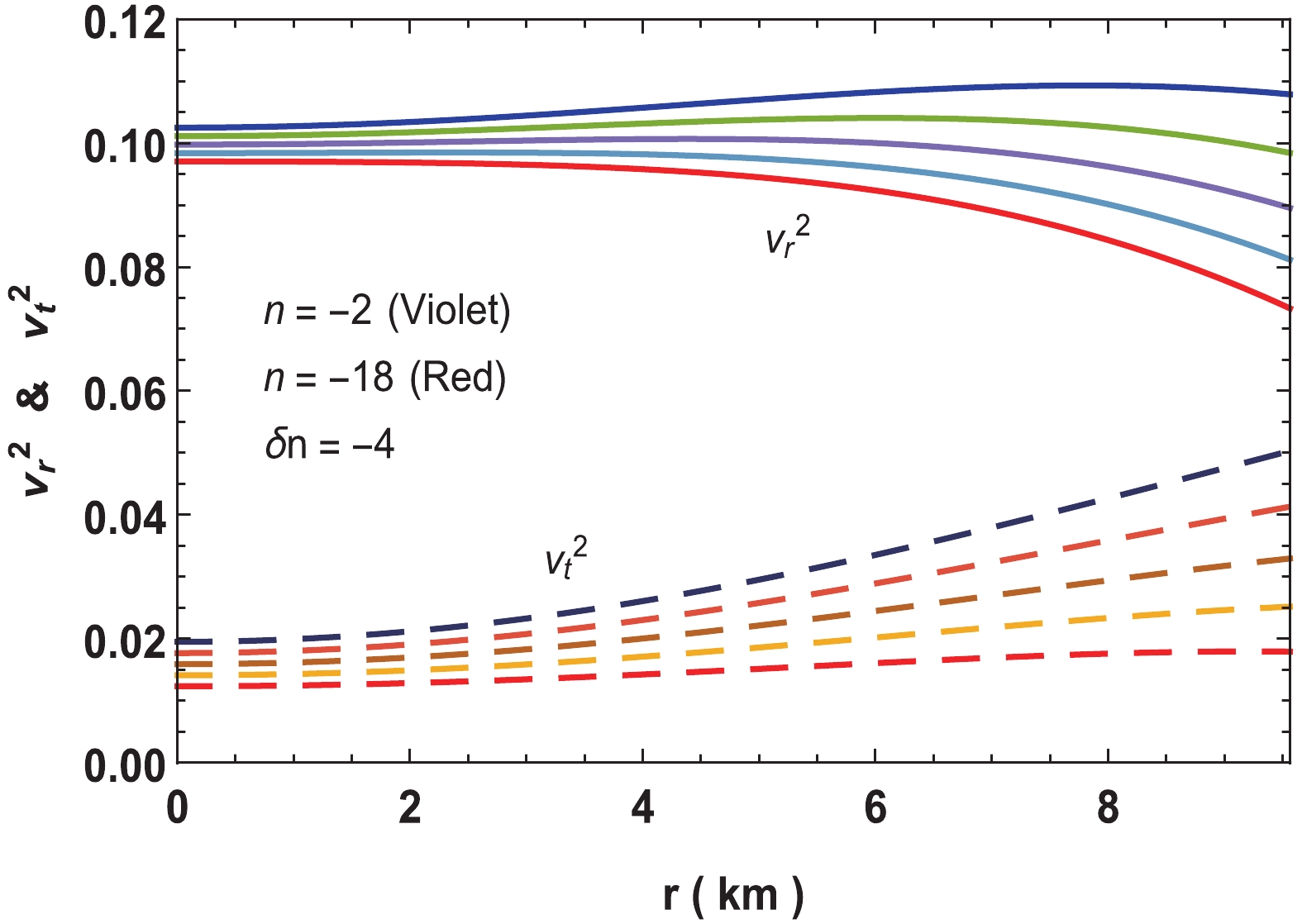
Figure 7. (color online) Variation of velocities of sound for neutron star in Vela X-1 with parameters
$n = -2$ to$-18,\; b = 0.001/{\rm{km}}^2, $ $ c = 0.0001, M = 1.77M_\odot$ and$R = 9.56\;{\rm{km}}.$ 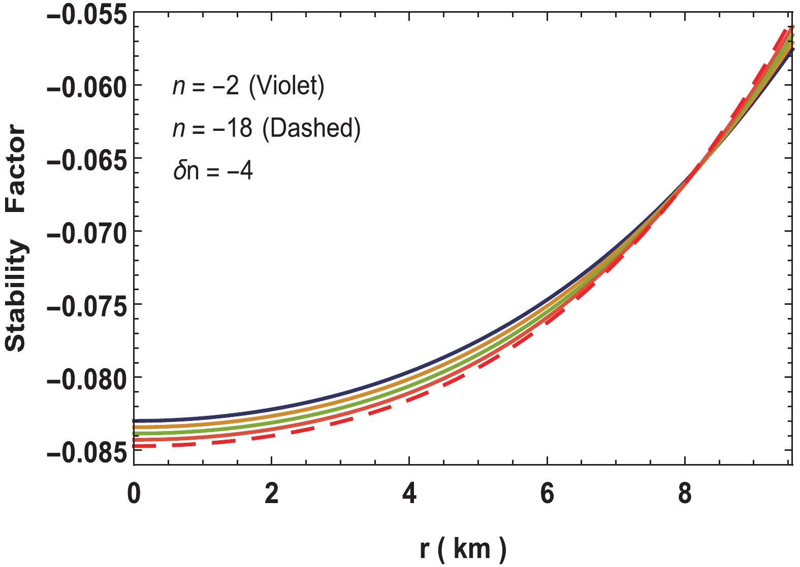
Figure 8. (color online) Variation of stability factor for neutron star in Vela X-1 with parameters
$n = -2$ to$-18,\; b = 0.001/{\rm{km}}^2, $ $ c = 0.0001, M = 1.77M_\odot$ and$R = 9.56\;{\rm{km}}.$ The relativistic adiabatic index is given by
$ \Gamma = {\rho+p_r \over p_r}\; {{\rm d}p_r \over {\rm d}\rho}. $

(31) For a static configuration at equilibrium,
$ \Gamma $ has to be more than 4/3 [58]. Figure 9 shows that the adiabatic index is >4/3.
Figure 9. (color online) Variation of adiabatic index for neutron star in Vela X-1 with parameters
$n = -2$ to$ -18,\; b = 0.001/{\rm{km}}^2,$ $ c = 0.0001, M = 1.77M_\odot$ and$R = 9.56\;{\rm{km}}.$ -
The modified Tolman-Oppenheimer-Volkoff (TOV) equation for anisotropic fluid distribution was given by [59] as
$ -{M_g(\rho+p_r) \over r^2}\; {\rm e}^{(\lambda-\nu)/2}-{{\rm d}p_r \over {\rm d}r}+{2\Delta \over r} = 0, $

(32) provided,
$ M_g(r) = {1\over 2}\; r^2 \nu' {\rm e}^{(\nu-\lambda)/2}. $

(33) The above Eq. (32) can be written in terms of balanced force equation due to anisotropy (
$ F_a $ ), gravity ($ F_g $ ) and hydrostatic ($ F_h $ ), i.e.,$ F_g+F_h+F_a = 0. $

(34) Here
$ F_g = -{M_g(\rho+p_r) \over r^2}\; {\rm e}^{(\lambda-\nu)/2}, $

(35) $ F_h = -{{\rm d}p_r \over {\rm d}r}, $

(36) $ F_a = {2\Delta \over r}. $

(37) The TOV Eq. (34) is plotted in Fig. 10, which shows that all the three forces counter-balance each other. As
$ n $ decreases from –2 to –18, the peak of the$ F_g $ increases,$ F_h $ is almost same from the center up to about 4 km and show significant increment up to the surface. However,$ F_a $ decreases as$ n $ approaches –18.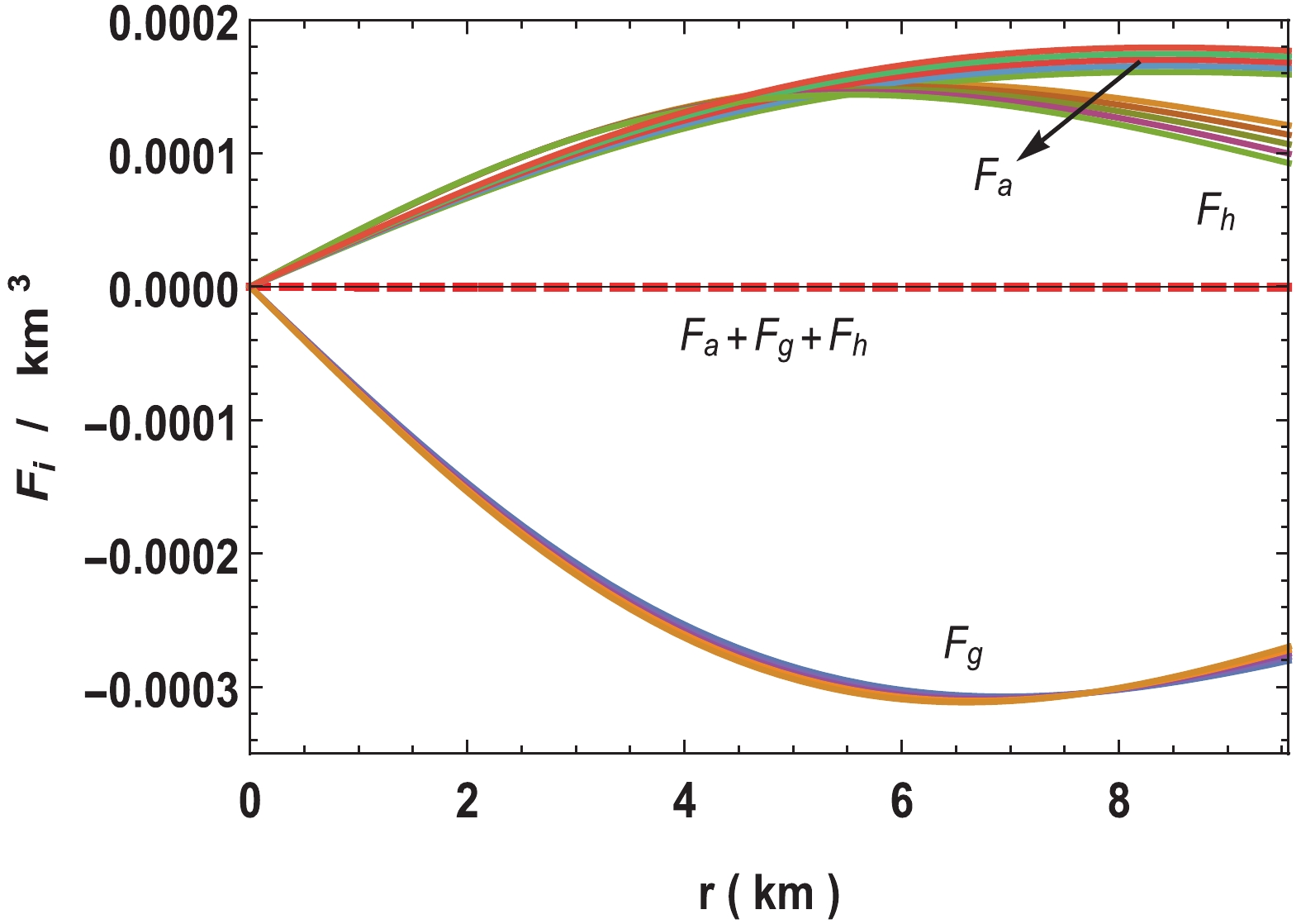
Figure 10. (color online) Variation of forces acting on system via TOV-equation for neutron star in Vela X-1 with parameters
$n = -2$ to$-18,\; b = 0.001/{\rm{km}}^2,\; c = 0.0001, $ $ M = 1.77M_\odot$ and$R = 9.56\;{\rm{km}}.$ -
The satisfaction of the static stability criterion ensures that the solution is static and stable. This was proposed independently by Harrison et al. [60] and Zeldovich-Novikov [61]. According to this criterion, the mass of compact stars must be an increasing function of its central density, i.e.,
$ {\rm d}M/{\rm d}\rho_c >0 $ .For this class of solution, mass as a function of central density can be written as
$ M(\rho_c) = \frac{4 \pi r^3 \rho _c \left[\cosh \left(b R^2+c\right)+1\right]^n}{8 \pi R^2 \rho _c \left[\cosh \left(b R^2+c\right)+1\right]^n+3 (\cosh c+1)^n}, \\ $

(38) $ \begin{split} {\partial M \over \partial \rho_c} =& \frac{12 \pi R^3 \left[\cosh \left(b R^2+c\right)+1\right]^n}{(\cosh c+1)^{-n}} \bigg[3 (\cosh c+1)^n \\& +8 \pi R^2 \rho _c \left\{\cosh \left(b R^2+c\right)+1\right\}^n\bigg]^{-2} >0. \end{split} $

(39) Referring to Fig. 11, we see that the class of solution fulfills this criterion.
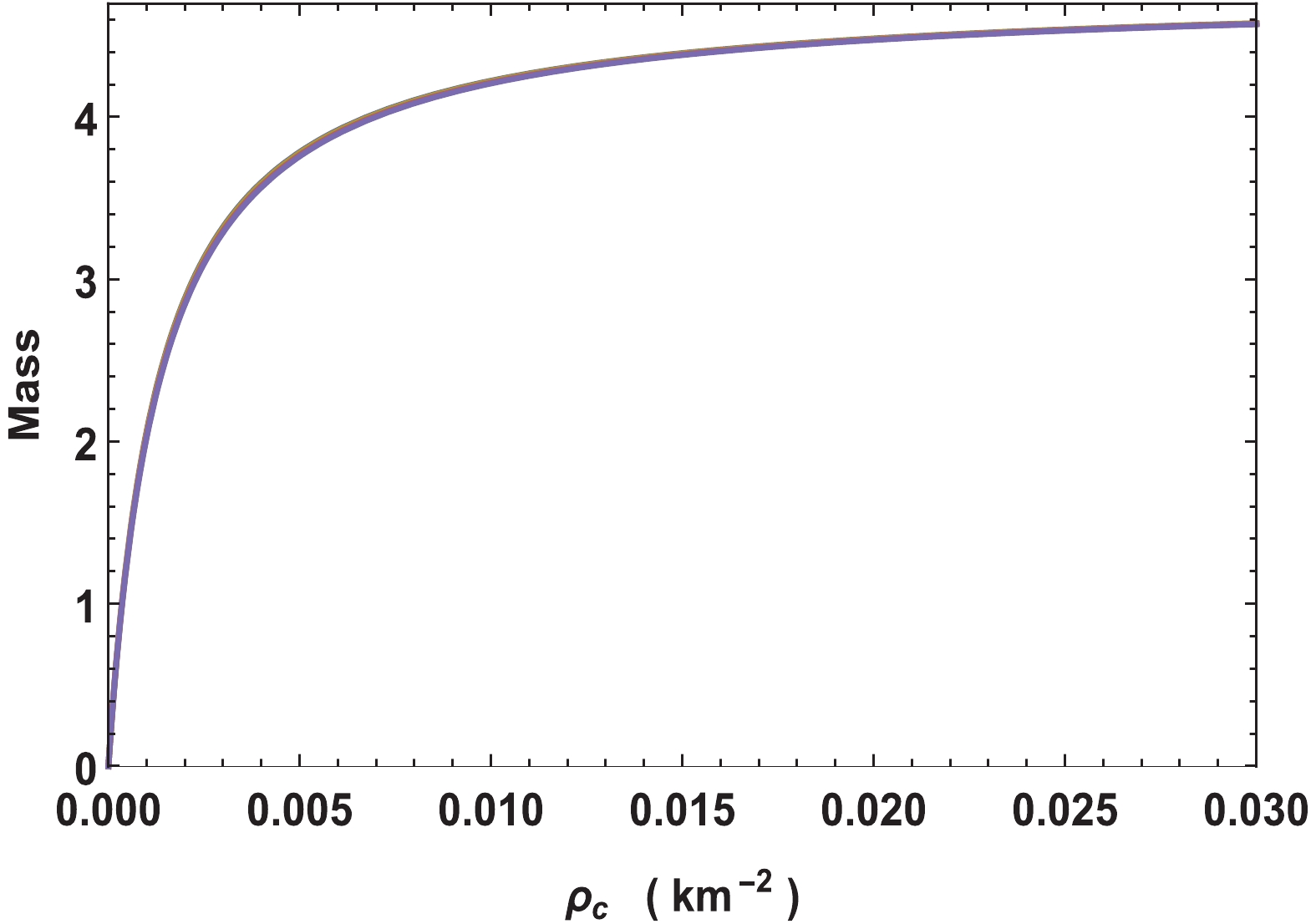
Figure 11. (color online) Variation of mass with central density for neutron star in Vela X-1 with parameters
$n = -2$ to$-18,\; b = 0.001/{\rm{km}}^2$ and$R = 9.56\;{\rm{km}}.$ Now, the gravitational red-shift is given by
$ \begin{split} z (r) = & {\rm e}^{-\nu/2}-1 \\ =& \Bigg[-\frac{ f(r) B \sqrt{a r^2 \left[\cosh \left(b r^2+c\right)+1)\right]^n}}{b (n+1) r \sqrt{2-2 \cosh \left(b r^2+c\right)}}+ A \Bigg]^{-1} - 1. \end{split} $

(40) The variation of red-shift is shown in Fig. 12.
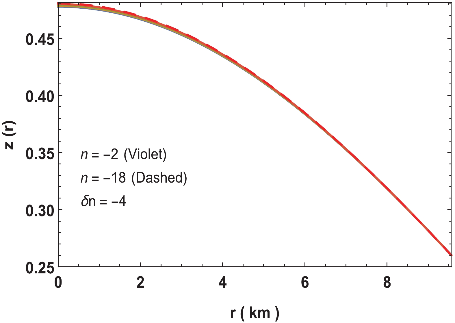
Figure 12. (color online) Variation of red-shift for neutron star in Vela X-1 with parameters
$n = -2$ to -18,$ b = 0.001/{\rm{km}}^2,\; c = 0.0001, $ $ M = 1.77M_\odot$ and$R = 9.56\;{\rm{km}}.$ -
The mass function and compactness factor of the solution can be determined using the equations given below:
$\begin{split} m(r) = & \int_0^r 4\pi\rho(r)\; r^2 \; {\rm d}r \\ =& \frac{a r^3 \left[\cosh \left(b r^2+c\right)+1\right]^n}{2 a r^2 \left[\cosh \left(b r^2+c\right)+1\right]^n+2}, \end{split}$

(41) $ \begin{split} u(r) = & \frac{2 m(r)}{r} \\ =& \frac{a r^2 \left[\cosh \left(b r^2+c\right)+1\right]^n}{a r^2 \left[\cosh \left(b r^2+c\right)+1\right]^n+1}. \end{split} $

(42) The surface red-shift can be found as
$ z_s = {\rm e}^{\lambda_b/2}-1 = (1-u_b)^{-1/2}-1. $

(43) Using the Buchdahl limit, i.e.,
$ u = 8/9 $ , we obtain the maximum surface redshift$ z_s({\rm max}) = 2 $ . When the compactness parameter is zero, the surface red-shift is likewise zero. As the compactness parameter reaches the Buchdahl limit, i.e.,$ u = 8/9 $ , the surface red-shift becomes exactly two. However, if the compactness parameter is beyond the Buchdahl limit, then because of the formation of singularity, the surface red-shift blows up. However, Ivanov [62] has derived that for a realistic anisotropic star models the surface red-shift$ Z_s $ cannot go beyond to 5.211 (this value corresponds to a model without the cosmological constant). -
For a uniformly rotating star with angular velocity
$ \Omega $ , the moment of inertia is given by$ I = {8\pi \over 3} \int_0^R r^4 (\rho+p_r) {\rm e}^{(\lambda-\nu)/2} \; {\omega \over \Omega}\; {\rm d}r $

(44) where the rotational drag
$ \omega $ satisfies the Hartle's equation$ {{\rm d} \over {\rm d}r} \left(r^4 j \; {{\rm d}\omega \over {\rm d}r} \right) = -4r^3\omega\; {{\rm d}j \over {\rm d}r} $

(45) with
$ j = {\rm e}^{-(\lambda+\nu)/2} $ , which has boundary value$ j(R) = 1 $ . The approximate solution of the moment of inertia$ I $ up to the maximum mass$ M_{\rm max} $ is provided by Bejger and Haensel [63] as$ I = {2 \over 5} \Big(1+x\Big) {MR^2}, $

(46) where parameter
$ x = (M/R)\cdot {\rm km}/M_\odot $ . For this class of solution, we plotted the mass vs.$ I $ in Fig. 15 that shows as$ n $ increases, the mass also increases, while the moment of inertia increases up to certain value of mass and subsequently decreases. Comparing Figs. 13 and 15, we see that the mass corresponding to$ I_{\rm max} $ is not equal to$ M_{\rm max} $ from the$ M-R $ diagram. In fact, the mass corresponding to$ I_{\rm max} $ is lower by ~1.46% from the$ M_{\rm max} $ . This happens to the equation of states without any strong high-density softening due to hyperonization or phase transition to an exotic state [64]. Using this graph, we can estimate that the maximum moment of inertia for a particular compact star or by matching the observed$ I $ with the$ I_{\rm max} $ , we can determine the validity of a model. The causality of the maximum mass in Fig. 13, especially the star for$ 2.529M_\odot $ and 12 km is verified from the behaviour of velocity of sound in Fig. 14.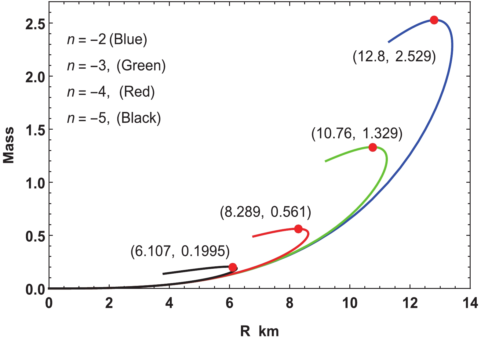
Figure 13. (color online) Variation of mass with radius for
$a = 0.01, \; b = 0.001$ and$c = 0.0001.$ 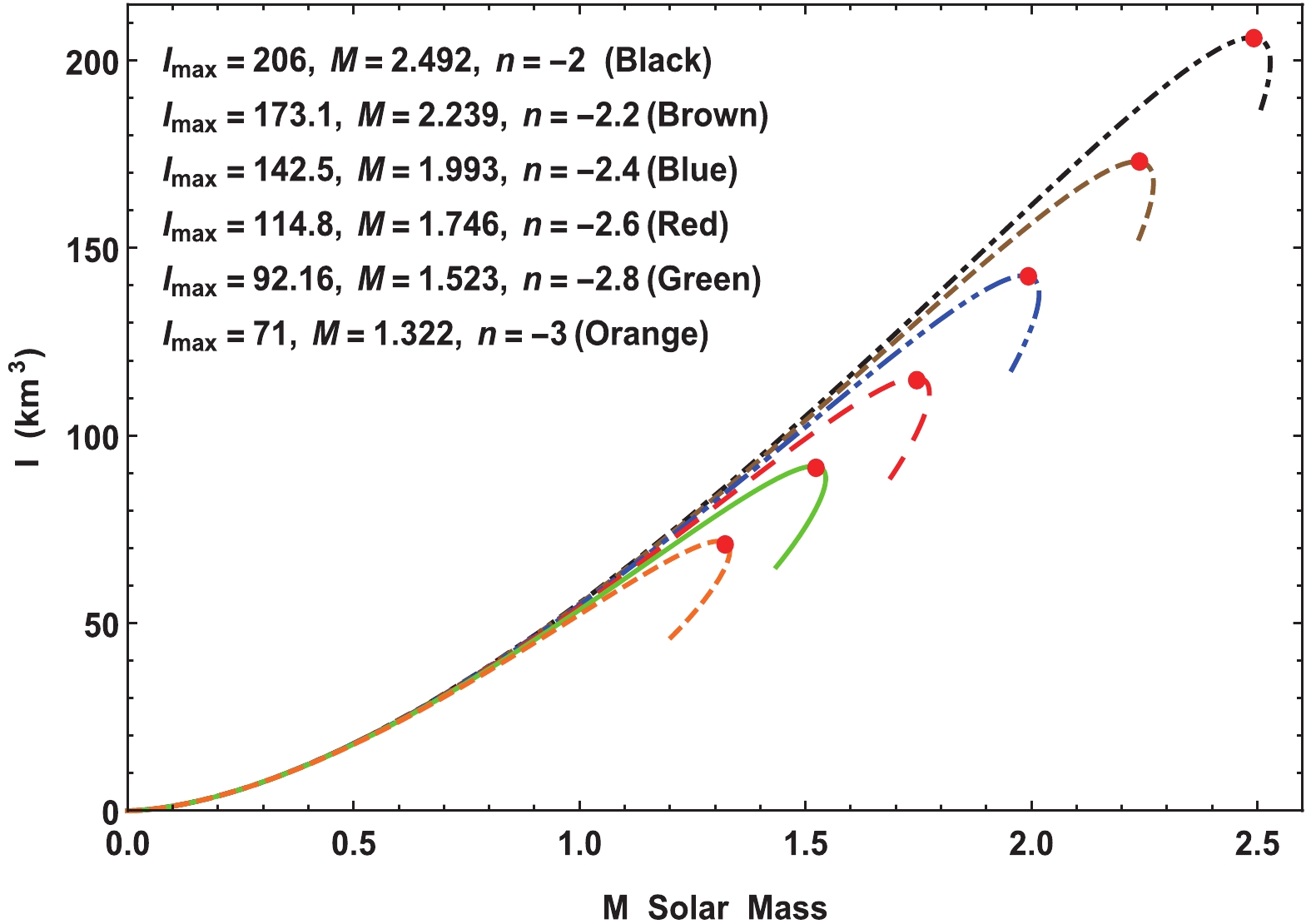
Figure 15. (color online) Variation of moment of inertia with mass for
$n = -2$ to$n = -3$ taking$a = 0.01 /{\rm{km}}^2,\; $ $ b = 0.001/{\rm{km}}^2,\; c = 0.0001.$ 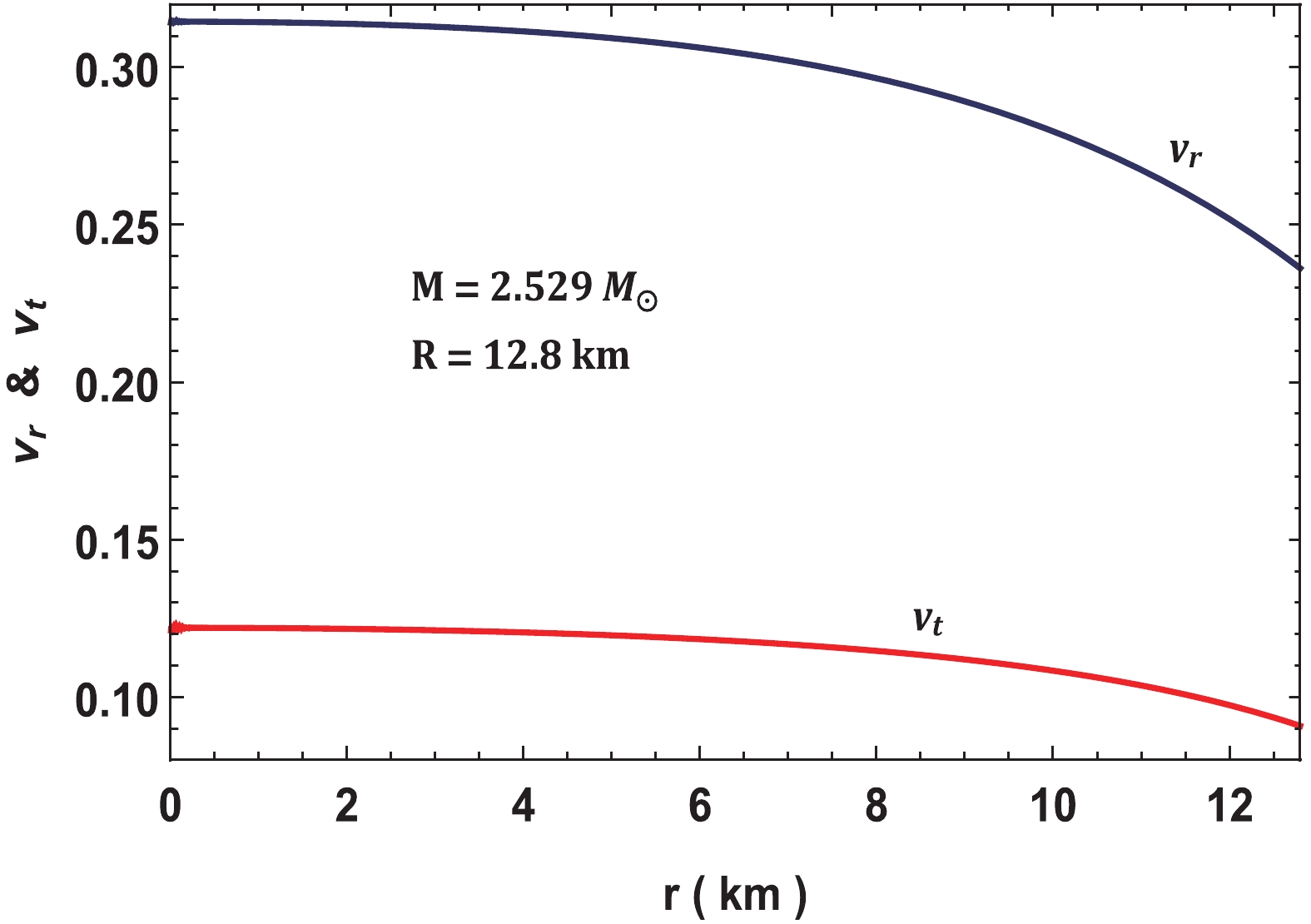
Figure 14. (color online) Variation of velocity of sound for
$2.529M_\odot$ and 12.8 km.A rotating compact star can hold higher
$ M_{\rm max} $ than a non-rotating one. The mass relationship between a non-rotating and rotating compact star is given in the units ($ G = C = 1 $ ) and can be written as [65]$ M_{\rm rot} = M_{\rm non-rot}+{1 \over 2}I\Omega^2. $

(47) Because of the centrifugal force, the radius at the equator increases up to some factor as compared to the static one. Cheng and Harko [66] found the approximate radii for static and rotating stars as
$ R_{\rm rot}/R_{\rm non-rot} \approx 1.626 $ , respectively. Assuming the compact star is rotating in the Kepler frequency$ \Omega_K = (GM_{\rm non-rot}/R^3_{\rm non-rot})^{1/2} $ and using the Cheng-Harko formula, we plotted the$ M-R $ graph for rotating and non-rotating stars (Fig. 16). The corresponding frequency of a rotating star can be determined as [67]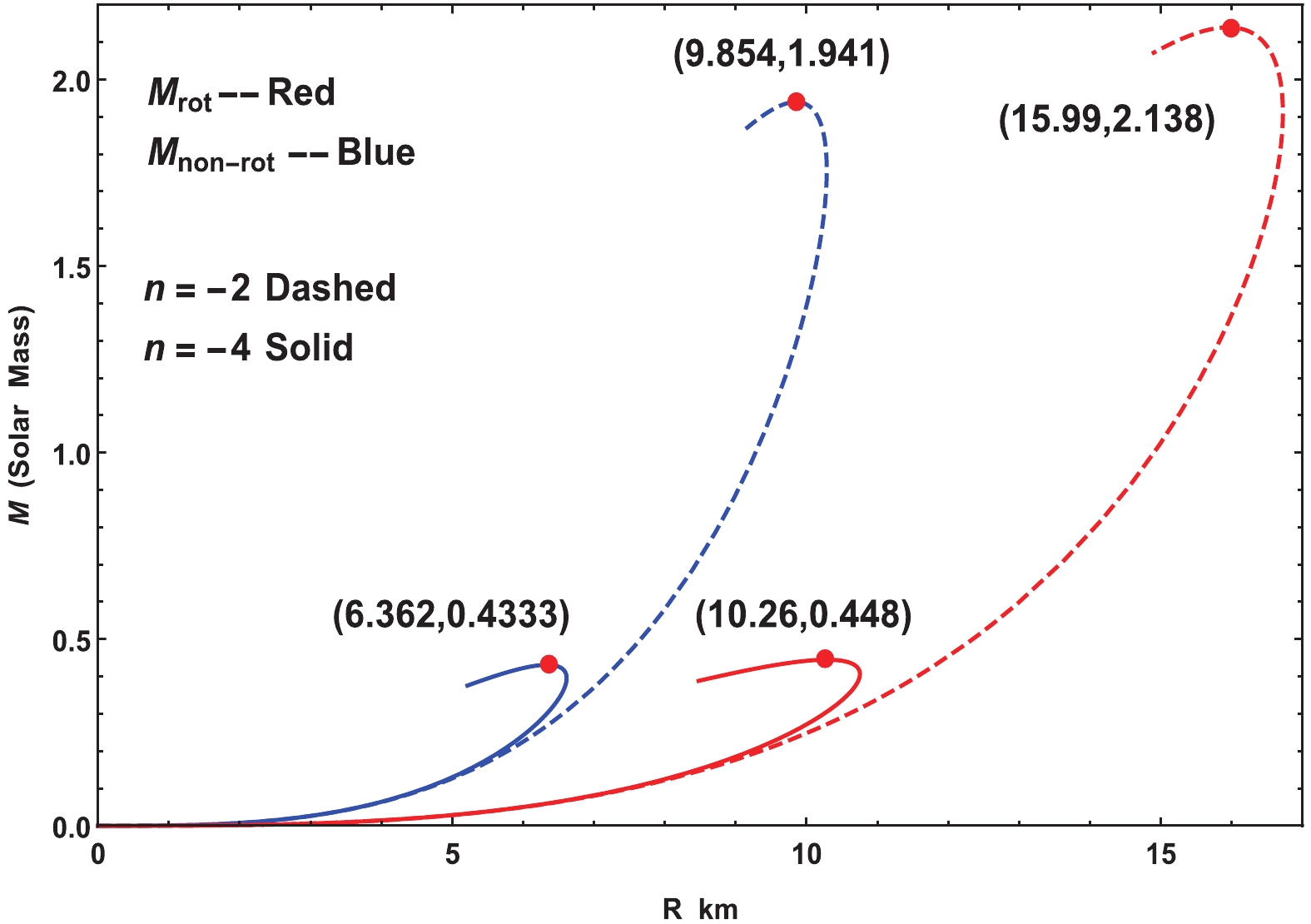
Figure 16. (color online) Variation of mass with radius for
$n = -2$ &$n = -4$ taking$a = 0.01 /{\rm{km}}^2,\; b = 0.001/{\rm{km}}^2,\; c = 0.0001$ for a rotating and non-rotating star.$ \nu \approx 1.22 \left({R_{\rm non-rot} \over 10 {\rm km}}\right)^{-3/2} \left({M_{\rm non-rot} \over M_\odot}\right)^{1/2}\; {\rm kHz}. $

(48) The variation of frequency with mass is shown in Fig. 17. This shows that the frequency of rotation corresponds to the maximum mass. In contrast, we like to mention that recently, the direct detection of the gravitational wave (GW) signal
$ {\rm GW}1- 70817 $ has been reported by the LIGO-Virgo collaboration from a binary compact star system [68]. New constraints for the tidal deformability of the 1.4 solar mass compact stars ($ \Lambda_{1.4} $ ) have been estimated as$ \Lambda_{1.4} < 800 $ [69], which can also place constraints on the equation of state (EOS) for the star matter and constrain the parameter sets for phenomenological models. In the studies of Refs. [69–71], researchers have used different phenomenological models to calculate the properties of the tidal deformability and the maximum mass of neutron stars or quark stars with the constraints of$ {\rm GW}1- 70817 $ , which can provide other alternative methods to constrain the parameter sets in the models.
Figure 17. (color online) Variation of rotational frequency with mass for
$n = -2$ to$n = -3$ taking$a = 0.01 /{\rm{km}}^2,\; $ $ b = 0.001/{\rm{km}}^2,\; c = 0.0001$ for a rotating and non-rotating star. -
Any physical solutions other than those representing exotic matters must fulfill all the energy conditions, i.e., strong, weak, null, and dominant energy conditions, which are stated as follows,
$ {\rm{NEC}} \;\;:\;\; T_{\mu \nu}l^\mu l^\nu \geqslant 0\; {\rm{or}}\; \rho+p_i \geqslant 0 \quad\quad\quad\quad\quad\quad $

(49) $ {\rm{WEC}} \;\;:\;\; T_{\mu \nu}t^\mu t^\nu \geqslant 0\; {\rm{or}}\; \rho \geqslant 0,\; \rho+p_i \geqslant 0 \quad\quad\quad $

(50) $ \begin{array}{l} {\rm{SEC}} \;\;:\;\; T_{\mu \nu}t^\mu t^\nu - \dfrac{1}{ 2} T^\lambda_\lambda t^\sigma t_\sigma \geqslant 0 \; {\rm{or}}\; \rho+\displaystyle\sum_i p_i \geqslant 0. \\ {\rm{DEC}} \;\;:\;\; T_{\mu \nu}t^\mu t^\nu \geqslant 0 \; {\rm{or}}\; \rho \geqslant |p_i| \\ \quad\quad\quad\;\;\;\;{\rm{where}}\; T^{\mu \nu}t_\mu \in {\rm{nonspace-like \;vector}}. \end{array} $

(51) where
$ i\equiv ({\rm radial}\; r,\; {\rm transverse} \; t),\; t^\mu $ and$ l^\mu $ are the time-like vector and null vector, respectively.Because the pressure and density are positive throughout the stellar objects, it is obvious that the energy conditions NEC, WEC, and SEC are satisfied vacuously. We have shown the graphical representation for dominant energy conditions in Figs. 18-20, where it can be observed that our solutions are also valid under dominant energy conditions.
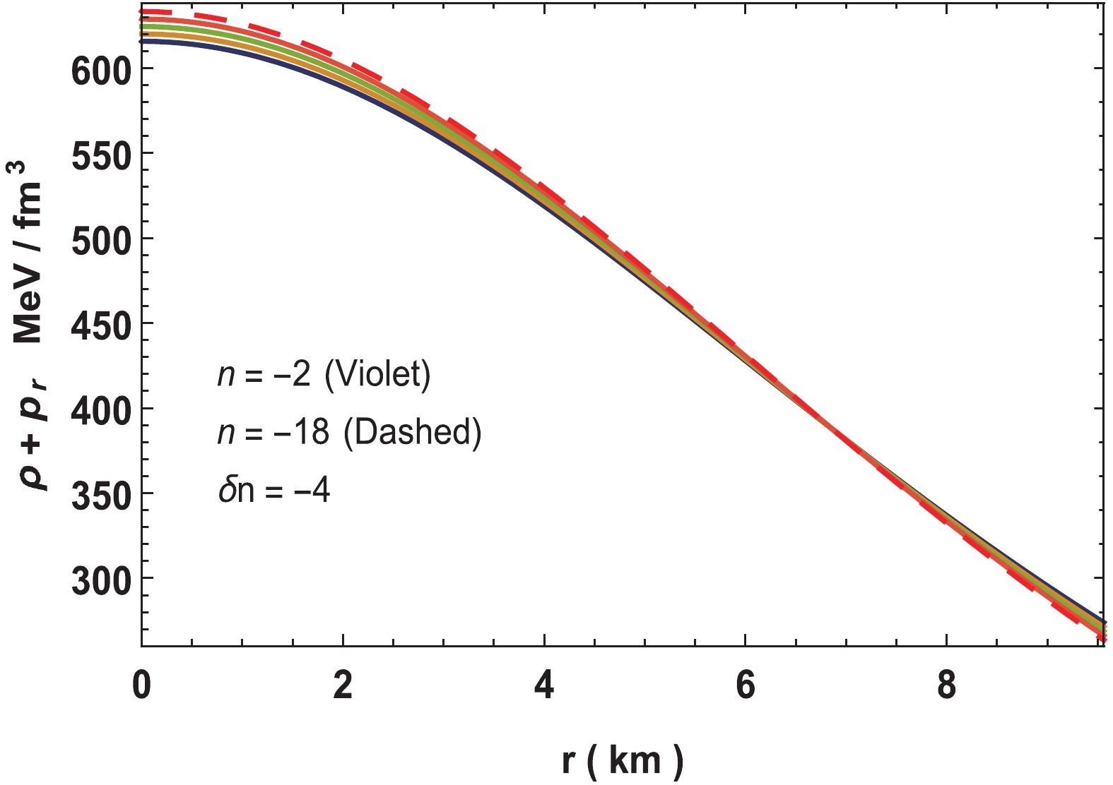
Figure 18. (color online) Variation of
$\rho +p_r$ for neutron star in Vela X-1 with parameters$n = -2$ to$-18,\; b = 0.001/{\rm{km}}^2, \; $ $c = 0.0001,\;M = 1.77M_\odot$ and$R = 9.56\;{\rm{km}}.$ 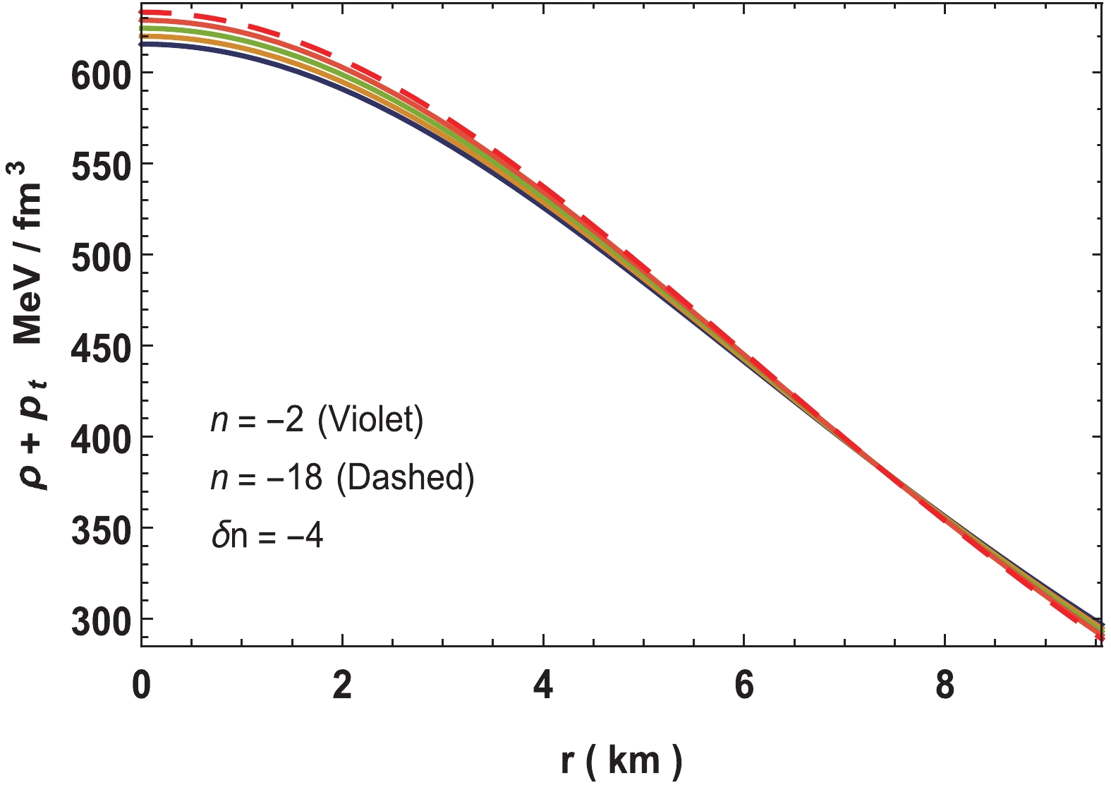
Figure 19. (color online) Variation of
$\rho +p_t$ for neutron star in Vela X-1 with parameters$n = -2$ to$-18,\; b = 0.001/{\rm{km}}^2, \;$ $c = 0.0001,\; M = 1.77M_\odot$ and$R = 9.56\;{\rm{km}}.$ 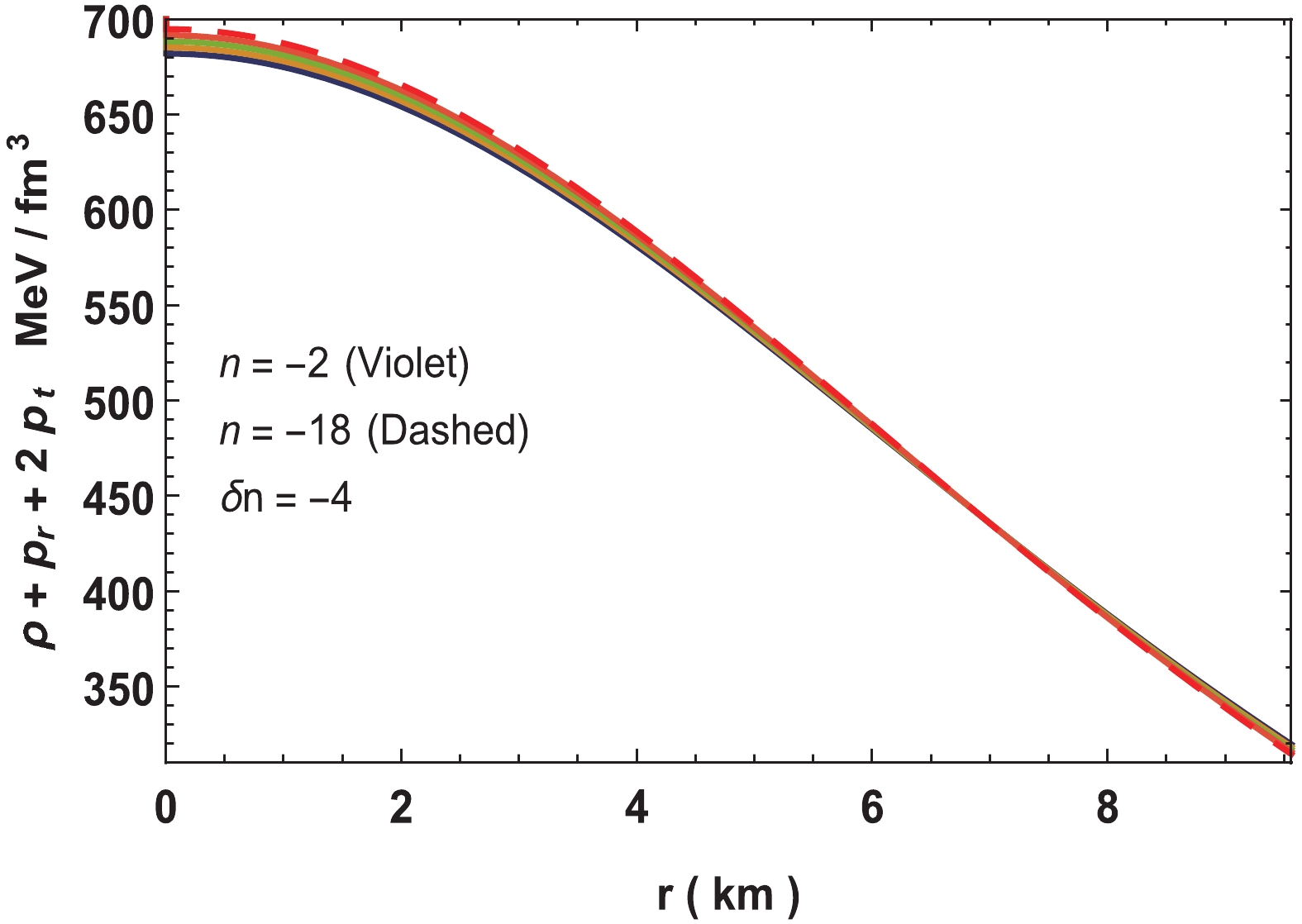
Figure 20. (color online) Variation of
$\rho +p_r+2p_t$ for neutron star in Vela X-1 with parameters$n = -2$ to$ -18,\; b = 0.001/{\rm{km}}^2,$ $c = 0.0001, M = 1.77M_\odot$ and$R = 9.56\;{\rm{km}}.$ n $ a $ 

$ A $ 

$ B $ 

$M \; M_\odot$ 

$ R\;{\rm{ km}}$ 

$ z_c $ 

$ \rho_c \times 10^{14} $ 

$ g/cc $ 

$ \rho_s\times 10^{14} $ 

$ g/cc $ 

$ p_c\times 10^{34} $ 

$ {\rm dyne}/{\rm cm}^2 $ 

$ \Gamma_{rc} $ 

−2 0.0259 0.6766 0.03183 1.77 9.56 0.477 10.44 4.89 5.31 1.91 −6 0.4170 0.6763 0.03183 1.77 9.56 0.478 10.50 4.85 5.22 1.93 −10 6.7279 0.6759 0.03183 1.77 9.56 0.479 10.59 4.81 5.13 1.95 −14 108.55 0.6756 0.03183 1.77 9.56 0.480 10.68 4.76 5.04 1.98 −18 1751.4 0.6753 0.03183 1.77 9.56 0.481 10.77 4.71 4.94 2.00 Table 1. Central and surface values of some parameters for different values of
$ n .$ -
A new family of non-singular solutions of the Einstein field equations for compact stars under embedding class one condition is presented. The thermodynamical quantities for stellar matter like anisotropic pressures, baryon density, red-shift, and the velocity of sound have been investigated using the Karmarkar condition of embedding class one spacetime.
Based on various physical analyses, such as the equilibrium condition (TOV-equation), static stability criterion (
$ \partial M/\partial \rho_c > 0 $ ), Bondi condition ($ \Gamma_r > 4/3 $ ), singularity free ($ \rho_c,\; p_{rc} = p_{tc}>0 $ ), Zeldovich condition ($ p_{rc}/\rho_c < 1 $ ) and satisfaction of energy conditions, imply that the new family of solutions is possible to represent realistic matter. Therefore, these solutions are suitable to model physical compact stars.For
$ n = 0 $ , some parts of the stability factor becomes positive, resulting in instability of the model. However, beyond$ n = -18 $ , the stability factor is stable. From Fig. 10, one can observe that as$ n $ decreases from –2 to –18, the peak of the$ F_g $ increases,$ F_h $ is almost same from the center up to about 4 km and shows significant increment till the surface. However,$ F_a $ decreases as$ n $ approaches –18. Using the Buchdahl limit, we obtain the maximum surface red-shift$ z_s({\rm max}) = 2 $ . For a zero value of the compactness parameter, the surface red-shift is likewise zero. As the compactness parameter reaches the Buchdahl limit, the surface red-shift becomes exactly two. However, if the compactness parameter is beyond the Buchdahl limit, then because of the formation of singularity the surface red-shift blows up. The unique character of these solutions can be observed from the fact that for a large range of parameter$ n $ , the profiles of density, pressures, equation of state parameters, and speed of sounds seem to be different, however, the profiles of the adiabatic index, mass with central density, and red-shift are not very different. This indicates that for modeling compacts, various choices of the equation of state (EoS) can be made for a single compact star. These choices of EoS lead to various structures of interior space-times, however, physical properties like mass, radius, luminosity etc., look the same to an external observer. Fig. 13 shows that smaller values of parameter$ n $ lead to smaller$ M_{\rm max} $ and$ R_{\rm max} $ . From Fig. 13, we can see that for$ n = -2 $ the values of ($ M_{\rm max},\; R_{\rm max} $ ) are (12.8 km, 2.529$ M_\odot $ ), which is under the theoretical limit proposed by Rhoades and Ruffini [72], while for$ n = -5 $ , the values are 6.107 km and 0.1995$ M_\odot $ . However, in recent studies, heavy pulsars such as PSR J1614-2230, PSR J0348+0432, and MSR J0740+6620 were discovered [73–75], which has set the new record of the maximum mass of the pulsars. Further, from Fig. 7, it is also clear that the values of$ v_r^2 $ and$ v_t^2 $ are at their maximum for$ n = -2 $ . Therefore, we conclude that the stiffness of the equation of state decreases as$ n $ decreases. The sensitivity to EoS is sharper in the$ M-I $ graph than$ M-R $ , because the peak points in these graphs are sharper in the former graph than the latter. After the complete analysis of solutions with various mathematical and graphical representations, we conclude that the solution is physically reasonable. With the inclusion of a small rotation, we also showed that the maximum mass that can be held by the system increases, and the corresponding radius likewise increases due to the centrifugal force. Larger values of$ n $ yield higher$ M_{\rm max} $ . The corresponding frequency of rotation can also be determined using the Haensel et al. formula [67]. In Table 1, we have shown different physical quantities and their corresponding parameters for n=-2 to n=-18. -
Herrera et al. [76] proposed an algorithm for generating all types of spherically symmetric static solutions using two physical quantities, namely anisotropy and a function related to the redshift. These two generators are respectively defined as
$ \zeta(r) = {\nu'\over 2} +{1 \over r} \; \; \; {\rm{and}} \; \; \; \Pi(r) = 8\pi(p_r - p_t). $

(52) For this solution, they are found to be
$\begin{split} \zeta(r) = & {1 \over r}+4 b B (n+1) r^2 \sinh ^2\left[\frac{1}{2} \left(b r^2+c\right)\right] \\ &\sqrt{a \left(\cosh \left(b r^2+c\right)+1\right)^n} \Bigg[B \sinh \left(b r^2+c\right) \\ & \sqrt{2-2 \cosh \left(b r^2+c\right)} \sqrt{a r^2 \left(\cosh \left(b r^2+c\right)+1\right)^n} \\ & _2F_1\left[\frac{1}{2},\frac{n+1}{2};\frac{n+3}{2};\cosh ^2\left(\frac{1}{2} \left\{b r^2+c\right\}\right)\right] \\ & +4 A b (n+1) r \sinh ^2\left(\frac{1}{2} \left\{b r^2+c\right\}\right) \Bigg]^{-1},\end{split} $

(53) $ \Pi(r) = -\Delta (r). \quad\quad\quad\quad\quad\quad\quad\quad\quad\quad\quad\quad\quad\quad\quad\quad\quad\;\;\;$

(54) S.K. Maurya acknowledges to the administration of the University of Nizwa for their continuous support and encouragement.
Static fluid spheres admitting Karmarkar condition
- Received Date: 2019-07-22
- Accepted Date: 2019-12-06
- Available Online: 2020-03-01
Abstract: We explore a new relativistic anisotropic solution of the Einstein field equations for compact stars based on embedding class one condition. For this purpose, we use the embedding class one methodology by employing the Karmarkar condition. Employing this methodology, we obtain a particular differential equation that connects both the gravitational potentials


 DownLoad: