


 Abstract
 HTML
HTML Reference
 Related
 PDF
PDF


-
Black holes are solutions of Einstein equation in general gravitational theories, and the black hole is one of the fascinating parts of our universe. Black holes are thermal systems because they were found to have temperature and entropy. The temperature of a black hole is proportional to the surface gravity at the event horizon. In the case of general relativity, the entropy, known as Bekenstein–Hawking entropy, is usually proportional to the area of the event horizon in the framework of black hole thermodynamics [1-6]. It is noticed that beyond general relativity, the entropy is not simply proportional to the surface area of the horizon and additional terms would appear, see for example [7-9]. However, when one considers quantum fields in the vicinity of black holes, the area law of entropy will get additional quantum corrections. Till now, physicists have made several attempts to disclose the microscopic essence of black hole entropy and its connection with the area of event horizon. For instance, the authors of [10-12] computed the entropy by evaluating the Euclidean action. The relationship between the entropy and instanton amplitude, which describes the pair production of charged black holes, can be seen in [13]. The proposal that the entropy is the Noether charge of the bifurcate Killing horizon has been addressed in [14, 15]. Later, the symmetry-based approach to black hole entropy was proposed, which connects the central charge of the conformal field theory to the black hole entropy [16, 17]. This proposal of the central charge of the Virasoro algebra on the horizon was generalized in the case of Witt algebra [18], surface charge algebra [19], Virasoro algebra null surfaces [20], and 2−cocycles on the Lie algebra [21].
We know that the consideration of quantum mechanics gives rise to thermal Hawking radiation, which does not carry information. One viewpoint is that the quantum gravity theory, such as string theory and loop quantum gravity, is required to understand this information loss paradox. However, it was addressed in [22] that the interior of black holes has a ‘fuzzball’ structure. This gives a qualitative picture of how a classical idea breaks down in black hole physics and the information paradox can be resolved. In particular, the authors somehow took care of both the near horizon behaviors and the possible existence of singularity instead of focusing on one of them in the discussion. It is noticed that the microscopic derivation of black hole entropy was proposed with the D-brane method in string theory [23] and the brick wall model [24]. However, the entanglement entropy is a measure of the correlation between subsystems, which are separated by a boundary called the entangling surface. It is a measure of information loss due to the division of the system; therefore, it depends on the geometry of the boundary [25, 26]. The entanglement entropy model, as one of the most attractive candidates of the black hole entropy, has been widely studied [27-34].
In this paper, we aim to investigate the entropy of a massive BTZ black hole [35, 36] via calculating its entanglement entropy by introducing a massless quantum scalar field. We shall apply the discretized approach to evaluate the entropy of the quantum scalar field in space-time by analyzing a similar harmonic oscillator, and we closely follow the procedure shown in [25, 37, 38]. We note that, similar studies on (rotating) a BTZ black hole with a massless or massive scalar field have been performed in [39, 40], where the authors numerically analyzed the effect of angle momentum
$ (J) $ and mass of scalar field$ (m_s) $ on the coefficients in the entanglement entropy of the BTZ black hole.Here, we shall focus on the effect of the mass of graviton on the entanglement entropy in a three-dimensional massive black hole. As is known, black holes provide a particle environment for testing gravity and are incredibly important theoretical tools for exploring general gravity, and the Schwarzschild black hole is the most general spherically symmetric vacuum solution. Massive gravity theory is one of the theories beyond Einstein's gravity theory with massless graviton. In recent years, some cosmologists have proposed the idea of a massive graviton to modify general relativity. One can also make contributions to explain the accelerated expansion of the universe without dark energy [41]. Early attempts at constructing in massive gravity have been established, such as linear theory of gravity [42] and nonlinear model for massive gravity [43]. Recently, significant progress has been made in constructing massive gravity theories, which would prevent instability [44-50]. Various phenomenologies of massive gravity have also been investigated widely. Moreover, the massive terms in the gravitational action break the diffeomorphism symmetry in the bulk, which corresponds to momentum dissipation in the dual boundary field theory [51].
This paper is organized as follows. We briefly review the massive BTZ black hole in three-dimensional gravity theory in Section 2. We study the formula of the entanglement entropy of the massless quantum scalar field, and then evaluate the (sub-)leading coefficients of the entropy by fitting the numerical results in Section 3. Section 4 concludes the study.
-
We first briefly review the three-dimensional Einstein massive gravity with the action [35, 36]
$ {\cal J} = -\frac{1}{16\pi }\int {\rm d}^{3}x\sqrt{-g}\left[ {\cal R}-2\Lambda+m^{2}\sum\limits_{i}^{}c_{i}{\cal U}_{i}(g,f)\right] , $

(1) where
$ {\cal R} $ is the scalar curvature,$ \Lambda = -1/L^2 $ is the cosmological constant, and the last terms are Fierz–Pauli mass terms where m denotes the mass of graviton [52]. Here,$ c_{i} $ is a constant and$ {\cal U}_{i} $ represents the symmetric polynomials of the eigenvalues of the$ 3\times 3 $ matrix$ {\cal K}_{\nu }^{\mu }\equiv\sqrt{g^{\mu \alpha }f_{\alpha \nu }} $ . In this matrix, g denotes the background metric, and the fixed rank−2 symmetric tensor f is the reference metric, which is inevitably included to construct the massive term of the graviton in massive gravity, and its form will be chosen later. As addressed in [45, 53],$ {\cal U}_{i} $ can be written as$ \begin{array}{l} {\mathcal U}_{1} = \left[ {\cal K}\right] ,\;\;\;\;\;{\cal U}_{2} = \left[ {\cal K}\right] ^{2}-\left[ {\cal K}^{2}\right] ,\\ {\cal U}_{3} = \left[ {\cal K}\right] ^{3}-3\left[ {\cal K}\right] \left[ {\cal K}^{2}\right] +2\left[ {\cal K}^{3}\right] , \\ {\cal U}_{4} = \left[ {\cal K}\right] ^{4}-6\left[ {\cal K}^{2} \right] \left[ {\cal K}\right] ^{2}\!+\!8\left[ {\cal K}^{3}\right] \left[ {\cal K}\right] +3\left[ {\cal K}^{2}\right] ^{2}\!-\!6\left[ {\cal K} ^{4}\right],\cdots \end{array} $

(2) where the dots denote the higher-order terms of
$ {\cal K} $ . The square root in$ {\cal K} $ denotes the matrix square root, i.e,$ (\sqrt{{\cal K}})^{\mu}_{\nu}(\sqrt{{\cal K}})^{\nu}_{\kappa} = {\cal K}^{\mu}_{\; \; \kappa} $ , and the rectangular brackets denote traces, i.e.,$ [{\cal K}]={\cal K}^{\mu}_{\mu} $ and$ [{\cal K}^2]=({\cal K}^2)^{\mu}_{\; \; \mu} $ with$({\cal K}^2)_{\mu\nu}= $ $ {\cal K}_{\mu\alpha}{\cal K}^{\alpha}_{\; \; \nu} $ . We note that the study of ghost-free massive gravity can be seen in [46, 48].Action (1) gives us the Einstein equation
$ G_{\mu \nu }+\Lambda g_{\mu \nu }+m^{2}\chi _{\mu \nu } = 0, $

(3) where the Einstein tensor
$ G_{\mu \nu } $ and massive term$ \chi _{\mu \nu } $ are$ G_{\mu \nu }= R_{\mu \nu }-\frac{1}{2}g_{\mu \nu }R, $

(4) $\begin{split} {\chi _{\mu \nu }} = & - \frac{{{c_1}}}{2}\left( {{{\cal U}_1}{g_{\mu \nu }} - {{\cal K}_{\mu \nu }}} \right) - \frac{{{c_2}}}{2}\left( {{{\cal U}_2}{g_{\mu \nu }} - 2{{\cal U}_1}{{\cal K}_{\mu \nu }} + 2{\cal K}_{\mu \nu }^2} \right) \hfill \\ & - \frac{{{c_3}}}{2}({{\cal U}_3}{g_{\mu \nu }} - 3{{\cal U}_2}{{\cal K}_{\mu \nu }} + 6{{\cal U}_1}{\cal K}_{\mu \nu }^2 - 6{\cal K}_{\mu \nu }^3) - \frac{{{c_4}}}{2}({{\cal U}_4}{g_{\mu \nu }} \hfill \\ &- 4{{\cal U}_3}{{\cal K}_{\mu \nu }} + 12{{\cal U}_2}{\cal K}_{\mu \nu }^2 - 24{{\cal U}_1}{\cal K}_{\mu \nu }^3 + 24{\cal K}_{\mu \nu }^4) \hfill {\text{.}}\\ \end{split} $

(5) In order to solve the equation of motion, we take the ansatz of the metric as
$ {\rm d}s^{2} = -f(r){\rm d}t^{2}+f^{-1}(r){\rm d}r^{2}+r^{2}{\rm d}\varphi ^{2}, $

(6) where
$ f(r) $ is an arbitrary function of radial coordinate, and we will work with$ L = 1 $ such that$ \Lambda = -1 $ . Also, following [54], we choose the ansatz of the reference metric as$ f_{\mu \nu } = \partial_{\mu}\phi^a\partial_{\nu}\phi^b\eta_{ab} = {\rm diag}(0,0,c^{2}), $

(7) where c is a positive constant,
$ \phi^a(x) $ is coordinate transformation using$ \eta_{ab} $ , and different choices for the$ \phi^a $ fields correspond to different gauges. Then, with the metric ansatz (7),$ {\cal U}_{i} $ in (2) can be calculated as [46, 55]$ {\cal U}_{1} = \frac{c}{r},\;\;\;\;\;{\cal U}_{2} = {\cal U}_{3} = {\cal U}_{4} = \cdots = 0, $

(8) which means that in a three-dimensional case, the only contribution of massive terms comes from the term
$ {\cal U}_{1} $ in the action. In principle, the choice of the reference metric could be arbitrary [48], however, here we follow [54] to choose the form (7). As is addressed in [54], with this choice, the graviton mass term preserves general covariance in the t and r coordinates, but breaks it in spatial coordinates. Then only one field$ \phi^{\varphi} $ is needed due to the spatial reference metric, so that the bulk could be seen to fill with homogeneous solid. Moreover, this makes us manage to find the analytical solution of the black hole.Subsequently, the independent Einstein equations are
$ rf^{\prime }(r)-2r^{2} -m^{2}cc_{1}r = 0, $

(9) $ \frac{r^{2}}{2}f^{\prime \prime }(r)-r^{2} = 0,$

(10) the solution to which is
$ f(r) = r^{2}-M +m^{2}cc_{1}r. $

(11) Here, M is an integration constant, which is related to the total mass of the black hole. We note that in the absence of a massive term with
$ m = 0 $ , the solution recovers neutral BTZ black hole$ f\left( r\right) = r^{2}-M $ without rotation.Applying the standard method, we obtain the temperature of the black hole as
$ T = \frac{ r_{+}}{2\pi }+\frac{m^{2}cc_{1}}{ 4\pi }, $

(12) where
$ r_{+} $ is the event horizon satisfying$ f(r_+) = 0 $ and the Hawking entropy of the black hole is$ S = \frac{\pi }{2}r_{+}. $

(13) For the convenience of further study, we perform transformation of the metric. The solutions to
$ f(r) = 0 $ are$ r_{\pm} = \frac{-m^{2}cc_{1}\pm\sqrt{m^{4}c^{2}c_{1}^{2}+4M}}{2}. $

(14) Then, we introduce the proper length,
$ \rho $ , by the coordinate transformation$ r^{2} = r^{2}_{+}\cosh^2\rho+r^{2}_{-}\sinh^{2}\rho. $

(15) Subsequently, the metric of the black hole can be rewritten in terms of the proper length as
$ {\rm d}s^{2} = -u^{2}{\rm d}t^{2}+{\rm d}\rho^{2}+\frac{[m^{2}+\sqrt{m^{4}+4(M+u^{2})}]^{2}}{4}{\rm d}\varphi^{2} $

(16) where we have defined
$ u^{2} = r^{2}-M+m^{2}cc_{1}r $ . In the following study, we will set$ c = c_1 = 1 $ without loss of generality. -
The action of a massless scalar field in the curved space-time is
$ S_{\rm scalar} = -\frac{1}{2}\int {\rm d}^3x\sqrt{-g}g^{\mu\nu}\partial_{\mu}\Phi\partial_{\nu}\Phi. $

(17) In the background of massive BTZ black hole (16), considering the cylindrical symmetry of the system and the form of the scalar field
$ \Phi(t,\rho, \varphi) = \sum\limits_{n}\Phi_{n}(t,\rho){\rm e}^{{\rm i}n\varphi}, $

(18) we then further evaluate action (17) as
$ \begin{split} {S_{\rm scalar}} = &- \frac{1}{2}\int {{{\rm d}^3}} x\sum\limits_n \left( - \frac{{{m^2} + \sqrt {{m^4} + 4(M + {u^2})} }}{{2u}}\dot \Phi _n^2 \right.\hfill \\ &+ \frac{{u[{m^2} + \sqrt {{m^4} + 4(M + {u^2})} ]}}{2}{({\partial _\rho }{\Phi _n})^2} \hfill \\ &{ \left.+ {n^2}\frac{{2u}}{{{m^2} + \sqrt {{m^4} + 4(M + {u^2})} }}\Phi _n^2\right) = \int {{{\rm d}^3}} x\sum\limits_n {\cal L}_n ,} \end{split}$

(19) where we define
$ {\cal L}_n $ as the Lagrangian density for the$ n- $ mode.The conjugate momentum corresponding to
$ \Phi_{n} $ is given by$ \pi_{n} = \frac{\delta{\cal L}_n}{\delta \dot\Phi_n} = \frac{2un^{2}}{m^{2}+\sqrt{m^{4}+4(M+u^{2})}}\Phi_{n}. $

(20) Therefore, the Hamiltonian density of the system is
$\begin{split} H =& \sum\limits_n {{H_n}} = \sum\limits_n {\left( {\frac{1}{2}\int {\rm d} \rho \pi _n^2(\rho )} \right.} \hfill \\ & \left. { + \frac{1}{2}\int {\rm d} \rho {\rm d}\rho '{\psi _n}(\rho ){V_n}(\rho ,\rho '){\psi _n}(\rho ')} \right) \hfill \\ \end{split} $

(21) where we introduced
$ \psi_{n}(t,\rho) = \sqrt{\frac{2u}{m^{2}+\sqrt{m^{4}+4(M+u^{2})}}}\Phi_{n}(t,\rho) $

(22) and
$ \begin{split} {\psi _n}(\rho ){V_n}(\rho ,\rho '){\psi _n}(\rho ') =& \frac{{u[{m^2} + \sqrt {{m^4} + 4(M + {u^2})} ]}}{2} \hfill \\ & \times{\left({\partial _\rho }\left(\sqrt {\frac{{2u}}{{{m^2} + \sqrt {{m^4} + 4(M + {u^2})} }}} \right){\psi _n}\right)^2} \hfill \\ & { + \frac{{2u{n^2}}}{{{{\left({m^2} + \sqrt {{m^4} + 4(M + {u^2})} \right)}^2}}}\psi _n^2.} \end{split}$

(23) To proceed, we discretize the system for the convenience of computation via
$ \rho \rightarrow (A-1/2)a, \qquad \delta(\rho-\rho') \rightarrow\delta_{AB}/a, $

(24) where A, B = 1, 2 ... N and "a" is the UV cut-off length, such that
$ N\propto r_+/a $ . We note that the continue limit recovers when$ a\rightarrow 0 $ and$ N\rightarrow \infty $ as the size of the system is fixed. Then, the Hamiltonian of the discretized system can be obtained by replacing$\begin{split} \psi_{n}(\rho) \rightarrow q^{A}, \quad \pi_{n}(\rho) \rightarrow p_{A}/a, \quad V(\rho,\rho') \rightarrow V_{AB}/a^{2} \end{split} $

(25) in (21), the expression of which is then
$ H_D = \sum\limits_{A,B = 1}^N\left(\frac{1}{2a}\delta^{AB}p_{nA}p_{nB}+\frac{1}{2}V_{AB}^{n}q_n^A q_n^B\right). $

(26) Here,
$ V_{AB}^{n} $ is$ N\times N $ matrix representation is given as$ \begin{array}{l} (V_{AB}^{(n)}) = \begin{bmatrix} \Sigma_{1}^{(n)} & \Delta_{1} & & & & \\ \Delta_{1} & \Sigma_{2}^{(n)} & \Delta_{2} & & & \\ & \ddots & \ddots & \ddots & & \\ & & \Delta_{A-1} & \Sigma_{A}^{(n)} & \Delta_{A} & & \\ & & & \ddots &\ddots &\ddots \\ \end{bmatrix} , \end{array} $

(27) with
$ \begin{split} \Sigma _A^{(n)} = &\frac{{2{u_A}}}{{{m^2} + \sqrt {{m^4} + 4(M + u_A^2)} }} \\ & \times\left(\frac{{{u_{A + 1/2}}\Big[{m^2} + \sqrt {{m^4} + 4(M + u_{A + 1/2}^2)}\;\Big]}}{2} \right. \\ &\left.- \frac{{{u_{A - 1/2}}\Big[{m^2} + \sqrt {{m^4} + 4(M + u_{A - 1/2}^2)}\; \Big]}}{2}\right) \\ & + {n^2}\frac{{4{u^2}}}{{{{\Big[{m^2} + \sqrt {{m^4} + 4(M + u_A^2)}\; \Big]}^2}}} \end{split}$

(28) and
$\begin{split} {\Delta _A} = &- \frac{{{u_{A + 1/2}}\Big[{m^2} + \sqrt {{m^4} + 4(M + u_{A + 1/2}^2)}\; \Big]}}{2} \hfill \\ & \times \sqrt {\frac{{2{u_{A + 1}}}}{{{m^2} + \sqrt {{m^4} + 4(M + u_A^2)} }}} \hfill \\ & { \times \sqrt {\frac{{2{u_A}}}{{{m^2} + \sqrt {{m^4} + 4(M + u_{A + 1/2}^2)} }}} .} \end{split} $

(29) After determining the Hamiltonian (26)–(29), we apply the method shown in Appendix A to evaluate the entanglement entropy of the system.
-
Following Appendix A, the entanglement entropy of the above system is given by [56]
$ S = \lim\limits_{N\to\infty}S(n_{B},N) = S_{0}+2\sum\limits_{n = 1}^{\infty}S_{n}, $

(30) where
$ S(n_{B},N) $ is the entanglement entropy of the total system N with partition$ n_{B} $ ;$ S_{0} $ is the entanglement entropy of the system for$ n = 0 $ and$ S_{n} $ is the entropy of the subsystem for a given "n", respectively.We first study the entanglement entropy of the massive BTZ black hole at a large N, which means that the change of result is not significant with increasing N. The numerical results are shown in Table 1. We numerically calculate
$ S_n $ for$ n_B = 10,50 $ , and$ 100 $ at fixed$ N = 100 $ , and then perform summation over "n" as$ S_{\rm total} $ . In particular, we show the results with different masses of graviton. The properties are summarized as follows. First, for fixed N and m, a larger$ n_B $ corresponds to higher$ S_n $ and$ S_{\rm total} $ . Second, with fixed$ n_B $ and m,$ S_n $ decreases for a larger n and finally it becomes slightly significant to the total entanglement entropy. These properties are similar to those observed in [39]. Third, with fixed$ n_B $ ,$ S_{\rm total} $ is suppressed by stronger mass of graviton.$ n_B $ 

$ S_0 $ 

$ S_1 $ 

$ S_2 $ 

$ \cdots $ 

$ S_{\rm total} =S $ 

m = 0 m = 0.5 m = 1 m = 0 m = 0.5 m = 1 m = 0 m = 0.5 m = 1 $\cdots$ 

m = 0 m = 0.5 m = 1 10 0.98177 0.98190 0.98145 0.00732 0.00548 0.00331 0.00010 0.00046 0.00027 $\cdots$ 

0.99795 0.99399 0.98875 50 1.70383 1.70259 1.68877 0.25020 0.18895 0.15193 0.02178 0.01702 0.013599 $\cdots$ 

2.25842 2.12277 2.02639 100 2.39708 2.38928 2.33553 0.79353 0.72815 0.67098 0.14988 0.12739 0.156145 $\cdots$ 

4.35903 4.16412 4.06405 Table 1. The effect of mass of graviton on the entanglement entropy with fixed
$N = 100$ for different$n_B$ .Next, we numerically evaluate the entanglement entropy of the system with finite N. The entropy of the massive BTZ black hole is proportional to the area of the horizon, as shown in (13), which we rewrite as
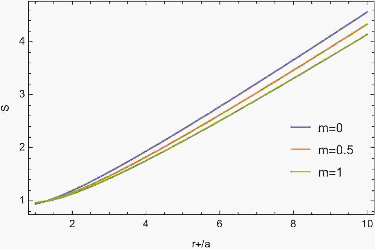
$S = c_1 r_+/a$ , and$c_1$ is a constant while a is the UV cut-off used to discretize the system. Considering the quantum effect, we should estimate the logarithmic correction to the black hole entropy as①$ S_q = c_1 r_+/a+c_2\log(r_+/a)+c_3 , $

(31) where
$c_1, c_2$ , and$c_3$ are the coefficients to be determined. We numerically calculate the entropy (30) and fit the results by (31), as shown in Fig. 1. The fitted coefficients affected by the mass of graviton are shown in Table 2. We see that the coefficient of the linear term,$c_1$ , decreases as m, which is further fitted in Fig. 2.$c_1$ in the entanglement entropy is dependent of m, which is different from the constant in the Hawking entropy (13). This is reasonable because, as we mentioned in footnote 3, that whether this entanglement entropy is exactly the black hole entropy is still an open question. It is worthwhile to point out that the entanglement entropy of a massive black hole has also been holographically studied in [57, 58] via the Ryu–Takayanagi formula [59], and it was found that the massive of graviton would affect the entanglement entropy. Therefore, we argue that the massive term has explicit print on the entanglement entropy of black hole could be a universal property in massive gravity, even though deep physics calls for further study. Our result shows that the effect of mass of graviton on the entropy is similar to that of mass of scalar field observed in [40]. The sub-leading coefficient,$c_2$ is negatives and also decreases as the mass increases while the fitting of$c_3$ is positive and bigger in a massive BTZ black hole.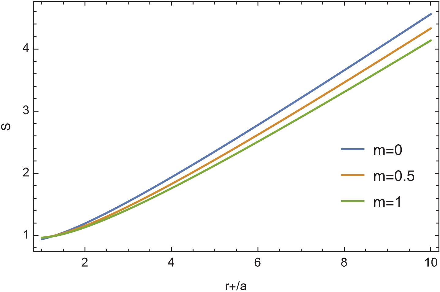
Figure 1. (color online) Entropy fitted by logarithmic correction (31) for different masses of graviton.
c $m=0$ 

$m=0.5$ 

$m=1 $ 

$c_1$ 

0.489594 0.480959 0.461284 $c_2$ 

−0.34156 −0.417998 −0.425697 $c_3$ 

0.452134 0.484263 0.504732 Table 2. Coefficients in (31) by fitting the entropy.
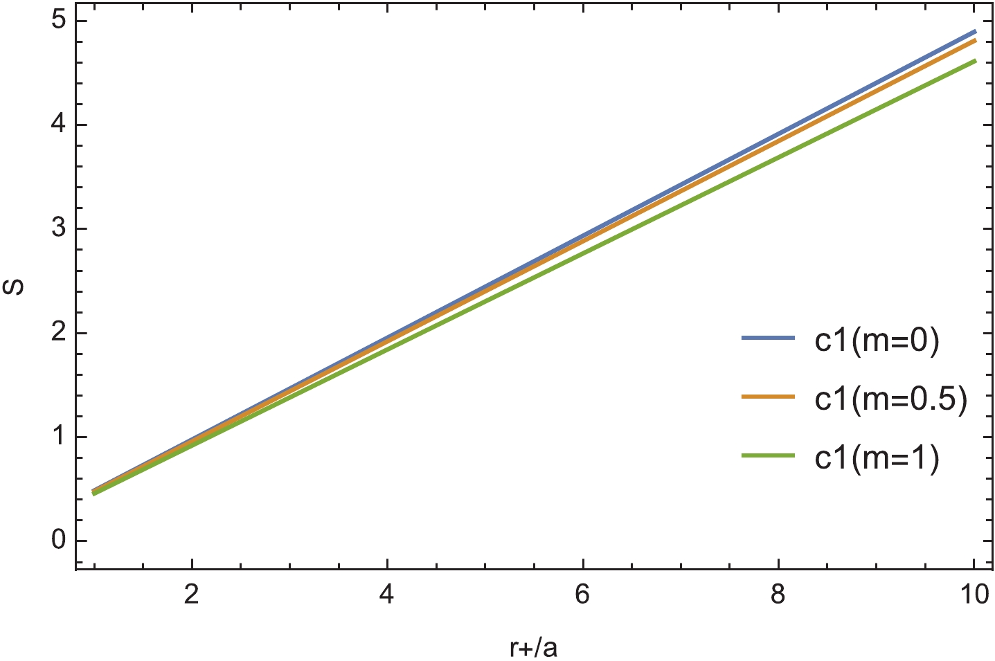
Figure 2. (color online) Linear fitting of the entropy for different m.
-
In this paper, we evaluated the entanglement entropy of a massive BTZ black hole by introducing a massless quantum scalar field using a discretized approach. We found that in all cases,
$S_n$ decreases as n increases, and it is not significant to the total entropy. Meanwhile, when we increase$n_B$ , the entropy increases. The results are very similar to those found in [39]. We also obtained that a larger mass of graviton would reduce the entropy. This means that compared to the theory of massless graviton, the entropy computed by the entanglement entropy in a massive BTZ black hole is suppressed. Furthermore, we fitted the entropy by the quantum correction formula (31) and found the effect of the massive term on the fitting coefficients. The linear coefficient decreases as m increases, which is similar to the effect of the mass of the scalar field obtained in [40]. The subleading coefficient of the log term is suppressed while the constant$c_3$ is enhanced in the massive BTZ black hole. Considering that m also explicitly affects the holographic entanglement entropy in massive gravity, we argued that it is universal that the massive term has a print on the entanglement entropy of a black hole in massive gravity, but the deep physics deserve further study.As it was investigated in [60], it would be very interesting to extend our study by introducing a Fermion field instead of a scalar field into massive gravity and see the effect of the massive term. We shall present the study elsewhere in the near future.
We thank Mahdis Ghodrati for her helpful suggestion on this manuscript.
-
In this appendix, we review the discretized method to calculate the entanglement entropy for scalar fields [25]. Consider a system with coupled harmonic oscillators
$ q^A,\; (A = 1,\cdots,N)$ , the Hamiltonian of which is$\tag{A1} H = \frac{1}{2a}\delta^{AB}p_Ap_B+\frac{1}{2}V_{AB}q^Aq^B. $

Here,
$p^A$ and$p^B$ are canonical momentums conjugate to the$q^A$ and$q^B$ , respectively, which are defined by the relation$p_A = a\,\delta_{AB}\,\dot{q}^B$ with the Kronecker delta$\delta_{AB}$ .$V_{AB}$ is real, symmetric, positive definite matrix and “a” is the fundamental length characterizing the system. By defining a symmetric, positive definite matrix via$V_{AB} = W_{AC}W^C_B$ , one can rewrite the total Hamiltonian as,$\tag{A2} H = \frac{1}{2a}\delta^{AB}\left(p_A+iW_{AC}q^C\right)\left(p_B-iW_{BD}q^D\right)+\frac{1}{2a}\,\mathrm{Tr}\; W. $

The new operators
$(p_{A}+iW_{AC}q^{C})$ and$(p_{B}-iW_{BD}q^{D})$ are the annihilation and creation operators, respectively, which are similar to those of harmonic oscillator problem and they obey similar commutation relation,$[a_A,a_B^{\dagger}] = $ $ 2W_{AB}$ .Then, in the harmonic oscillator system, the ground state
$\psi_{0}$ satisfies$\tag{A3} \left(p_{A}-iW_{AC}q^{C}\right)|\psi_{0}> = 0 $

and the solution is [25]
$\tag{A4} \begin{array}{l} \psi_{0}\left(\{q^C\}\right) =<\{q^C\}|\psi_{0}> = \left[\det\frac{W}{\pi}\right]^{1/4} \mathrm{exp} \left[-\frac{1}{2}W_{AB}\,q^{A}\,q^{B}\right]. \end{array} $

Therefore, the density matrix of the ground state is
$\tag{A5} \begin{split} \rho \left( {\{ {q^A}\} ,\{ {q^{\prime B}}\} } \right) =& < \{ {q^A}\} |0><0|\{ {q^{\prime B}}\} > = {\left[ {{\text{det}}\frac{W}{\pi }} \right]^{1/2}} \hfill \\ &\times {\text{exp}}\left[ { - \frac{1}{2}{W_{AB}}{\mkern 1mu} ({q^A}{\mkern 1mu} {q^B} + {q^{\prime A}}{\mkern 1mu} {q^{\prime B}})} \right]. \hfill \\ \end{split} $

We divide
${q^{A}}$ into two subsystems,${\{q^{a}\}}$ $(a = 1,2,\cdots n_B)$ and$\{q^\alpha\}$ $(\alpha = n_B+1,n_B+2,\cdots N)$ . Then, the reduced density matrix of one subsystem is obtained by tracing the degrees of freedom of the other subsystem as②$\tag{A6} \begin{array}{l} \rho\Big(\{q^{\prime a}\},\{q^{\prime b}\}\Big) = \int\prod\limits_{\alpha}{\rm d}q^{\alpha}\rho\,\Big(\{q^a,q^{\alpha}\},\{q^{\prime b},q^{\alpha}\}\Big). \end{array} $

Thus, the matrix W can be split into four blocks as,
$ \begin{array}{l} (W)_{AB} = \left(\begin{array}{ccc} A_{ab} & B_{a\beta} \\ B^T_{\alpha b} & D_{\alpha \beta}\end{array} \right).\end{array} $

Consequently, the reduced density matrix is rewritten as,
$ \tag{A7} \rho_{\rm red}(\{q^{a}\},\{q^{\prime b}\}) = \left[\mathrm{det}\frac{M}{\pi}\right]^{1/2}e^{-\frac{1}{2}M_{ab}(q^{a}q^{b} +q'^{a}q'^{b})}e^{-\frac{1}{4}N_{ab}(q-q')^a (q-q')^b} $

where
$ \tag{A8} M_{ab} = (A-BD^{-1}B^{T})_{ab} \qquad{\rm and}\qquad N_{ab} = (B^TA^{-1}B)_{ab}. $

The system can be diagonalized by the unitary matrix U , and transformed as
$\tag{A9} \begin{array}{l} q^{a}\rightarrow \tilde{q}^a = (UM^{1/2})^a_bq^{b}. \end{array} $

Thus, the density matrix can be further reduced into [25],
$\tag{A10} \begin{split} {\rho _{\rm red}}(\{ {q^a}\} ,\{ {q^b}\} ) = &\prod\limits_n {\left[ {{\pi ^{ - 1/2}}\exp \left( { - \frac{1}{2}({q_n}{q^n} + q_n^\prime {q^{\prime n}}} \right.} \right.} \hfill \\ & - \left. {\left. {\frac{1}{4}{\lambda _i}{{(q - {q^\prime })}_n}{{(q - {q^\prime })}^n})} \right)} \right], \hfill \\ \end{split} $

where
$ \lambda_i $ are the eigenvalues of the matrix$ \Lambda^a_b = (M^{-1})^{ac}N_{cb} $ . Thus, the entanglement entropy of the system can be calculated using (30) as$ \tag{A11} S_n = -\sum\limits_{i}\ln(\lambda_i^{1/2}/2)+(1+\lambda_i)^{1/2}\ln(1+\lambda_i^{-1}+\lambda_i^{-1/2}). $

Scalar field in massive BTZ black hole and entanglement entropy
- Received Date: 2019-08-18
- Accepted Date: 2019-10-18
- Available Online: 2020-01-01
Abstract: In this paper, we investigate the quantum scalar fields in a massive BTZ black hole background. We study the entropy of the system by evaluating the entanglement entropy using a discretized approach. Specifically, we fit the results with a log -modified formula of the black hole entropy, which is introduced by quantum correction. The coefficients of leading and sub-leading terms affected by the mass of graviton are numerically analyzed.


 DownLoad: