


 Abstract
 HTML
HTML Reference
 Related
 PDF
PDF


-
In recent years, some experimental states or resonances have been announced as observable candidates beyond the conventional quark-antiquark and three-quark configurations. Most of these particles are not confirmed with high statistics and better resolution. Moreover, except for the case for
$ X(3872) $ [1], they were observed only in a single experiment, such as$ X(5568) $ [2, 3] or in one type of experiment, such as B factories. The observation of$ X(3872) $ was a milestone for the era of so-called exotic states. Exotic states are beyond the description of the conventional quark model. The pentaquark represents an example of these exotic states. It consists of four quarks (qqqq) and one antiquark ($ \bar{q} $ ) bound together.This situation turned into a new perspective with the first discovery of the pentaquark candidates,
$ P_c(4450) $ and$ P_c(4380) $ by LHCb in 2015 [4]. Theoretical studies were perfomed for these pentaquark particles prior to their observation [5–8]. The masses of these states were very close to$ \bar{D}^* \Sigma_c^* $ threshold. This justifies the assumption that those two pentaquarks as baryon-meson molecule [9–19]. The other possibilities are the compact pentaquark [20–23], quark model [24–26], chiral quark model [27], quark-cluster model [28] and baryocharmonium model [29].Most recently, the LHCb collaboration updated the results of Ref. [4] reporting the observation of new narrow pentaquark states [30] with masses and widths as follows:
$\begin{aligned} P_c(4312) \; M = & (4311.9 \pm 0.7^{+6.8}_{-0.6}) \;{\rm MeV}, \\ \Gamma =& (9.8 \pm 2.7^{+3.7}_{-4.5}) \;{\rm MeV}, \\ P_c(4440) \; M =& (4440.3 \pm 1.3^{+4.1}_{-4.7}) \;{\rm MeV}, \\ \Gamma =& (20.6 \pm 4.9^{+8.7}_{-10.1}) \;{\rm MeV}, \\ P_c(4457) \; M = & (4457.3 \pm 0.6^{+4.1}_{-1.7}) \;{\rm MeV}, \\ \;\;\;\;\;\;\;\;\;\;\;\;\;\;\Gamma =& (6.4 \pm 2.0^{+5.7}_{-1.9}) \;{\rm MeV}. \end{aligned}$

The masses of
$ P_c(4440) $ and$ P_c(4457) $ are close to$ \Sigma_c \bar{D}^* $ threshold, and the mass of$ P_c(4312) $ is very close to$ \Sigma_c \bar{D} $ threshold. As pointed out in [31], the central mass of the$ P_c(4312) $ state is ~6 MeV below the$\Sigma_c^+\bar{D}^0$ threshold and ~12 MeV below the$ \Sigma_c^{++}D^- $ threshold. For$ P_c(4440) $ , it is ~20 MeV below the$ \Sigma_c^+\bar{D}^{*0} $ and ~24 MeV below the$ \Sigma_c^{++}\bar{D}^{*-} $ thresholds. In the case of$ P_c(4457) $ , it is ~3 MeV below the$\Sigma_c^+\bar{D}^{*0} $ and ~7 MeV below the$ \Sigma_c^{++}\bar{D}^{*-} $ thresholds. The isospin violating process can occur when the width of a resonance is small and mass is below the corresponding thresholds. This can be an example for these pentaquarks.The observation of these pentaquarks received immediate attention [32–39]. In this study, we use the constituent quark model to obtain spectrum and quantum numbers. As mentioned in Ref. [25], the constituent quark model has often been employed for exploratory studies in QCD and paved the way for lattice simulations and QCD sum rules calculations. The main part of the constituent quark model is to obtain a solution of the Schrödinger equation with a specific potential. For mesons and baryons, this can be done effectively, and one can obtain reliable results comparing to the results of experiments. However, pentaquark structures are multiquark systems and due to the complex interactions among quarks, solving the five-body Schrödinger equation is a challenging task. For this purpose, we solved the Schrödinger equation via an artificial neural network (ANN).
Apart from their application in other fields, ANNs can be utilized as an elective strategy to solve differential conditions and quantum mechanical systems [40, 41]. ANNs provide some advantages compared to standard numerical methods [42, 43]
● The solution is continuous over the entire domain of integration,
● With the number of sampling points and dimensions of the problem, the computational complexity does not increase significantly,
● Rounding-off error propagation of standard numerical methods does not influence the neural network solution,
● The method requires a lower number of model parameters and therefore does not require large memory space in computer.
This paper is organized as follows. In Section 2, the model and method used for the calculations are described. In Section 3, obtained results are discussed, and in Section 4, we sum up our work.
-
The Hamiltonian of Ref. [44] reads as follows
$ H = \sum_i \left( m_i+\frac{{p}_{{i}}^{\bf{2}}}{2m_i} \right)-\frac{3}{16}\sum\limits_{i<j} \tilde{\lambda}_i \tilde{\lambda}_j v_{ij}(r_{ij}) $

(1) with the potential
$ \begin{split} v_{ij}(r) =& -\frac{\kappa(1-e^{-\frac{r}{r_c}})}{r}+\lambda r^p + \Lambda + \\& \frac{2\pi}{3m_im_j}\kappa^\prime (1-e^{-\frac{r}{r_c}})\frac{e^{-\frac{r^2}{r_0^2}}}{\pi^{3/2}r_0^3} {\bf{\sigma_i}} {\bf{\sigma_j}}, \end{split}$

(2) where
$ r_0(m_i,m_j) = A \left(\displaystyle\frac{2m_im_j}{m_i+m_j} \right)^{-B} $ , A and B are constant parameters, κ and$ \kappa^\prime $ are parameters,$ r_{ij} $ is the interquark distance$ \vert{ {{r_i}}-{{r_j} \vert}} $ ,$ \sigma_i $ are the Pauli matrices and$ \tilde{\lambda}_i $ are Gell-Mann matrices. There are four potentials referred to the p nd$ r_c $ :$\begin{aligned} {\rm AL1} \to p =& 1, \;\; r_c = 0, \\ {\rm AP1} \to p =& 2/3, \; \; r_c = 0, \\ {\rm AL2} \to p =& 1, \;\; r_c \neq 0, \\ {\rm AP2} \to p =& 2/3,\;\; r_c \neq 0. \end{aligned}$

The related parameters are given in Table 1.
AL1 AP1 AL2 AP2 $ m_u=m_d $ 

0.315 GeV 0.277 GeV 0.320 GeV 0.280 GeV $ m_s $ 

0.577 GeV 0.553 GeV 0.587 GeV 0.569 GeV $ m_c $ 

1.836 GeV 1.819 GeV 1.851 GeV 1.840 GeV $ m_b $ 

5.227 GeV 5.206 GeV 5.231 GeV 5.213 GeV $ \kappa $ 

0.5069 0.4242 0.5871 0.5743 $ \kappa^\prime $ 

1.8609 1.8025 1.8475 1.8993 $ \lambda $ 

0.1653 GeV2 0.3898 GeV5/3 0.1673 GeV2 0.3978 GeV5/3 $ \Lambda $ 

−0.8321 GeV −1.1313 GeV −0.8182 GeV −1.1146 GeV $ B $ 

0.2204 0.3263 0.2132 0.3478 $ A $ 

1.6553 $ {\rm GeV}^{B-1} $ 

1.5296 $ {\rm GeV}^{B-1} $ 

1.6560 $ {\rm GeV}^{B-1} $ 

1.5321 $ {\rm GeV}^{B-1} $ 

$ r_c $ 

0 0 0.1844 $ {\rm GeV}^{-1} $ 

0.3466 $ {\rm GeV}^{-1} $ 

Table 1. Parameters of the potentials.
This potential was developed under the nonrelativistic quark model (NRQM) and used for exploratory studies. It is composed of a 'Coulomb + linear' or 'Coulomb + 2/3-power' term and a strong but smooth hyperfine term. Further details on this potential are provided in Ref. [44]. They built a new interquark potential, which works equally well on the meson and baryon sector. This simple quark model is based on nonrelativistic kinetic energy and a color-additive interaction related to pairwise forces carried by color-octet exchanges [25].
-
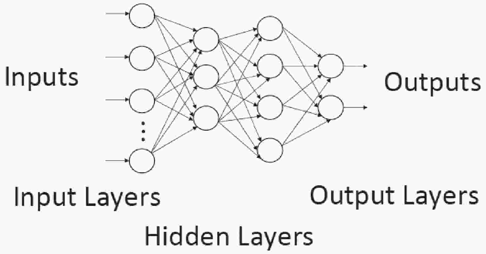
Nowadays, machine learning is one of the most popular research fields of modern science. The fundamental ingredient of machine learning systems is artificial neural networks (ANNs), since the most effective way of learning is done by ANNs. ANN is a computational model motivated by the biological nervous system. ANN is made up of computing units, called neurons. A schematic diagram of an ANN is given in Fig. 1.
Figure 1. A model of multilayer neural networks
In this work, we use a multilayer perceptron (neuron) neural network (MLPN). A MLPN contains more than one layer of artificial neurons. These layers are connected to the next layer, however there is no connection among the neurons in the same layer. They are ideal tools for solving differential equations [45]. A simple model of a neuron can be seen Fig. 2.
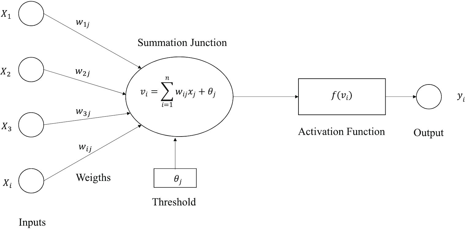
Figure 2. A model of single neuron
Feed-forward neural networks, which are used in this present study, are the most used architectures because of their structural flexibility, good representational capabilities, and a wide range of training algorithms available [45]. All input signals are summed together as z, and the nonlinear activation function determines the output signal
$ \sigma(z) $ . We use a sigmoid function$ \sigma(z) = \frac{1}{1+e^{-z}} $

(3) as an activation function, since all derivatives of
$ \sigma(z) $ can be derived in terms of themselves. The information process can only flow one-way in feed-forward neural networks, namely from input layer(s) to output layer(s). The input-output properties of the neurons can be written as$ o_i = \sigma(n_i), $

(4) $ o_j = \sigma(n_j), $

(5) $ o_k = \sigma(n_k), $

(6) where i, j, and k depict the input, hidden, and output layers, respectively. Input to the perceptrons are given as
$ n_i = ({\rm Input \ signal \ to \ the \ neural \ network}), $

(7) $ n_j = \sum\limits_{i = 1}^{N_i} \omega_{ij}o_i+ \theta_j, $

(8) $ n_k = \sum\limits_{i = 1}^{N_j} \omega_{jk}o_j+ \theta_k, $

(9) where
$ N_i $ and$ N_j $ represent the numbers of the units, which belong to input and hidden layers, respectively,$ \omega_{ij} $ is the synaptic weight parameter connecting the neurons i and j, and$ \theta_j $ is threshold parameter for the neuron j [46]. The overall response of the network can be written as$ o_k = \sum\limits_{j = 1}^{b_n} \omega_{jk}\sigma \left( \sum\limits_{i = 1}^{a_n}\omega_{ij}o_i +\theta_j \right)+ \theta_k. $

(10) One can obtain the derivatives of
$ o_k $ with respect to the network parameters (weights and thresholds) by differentiating Eq. (10) as$ \frac{\partial o_k}{\partial \omega_{ij} } = \omega_{jk} \sigma^{(1)}(n_j)n_i, $

(11) $ \frac{\partial o_k}{\partial \omega_{jk} } = \sigma(n_j)\delta_{kk^\prime}, $

(12) $ \frac{\partial o_k}{\partial \theta_j } = \omega_{jk} \sigma^{(1)}(n_j), $

(13) $ \frac{\partial o_k}{\partial \theta_{k^\prime} } = \delta_{kk^\prime}. $

(14) To obtain the spectra of pentaquark states, we consider the ANN application to a quantum mechanical system. We will follow the formalism that was formulated in [40]. Consider the following differential equation
$ H\Psi(r) = f(r) $

(15) where H is a linear operator,
$ f(r) $ is a function and$ \Psi(r) = 0 $ at the boundaries. To solve this differential equation, it is possible to write a trial function as$ \Psi_t({{r}}) = A({{r}})+B({{r}}, \lambda)N({{r}}, {{p}}), $

(16) which feeds a neural network with vector parameter p and λ to be adjusted later. The parameter p stands for the weights and biases of the neural network.
$ A({{r}}) $ and$ B({{r}}, \lambda) $ should be conveniently specified for$ \Psi_t({{r}}) $ to satisfy the boundary conditions regardless of the p and λ values. To solve Eq. (15), the collocation strategy can be utilized, and it can be changed into a minimization problem as$ \underset{p,\lambda}{\min} \sum\limits_i \left[ H\Psi_t(r_i)-f(r_i) \right]^2. $

(17) Eq. (15) can be written as
$ H\Psi(r) = \epsilon \Psi(r) $

(18) with the boundary condition
$ \Psi(r) = 0 $ . The trial solution can be written of the form$ \Psi_t(r) = B({{r}}, \lambda)N({{r}}, {{p}}), $

(19) where
$ B({{r}}, \lambda) = 0 $ at boundary conditions for a variety of$ \lambda $ values. By discretizing the domain of the problem, Eq. (17) can be transformed into a minimization problem with respect to the parameters p and λ$ E({{p}},\lambda) = \frac{\sum_i \left[ H\Psi_t(r_i, {{p}},\lambda)-\epsilon \Psi_t(r_i, {{p}},\lambda) \right]^2}{\int \vert \Psi_t \vert^2 {\rm d}{{r}}}, $

(20) where E is the error function, and ϵ can be computed by
$ \epsilon = \frac{\displaystyle\int \Psi_t^{\ast} H \Psi_t {\rm d}{{r}}}{\displaystyle\int \vert \Psi_t \vert^2 {\rm d}{{r}}}. $

(21) Considering a multilayer neural network with n input units, one hidden layer with n units and one output, then, for a given input vector
$ {{r}} = \left( r_1, \cdots,r_n \right), $

(22) the output of the network is
$ N = \sum\limits_{i = 1}^m \nu_i \sigma(z_i), $

(23) where
$ z_i = \sum\limits_{j = 1}^n \omega_{ij}r_j+u_i. $

(24) Here,
$ \omega_{ij} $ is the weight from input unit j to hidden unit i,$ \nu_i $ is the weight from hidden unit i to output,$ u_i $ is the bias of hidden unit i and$ \sigma(z) $ is the sigmoid function, Eq. (3). The derivatives of output can be written as$ \frac{\partial^k N}{\partial r^k_j} = \sum\limits_{i = 1}^m \nu_i \omega_{ij}^k \sigma_i^{(k)} , $

(25) where
$ \sigma_i = \sigma(z_i) $ and$ \sigma^{(k)} $ is the k-th order derivative of the sigmoid.To obtain desired results, the ANN has to first perform learning. The learning mechanism is the most important property of the ANN. In this work, we used a feed-forward neural network with a back propagation algorithm, which is also known as delta learning rule. This learning rule is valid for the continuous activation function, such as Eq. (3). The algorithm is as follows [47]:
Step 1 Initialize the weights w from the input layer to the hidden layer and weights v from the hidden layer to the output layer. The learning parameter (that lies between 0 and 1) and error
$ E_{\rm max} $ are chosen. Initially, the error is assumed to be zero.Step 2 Train the network.
Step 3 Compute the error value.
Step 4 Compute the error signal terms of the output layer and the hidden layer.
Step 5 Compute components of error gradient vectors.
Step 6 Check the weights if they are properly modified.
Step 7 If
$ E = E_{\rm max} $ terminate the training session. If not, go to step 2 with$ E \to 0 $ and initiate a new training.We parametrize trial function as
$ \phi_t(r) = r e^{-\beta r^2} N(r, {{u}}, {{w}}, {{v}}), \; \beta >0 $

(26) where N denotes the feed forward artificial neural network with one hidden layer and m sigmoid hidden units with
$ N(r, {{u}}, {{w}}, {{v}}) = \sum\limits_{j = 1}^m \nu_j \sigma(\omega_j r+ u_j). $

(27) The minimization problem becomes as
$ \frac{\sum_i \left[ H\phi_t(r_i)-\epsilon \phi_t(r_i) \right]^2 }{\displaystyle\int \vert \phi_t(r) \vert ^2 {\rm d}r}. $

(28) We solved the Schrödinger equation in the interval
$ 0<r<1 \;{\rm fm} $ using 250 equidistant points with$ m = 10 $ . The wave function Eq. (26) can accommodate the observed meson and baryon spectra. It is apparent that the wave functions for mesons and baryons are different from the pentaquarks. In the case of pentaquark states, the wave function contains not only the spatial part, but also spin, color and isospin parts. To solve the five-body problem, Jacobi coordinates can be used [25]:$ \vec{x} = \vec{r}_2-\vec{r}_1, \; \vec{y} = \vec{r}_4-\vec{r}_3, \; \vec{t} = \vec{r}_5-\frac{\vec{r}_3+\vec{r}_4}{2}, $

(29) $ \vec{z} = \frac{\sum_{i = 1}^2m_i\vec{r}_i}{\sum_{i = 1}^2m_i}-\frac{\sum_{i = 3}^5m_i\vec{r}_i}{\sum_{i = 3}^5m_i}, \; \vec{R} = \frac{\sum_{i = 1}^5m_i\vec{r}_i}{\sum_{i = 1}^5m_i}. $

(30) Quark arrangements with these coordinates are shown in Fig. 3.
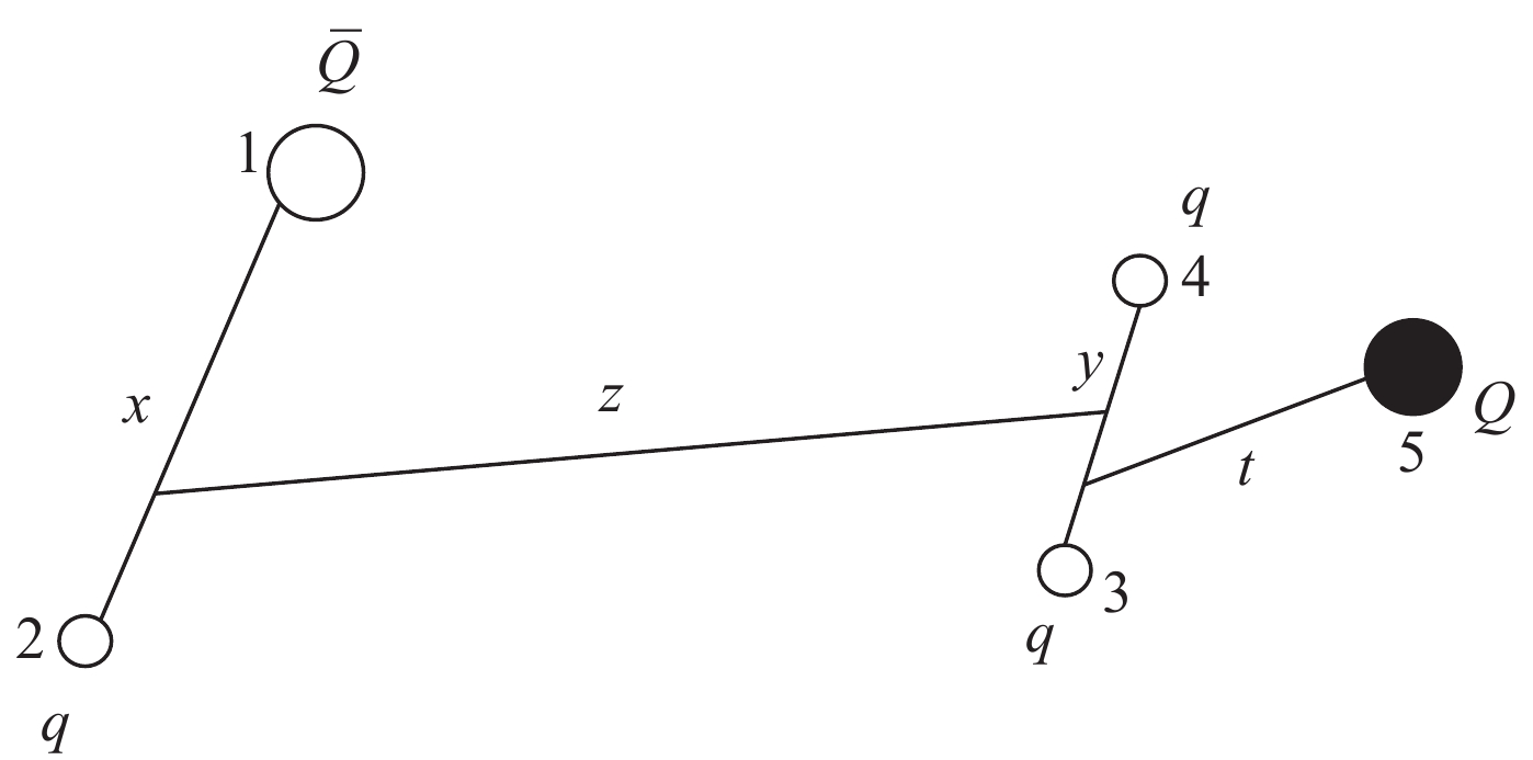
Figure 3. Quark configuration with Jacobi coordinates [25]
In this studfy, we use the wave function of Ref. [25], which reads as
$ \Psi = \sum\limits_{\alpha} \psi_{\alpha} \left(\vec{x},\vec{y},\vec{z},\vec{t} \right) \vert \alpha \rangle , $

(31) $ \psi_{\alpha} \left(\vec{x},\vec{y},\vec{z},\vec{t} \right) = \sum\limits_i \gamma_{\alpha,i} \exp \left(-\tilde{X}^\dagger \cdot A_{\alpha,i} \cdot X/2 \right), $

(32) where
$ \vert \alpha \rangle $ is color spin state,$ A_{\alpha,i} $ are$ 4 \times 4 $ positive definite matrices whose elements are the range parameters, and$ \tilde{X}^\dagger = \left\lbrace \vec{x},\vec{y},\vec{z},\vec{t} \right\rbrace $ . Color states are calculated with the SU(3) Clebsch-Gordan coefficients using the algorithm given in [48]. Taking into account of spin, there are five independent spin arrangements for$ S = 1/2 $ resulting 15 color-spin states$ \vert \alpha \rangle $ , 4 spin states for$ S = 3/2 $ resulting 12 color-spin states, 1 spin state for$ S = 5/2 $ resulting 3 color-spin sates. For the isospin, there are two linearly independent isospin 1/2 vectors and one isospin 3/2 vector. Further discussion on color, spin, and isospin is given in Ref. [26]. The range parameters of$ A_{\alpha,i} $ in the wave function can be used to minimize the energy. For this purpose, we parametrize Eq. (32) as$ \phi_t(x_i) = \sum\limits_i \gamma_{\alpha,i} \exp \left(-\tilde{X}^\dagger \cdot A_{\alpha,i} \cdot X/2 \right) \vert \alpha \rangle N(x_i, {{u}}, {{w}}, {{v}}), $

(33) and the minimization problem becomes
$ \frac{\sum_i \left[ H\phi_t(x_i)-\epsilon \phi_t(x_i) \right]^2 }{\int \vert \phi_t(x_i) \vert ^2 {\rm d}x_i}. $

(34) Before solving the five-body Schrödinger equation, some remarks should be made. At first, the quark configuration in Fig. 3 represents asymptotic thresholds. In this configuration, the pentaquark state is composed of an anti-charmed meson and a charmed baryon. Asymptotic thresholds depict possible nominal reachable values, summing the contribution of all quarks. They are reached when the range parameters of the trial function with the Jacobi coordinate of
$ \vec{z} $ vanish.The second point is that the mass spectrum depends on the choice of the Hamiltoniand and the trial function. In Ref. [26], the authors used a very similar Hamiltonian
$ H = \sum\limits_i \left( m_i+\frac{{{p}}_{{i}}^{\bf{2}}}{2m_i} \right)-\frac{3}{16}\sum\limits_{i<j} \tilde{\lambda}_i \tilde{\lambda}_j V_{ij}(r_{ij}) $

(35) where
$ T_G $ is the kinetic energy of the center-of-mass system and$ V_{ij}(r_{ij}) $ potentials of [44], and with a different wave function. They calculated threshold energies with this Hamiltonian. To test the choice of the Hamiltonian, they also used the AL1 potential of [44] and found that the results of five-body calculations are essentially not modified.Based on these arguments, we solved the Schrödinger equation in the interval
$ 0<x_i<1 \;{\rm fm} $ using 250 equidistant points with$ m = 10 $ . -
At the first step, we calculated the masses of heavy mesons and baryons with all potentials with the wave function given in Eq. (26). The results are given in Table 2.
Meson Exp. AL1 AP1 AL2 AP2 $ \eta_c $ 

2983 2986 2975 2978 2983 $ J/\psi $ 

3096 3095 3100 3091 3096 $ \bar{D} $ 

1869 1862 1876 1860 1868 $ \bar{D}^\ast $ 

2007 2014 2015 2019 2000 Baryon N 938 943 932 936 946 $ \Lambda_c $ 

2286 2285 2290 2283 2279 $ \Sigma_c $ 

2455 2471 2463 2475 2482 $ \Sigma_c^\ast $ 

2520 2525 2541 2534 2533 Table 2. Calculated masses of heavy mesons and baryons. All results are in MeV.
Interestingly, the potential Eq. (2), which has a simple form, i.e., it has no many-body forces and tensor forces, reproduced masses of the observed states quite well. Motivated by these results, we obtained mass values of the newly observed pentaquark states according to their quantum numbers. Table 3 shows the results of
$ J^P = 1/2^- $ case and Table 4 shows$ J^P = 3/2^- $ case, respectively.State Mass AL1 AP1 AL2 AP2 $ P_c(4312) $ 

$ 4311.9 \pm 0.7^{+6.8}_{-0.6} $ 

4314 4317 4320 4312 $ P_c(4440) $ 

$ 4440.3 \pm 1.3^{+4.1}_{-4.7} $ 

4360 4371 4372 4374 $ P_c(4457) $ 

$ 4457.3 \pm 0.6^{+4.1}_{-1.7} $ 

4390 4388 4395 4392 Table 3. Calculated masses of pentaquark states for
$ J^P = 1/2^- $ . All results are in MeV.State Mass AL1 AP1 AL2 AP2 $ P_c(4312) $ 

$ 4311.9 \pm 0.7^{+6.8}_{-0.6} $ 

4371 4382 4377 4369 $ P_c(4440) $ 

$ 4440.3 \pm 1.3^{+4.1}_{-4.7} $ 

4441 4445 4439 4445 $ P_c(4457) $ 

$ 4457.3 \pm 0.6^{+4.1}_{-1.7} $ 

4456 4458 4450 4457 Table 4. Calculated masses of pentaquark states for
$ J^P = 3/2^- $ . All results are in MeV.It can bee seen from Tables 3 and 4 show that the mass of
$ P_c(4312) $ of four potentials with the quantum number assignment$ J^P = \displaystyle 1/2^- $ is more favourable than the quantum number$ J^P = \displaystyle 3/2^- $ . In contrast, the mass of$ P_c(4440) $ and$ P_c(4457) $ with the quantum number assignment$ J^P = \displaystyle 3/2^- $ is more favourable than the the quantum number assignment$ J^P = \displaystyle 1/2^- $ . All the potentials reproduced the experimental data rather well.In addition to the observed states, there are three six states with
$ J^P = 1/2^- $ and$ J^P = 3/2^- $ . We also calculated their mass values, which are shown in Table 5 for$ J^P = 1/2^- $ and in Table 6$ J^P = 3/2^- $ . These states are denoted as$ P_i $ , where$ i = 1,\cdots 6 $ .State AL1 AP1 AL2 AP2 $ P_1 $ 

3978 3964 4005 3994 $ P_2 $ 

4021 4015 4039 4028 $ P_3 $ 

4075 4059 4051 4062 Table 5. Predicted masses of pentaquark states for
$ J^P = 1/2^- $ . All results are in MeV.State AL1 AP1 AL2 AP2 $ P_4 $ 

4099 4102 4114 4089 $ P_5 $ 

4125 4120 4130 4118 $ P_6 $ 

4154 4162 4165 4177 Table 6. Predicted masses of pentaquark states for
$ J^P = 3/2^- $ . All results are in MeV.Two of these states lie below the
$ J/\psi p $ threshold, one of them is above the threshold for$ J^P = 1/2^- $ , and three of them are slightly above the$ J/\psi p $ threshold for$ J^P = 3/2^- $ . This may require a different strategy for observing these states. A further detailed study of the$ J/\psi p $ invariant mass spectrum can elucidate the status of these states.The method of ANN for solving differential and eigenvalue equations includes a trial function [41]. A trial function can be written as a feed-forward neural network, which includes adjustable parameters (weights and biases). The eigenvalue is refined to the existing solutions by training the neural network. As mentioned in Ref. [26], if a wave function results in a multiquark configuration an energy as
$ E = 100 \;{\rm MeV} $ below the lowest threshold, it can represent the exact solution of the system. Moreover, an energy of$ E = 100 \;{\rm MeV} $ above one of the threshold poses a question mark about the wave function and the model for describing the system. The relevant thresholds have been calculated in Ref. [25] as$ 4329 \;{\rm MeV} $ for$ D\Sigma_c $ with$ I(J^P) = \displaystyle\frac{1}{2}(\displaystyle\frac{1}{2})^- $ and$ 4483 \;{\rm MeV} $ for$ D^\ast \Sigma_c $ with$ I(J^P) = \displaystyle\frac{1}{2}(\displaystyle\frac{3}{2})^- $ . Our mass values are below these values, at the order of$ 50 \;{\rm MeV} $ of the relevant thresholds, which means that the trial function of this work represents the five-body structure quite well.The LHCb result could be important to understand the heavy quark spin symmetry (HQSS). In the limit where the masses of heavy quarks are taken to infinity, the spin of the quark decouples from the dynamics, which refers that the strong interactions in the system are independent of the heavy quark spin. This implies that the states that differ only in the spin of the heavy quark, i.e., states in which the rest of the system has the same total angular momentum, should be degenerate. This is also the case for single heavy baryons like
$ \Sigma_c^{\ast} $ $ \Sigma_b^{\ast} $ and referred to as the heavy quark spin (HQS) multiplet structure. Refs. [38, 39] show that the HQS multiplet structure predicts a state near$ \bar{D}^\ast \Sigma_c^\ast $ threshold with$ J^P = 5/2^- $ . The$ \bar{D}^\ast \Sigma_c^\ast $ threshold with$ J^P = 5/2^- $ was calculated in Ref. [25] as$ 4562 \;{\rm MeV} $ . Our mass estimation for this state is shown in Table 7.AL1 AP1 AL2 AP2 Mass 4478 4469 4460 4461 Table 7. Mass prediction of pentaquark state for
$ J^P = 5/2^- $ . All results are in MeV.A
$ 5/2^- $ $ \bar{D}^\ast \Sigma_c^\ast $ state does not couple to the$ J/\psi p $ in S- wave, therefore it is not expected to exhibit a peak in the LHCb [39]. In fact, the phase space rather than partial wave dependence determines whether a state can produce a peak or not. The$ J/\psi p $ threshold is around$ 4040\;{\rm MeV} $ , which is far below the mass of the$ P_c $ state. Given a sufficiently large coupling, this can produce a peak in the$ J/\psi p $ invariant mass spectrum even though the high partial wave is large. Hence, there is still enough room to observe this state. -
Inspired by the recent observation of the hidden-charm pentaquark states, we solved the five-body Schrödinger equation within the nonrelativistic quark model framework. We used a nonrelativistic quark model using the potentials proposed in [44]. These potentials reproduced the experimental ground state masses of some mesons and baryons as a demonstration of the method. We employed the ANN method to obtain the solution of the five-body Schrödinger equation.
We gave a prediction of quantum numbers for these newly observed pentaquarks. The quantum number assignments for
$ P_c(4312) $ ,$ P_c(4440) $ , and$ P_c(4457) $ of this work are in agreement with [33, 34, 36, 38]. Since the spin and parity numbers are not determined in the LHCb report, the other$ J^P $ assignments cannot be excluded. For example, the$ P_c(4440) $ and$ P_c(4457) $ states can be described as$ 5/2^+ $ and$ 5/2^- $ $ \bar{D}^\ast \Sigma_c $ states, respectively [15]. Partial wave analysis in the experimental data is critical to elucidate the internal structures of these exotic states.We also calculated the mass for the
$ 5/2^- $ $ \bar{D}^\ast \Sigma_c^\ast $ state, which is a prediction of heavy quark spin multiplet structure. The average mass value of four estimations is roughly$ 95 \;{\rm MeV} $ below the relevant threshold. Searching this missing HQS partner or partners is an important task for future experiments.Within the framework of Hamiltonian in this study, a molecular picture for the newly observed pentaquark states cannot be concluded or excluded. Both the mass uncertainties and decay properties should be studied. The kinematic vicinity of the observed pentaquark states to the charmed meson-charmed baryon thresholds does not corroborate that they are molecules. In Ref. [49], it is found that masses and decay properties of the
$ P_c(4457)^+ $ ,$ P_c(4440)^+ $ , and$ P_c(4312)^+ $ can be understood if one treats them as$ J^P = 3/2^- $ ,$ J^P = 1/2^- $ and$ J^P = 3/2^- $ , compact pentaquark states, respectively. These properties can also be obtained in the molecule picture, assuming$ J^P = 3/2^- \; (1/2^-) $ ,$ J^P = 1/2^- \; (3/2^-) $ , and$ J^P = (1/2^-) $ S-wave states, respectively.The author thanks to C. Hanhart and the anonymous referee for their valuable comments in the revised version of this paper.
Neural network study of hidden-charm pentaquark resonances
- Received Date: 2019-05-10
- Available Online: 2019-09-01
Abstract: Recently, the LHCb experiment announced the observation of hidden-charm pentaquark states


 DownLoad: