


 Abstract
 HTML
HTML Reference
 Related
 PDF
PDF


-
The observed pulsars [1-3] are generally considered as neutron stars. Most of the observed neutron stars have a mass around 1.4 solar masses (
$ {M}_{\odot} $ ) [4], and PSR J0348+0432 is the heaviest observed neutron star with a precise mass measurement ($ 2.01 \pm 0.04 \, {M}_{\odot} $ ) [5]. From a theoretical perspective, the macroscopic properties of a neutron star, such as the maximum mass ($ M_{{\rm max}} $ ), depend strongly on the equation of state (EOS) of high density matter [6-8].$ M_{\rm max} $ of a neutron star delimits whether it is hydrostatically stable or if it will finally collapse into a black hole through the oscillation process [9]. The recent constraints on$ M_{\rm max} $ , based on the GW170817 observation, are around$ 2.20\; {M}_{\odot} $ . For example, based on the GW170817 observation, three different groups give the constraint on the maximum mass as$ M_{\rm max} < 2.17\; {M}_{\odot} $ [10],$ 2.15\; {M}_{\odot} < M_{\rm max} < 2.25\; {M}_{\odot} $ [11] and$ 2.16\; {M}_{\odot} < M_{\rm max} < $ $2.28\; {M}_{\odot} $ [12]. According to the same gravitational waves (GW) observation, constraint on the radius of a canonical neutron star is given as 11.82 < R1.4/km < 13.72 [13] and constraint on the radius of a neutron star at M =$ 1.6\;{M}_{\odot}$ is R1.6 ≥ 10.7 cm [14].A number of pioneering works have predicted gravitational waves emitted from a binary neutron star (BNS) system [15-17]. The numerical simulations of BNS mergers, with different choices of EOS, illustrate the possibility for indirectly probing the properties of neutron star matter with gravitational waves [18-20]. Postnikov et al. pointed out that the dimensionless tidal deformability
$ \Lambda $ , which can be obtained from the GW signals during the coalescence process of BNS, can characterize different EOS [21]. The first GW detection of BNS coalescence (GW170817) put a constraint on the tidal deformability for canonical neutron stars as$ \Lambda_{1.4} < 800 $ [22] from the first analysis. An improved analysis of GW170817 provided both the upper and lower limits for the tidal deformability as$ {\Lambda _{1.4}} = 190_{ - 120}^{ + 390} $ , which leads to a constraint on EOS at twice the nuclear saturation density as$ p(2{\rho _0}) = 21.85_{ - 10.61}^{ + 16.85} \, \rm{MeV/fm^3} $ [23]. With the observational constraints on$ \Lambda $ , Most et al. generated millions of EOS from their parametrized sets and then exploited more than$ 10^{9} $ equilibrium models for neutron stars to obtain the typical radius$ {R_{1.4}} = 12.39_{ + 1.06}^{ - 0.39} $ $ \rm{km} $ at$ 2\sigma $ level [24].The theoretical determination of
$\Lambda = (2/3){({c^2}/G)^5} $ $ {(R/M)^5}{k_2} $ requires precise inner solutions of the Tolman-Oppenheimer-Volkoff (TOV) equations [25-27]. The relevant tidal Love number$ k_2 $ is determined by the hydrostatic distribution in the stars [25]. The tidal deformability$ \Lambda $ deduced from$ k_2 $ can be used to discriminate EOS. On the other hand, there is no unified model as yet to describe EOS of the compressed matter [28-30]. Even in a specific model, it generally takes complex computations to provide the$ \rho-\varepsilon-p $ relation, where$ \rho $ is the baryon number density,$ \varepsilon $ is the energy density and$ p $ is the pressure. Therefore, numerical EOS tables become a convenient choice in a neutron star study. For the realistic EOS (that is, tabular EOS), the solutions of stellar structures must be obtained by numerical integration.In the integration process, the single-step errors must be restrained to provide accurate results for
$ k_2 $ . In contrast to the integration errors that can be handled simply with shorter step sizes, the interpolation induced errors are mainly affected by the resolution of EOS tables. Nonetheless, when employing a large number of EOS to investigate the neutron star characteristics by Bayesian methods [23, 24, 31, 32], the efficiency of interpolation is of crucial importance. As large size EOS tables are impractical for a statistical study, a suitable resolution for EOS tables becomes particularly important.This paper is organized as follows. In Section 2, a brief introduction of practical techniques for dealing with both the integration and the interpolation is given. Two widely used interpolation methods are introduced to inspect the interpolation induced errors from EOS tables. The minimal size of an EOS table that provides accurate results for
$ M $ and$ \Lambda $ is also discussed. In Section 3, we extend the investigation of different meshing methods for EOS tables to further examine their model dependence. A concise summary is given in the last section. -
In general relativity, the structure of a static, non-rotating and spherically compact star is normally described by the TOV equations. The TOV equations can be written as [26, 27],
$ \displaystyle\frac{{{\rm d}p}}{{{\rm d}r}} = - \displaystyle\frac{{G\left(\varepsilon + \displaystyle\frac{{p}}{{{c^2}}}\right)\left(m(r) + \displaystyle\frac{{4\pi {r^3}p}}{{{c^2}}}\right)}}{{{r^2}\left(1 - \displaystyle\frac{{2Gm(r)}}{{r{c^2}}}\right)}}, $

(2.1) $ \frac{{{\rm d}m(r)}}{{{\rm d}r}} = 4\pi \varepsilon {r^2}, $

(2.2) where
$ m(r) $ refers to the gravitational mass within a radius$ r $ , and$ G $ and$ c $ are the gravitational constant and the speed of light.An important method to investigate the macroscopic properties of neutron stars is to numerically integrate Eqs. (1) and (2) from the center (
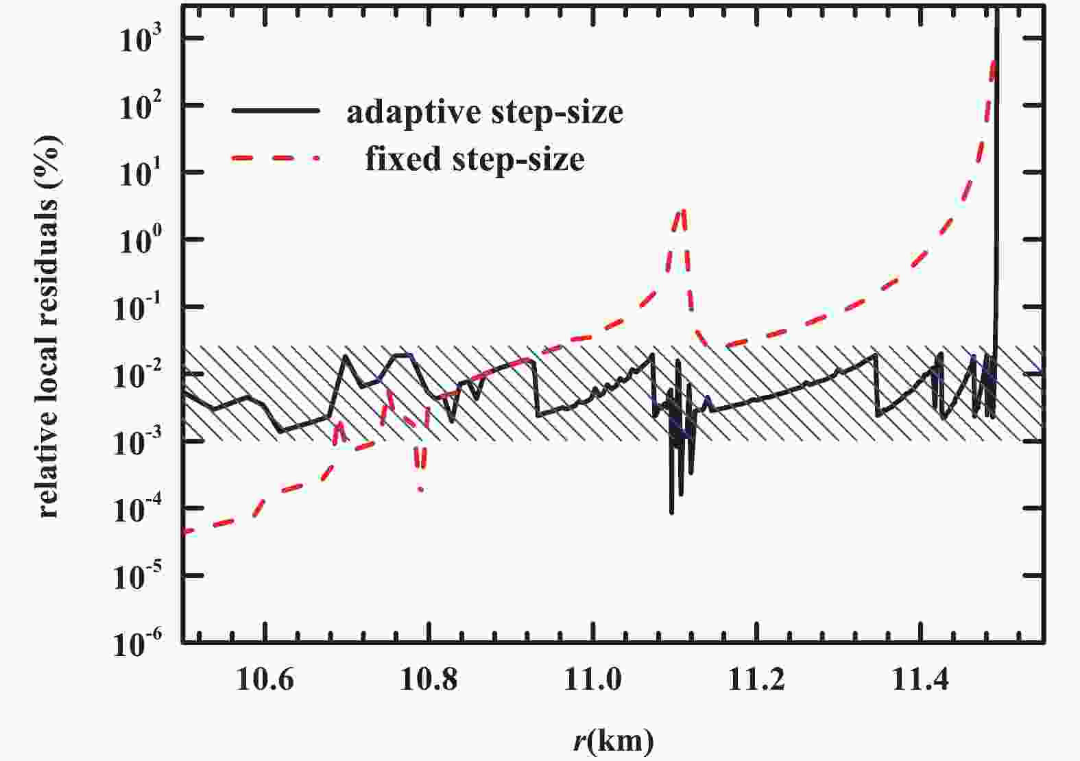
$ m = 0 $ ,$ r = 0 $ ,$ \varepsilon = \varepsilon_c $ ) to the surface ($ p = 0 $ ,$ r = R $ and$ m(R) = M $ ). The widely used forth-order Runge-Kutta (RK-4) method [33, 34] is applied as the high precision integration algorithm in this work. Moreover, we denote the relative deviation of a quantity$ Q $ as$ resQ $ ($ = \left| Q-Q_T \right|/Q_T $ , where$ Q_T $ is the exact value) to discuss its precision.The RK-4 method with adaptive step-size [35-37] can guarantee the global accuracy of the results. In a fixed step-size computation, the local errors at the outer layers can increase rapidly when integrating outwards, which is shown in Fig. 1. The residuals for the final value of the radius are strongly relevant for these errors. The adaptive method effectively controls the local integration errors at the outer crust layer, several meters from the stellar surface. This technique is expected to improve the computational precision significantly at the crust, which is of great concern in investigations of low mass stars. With a proper integration method, the induced radial errors should be <0.1%.
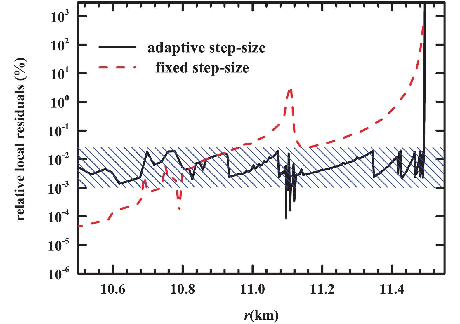
Figure 1. (color online) Relative local residuals for the fixed step-size and adaptive step-size. Relative local residual is defined as the error of pressure increment in each step divided by the exact value of pressure increment. The dashed line represents the fixed step-size (
$h=10\;\rm{(m)}$ ) while the solid line denotes the adaptive step-size. Here, APR EOS is employed and the central density is$4 \rho_0$ .Apparently, the most important input in solving Eqs. (1) and (2) is the
$ \varepsilon - p $ relation. Currently, EOS in tabular form is the most common technique in neutron star investigations. To properly use EOS tables, it is necessary to apply an interpolation method to obtain intermediate values. The errors generated from the interpolation process could be quite different, depending both on the specific method of interpolation and on the resolution of EOS tables.A simple but non-rigorous approximation for EOS tables could be a piecewise polytropic,
$ {\log _{10}}p = {\log _{10}}K + \gamma \left( {{{\log }_{10}}\varepsilon - {{\log }_{10}}{\varepsilon _0}} \right), $

(2.3) where
$ \varepsilon_0 $ ,$ \gamma $ and$ K $ are considered as constant within each segment.In the polytropic approximation, the simplest interpolation is to transform all data points from an EOS table into logarithmic scale and to implement linear interpolation. For example, the value
$ (\varepsilon , p) $ between its nearest neighbors$ (\varepsilon_n , p_n) $ and$ (\varepsilon_{n+1} , p_{n+1}) $ could be given as [38, 39],$ \frac{{{{\log }_{10}}p - {{\log }_{10}}{p_n}}}{{{{\log }_{10}}\varepsilon - {{\log }_{10}}{\varepsilon _n}}} = \frac{{{{\log }_{10}}{p_{n + 1}} - {{\log }_{10}}{p_n}}}{{{{\log }_{10}}{\varepsilon _{n + 1}} - {{\log }_{10}}{\varepsilon _n}}}. $

(2.4) In addition to linear interpolation, an advanced method that simultaneously preserves the monotony and the continuity of the first derivative of EOS is the Piecewise Cubic Hermite Interpolating Polynomial (PCHIP) [40, 41] , which can be written as follows,
$ p\left( \varepsilon \right) = {p_n}{\alpha _n}\left( \varepsilon \right) + {p_{n + 1}}{\alpha _{n + 1}}\left( \varepsilon \right) + {k_n}{\beta _n}\left( \varepsilon \right) + {k_{n + 1}}{\beta _{n + 1}}\left( \varepsilon \right), $

(2.5) where
$ k_{n} $ and$ k_{n+1} $ are the slopes of the interpolated function$ p(\varepsilon) $ at$ \varepsilon_n $ and$ \varepsilon_{n+1} $ , respectively. Specific rules for node slopes$ k_{n} $ are introduced in the Appendix. The four Hermitian functions are given as,$ {\alpha _n}\left( \varepsilon \right) = \left( {1 + 2\frac{{\varepsilon - {\varepsilon _n}}}{{{\varepsilon _{n + 1}} - {\varepsilon _n}}}} \right){\left( {\frac{{\varepsilon - {\varepsilon _{n + 1}}}}{{{\varepsilon _n} - {\varepsilon _{n + 1}}}}} \right)^2} , $

(2.6) $ {\alpha _{n + 1}}\left( \varepsilon \right) = \left( {1 + 2\frac{{\varepsilon - {\varepsilon _{n + 1}}}}{{{\varepsilon _n} - {\varepsilon _{n + 1}}}}} \right){\left( {\frac{{\varepsilon - {\varepsilon _n}}}{{{\varepsilon _n} - {\varepsilon _{n + 1}}}}} \right)^2}, $

(2.7) $ {\beta _n}\left( \varepsilon \right) = \left( {\varepsilon - {\varepsilon _n}} \right){\left( {\frac{{\varepsilon - {\varepsilon _{n + 1}}}}{{{\varepsilon _n} - {\varepsilon _{n + 1}}}}} \right)^2}, $

(2.8) $ {\beta _{n + 1}}\left( \varepsilon \right) = \left( {\varepsilon - {\varepsilon _{n + 1}}} \right){\left( {\frac{{\varepsilon - {\varepsilon _n}}}{{{\varepsilon _n} - {\varepsilon _{n + 1}}}}} \right)^2}. $

(2.9) In order to facilitate the analysis, we divide the tabulated EOS into two parts: the low density segment
$ [0, \rho_0] $ and the supra-nuclear segment$ [\rho_0 , 10\rho_0] $ . In actual calculations, the minimum density is adopted as$ 10^4 $ $ \rm{kg/m^3} $ . For comparison, we define APR-a as the exact EOS, which is spline-fitted from the well-known APR EOS [42] by using a smoothing parameter 0.989 (corresponding to the smallest R-square). To discuss the errors induced by the interpolation process, we uniformly sample from APR-a with logarithmic density in the two segments to produce EOS tables with different resolution. The grid points in each segment are logarithmic-uniform as log10$\, {\rho}_{n+1} $ −log10$ \,{\rho}_n $ = constant. Currently, most of the available EOS tables are provided with grid points of this type (denoted as the$ U $ -grid) in the high density segment [43]. We also use a concise symbol to denote the resolution of an EOS table. For example, APR-20(200) indicates that the table APR EOS contains in total 200 points, with 20 points in the supra-nuclear density segment.We produce EOS tables with sizes 20(200), 20(400), 50(200) and 50(100) from APR-a EOS with the
$ U $ -grid. The relative residuals are estimated with the two interpolation methods mentioned above, and the results are present in Table 1. It is worth pointing out that the integration process is adequately precise if the mass errors are at the level of ~0.001%, which are negligible compared with the interpolation induced errors.exact APR-20(200) APR-50(200) linear PCHIP linear PCHIP $ \rho_c(\rho_0) $ 

$ M(M_{\odot}) $ 

$ resM $ (%)

$ res\Lambda $ (%)

$ resM $ (%)

$ res\Lambda $ (%)

$ resM$ (%)

$ res\Lambda$ (%)

$ resM$ (%)

$ res\Lambda $ (%)

3.3377 1.0900 0.0669 0.3517 0.0887 0.4766 0.0186 0.0624 0.0135 0.0525 4.0071 1.4000 0.4114 2.8483 0.3859 2.4134 0.0458 0.3946 0.0284 0.2269 4.6828 1.6500 0.2489 1.4483 0.1259 0.6086 0.0496 0.4255 0.0253 0.2667 6.7543 2.0500 0.0562 0.2848 0.0104 0.0797 0.0232 0.1820 0.0108 0.1404 Table 1. Relative residuals for the two interpolation methods. The left-most column (
$ \rho_c $ ) is the central density for the corresponding row. The relative residuals$ resM $ and$ res\Lambda $ are defined as the relative deviations of$ M $ and$ \Lambda $ with respect to their exact solutions.As is known, the results for the mass are the most sensitive to EOS in the central region of a star. As shown in Table 1, the smaller
$ resM $ for PCHIP indicates that PCHIP interpolation is advantageous over linear interpolation.exact APR-20(400) APR-50(100) linear PCHIP linear PCHIP $ \rho_c(\rho_0) $ 

$ M(M_{\odot}) $ 

$ resM$ (%)

$ res\Lambda$ (%)

$ resM$ (%)

$ res\Lambda$ (%)

$ resM$ (%)

$ res\Lambda$ (%)

$ resM$ (%)

$ res\Lambda$ (%)

3.3377 1.0900 0.0672 0.3788 0.0894 0.4812 0.0298 0.8041 0.0130 0.3395 4.0071 1.4000 0.4066 2.8416 0.3816 2.4207 0.0465 0.4866 0.0404 0.3764 4.6828 1.6500 0.2313 1.4434 0.1251 0.6026 0.0537 0.5554 0.0408 0.4020 6.7543 2.0500 0.0562 0.2882 0.0103 0.0758 0.0208 0.2742 0.0114 0.0917 The precision of
$ \Lambda $ is affected simultaneously by$ k_2 $ ,$ M $ and$ R $ . In a$ U $ -grid, the precision of$ k_2 $ is generally of the same order as$ M $ , and their relative residuals can be viewed as rough indicators of the precision of the hydrostatic solution. The error of$ R $ is mainly related to the integration step-size, which we will not discuss in detail here, but as a conclusion the relative error of$ R $ is ~0.01% for the four EOS in Table 1. Thus, it is easy to understand that as$ resR \ll resM $ and$ resk_2 \sim resM $ for APR-20(200) and APR-20(400), the relative residual of the Love number is$ \sim 6 \, resM $ .Our calculation shows that for both PCHIP and linear interpolation, the EOS tables with denser data points in the high density segment significantly decrease both the mass and the Love number residuals. The number of data points in APR-20(200) is the same as in APR-50(200), but APR-50(200) produces results which are much more precise due to better resolution in the high density segment. On the other hand, comparing the data for APR-20(400) and APR-20(200) in Table 1, it may be seen that the improvement of the resolution at low densities can not significantly reduce the interpolation induced errors.
These comparisons indicate that the resolution of EOS tables for supra-nuclear densities is much more important than the total number of data points. In addition, we note that a too small size of an EOS table, such as APR-50(100), violates the approximation
$ resk_2 \sim resM $ , and thus reduces the$ \Lambda $ precision, especially for the low mass stars. With additional tests of the resolution in both density segments, the minimal size for the$ U $ -grid APR EOS is finally determined as 50(150), which corresponds to the interpolation induced errors of ~0.02% for$ M $ and ~0.2% for$ \Lambda $ .Actually, a number of EOS used in literature prefer to adopt the table size around 20(200) with the
$ U $ -grid [43], such as SFHo, GShen and LS EOS [44-46]. The interpolation induced errors for the stellar mass$ M $ produced by these EOS tables are expected to be 0.1%~1%. According to the above discussion, it is better that the EOS tables contain more than 50 grid points in the supra-nuclear density segment [$ \rho_0, 10\rho_0 $ ], as they significantly reduce the interpolation induced errors, and thus lead to much more precise solutions for the stellar mass$ M $ and tidal deformability$ \Lambda $ . -
To eliminate accidental factors, we further inspect the interpolation errors for several different grid modes, defined as
$ \frac{{{{\log }_{10}}{\rho _{n + 1}} - {{\log }_{10}}{\rho _n}}}{{{{\log }_{10}}{\rho _n} - {{\log }_{10}}{\rho _{n - 1}}}} = \left\{ {\begin{array}{*{20}{c}} {C_1} ,& {\rm{for }}\; {G{\rm{ - grid}}}\\ {\displaystyle\frac{{1 + {{\rm e}^{ - {C_2} \cdot (n + 1)}}}}{{1 + {{\rm e}^{ - {C_2} \cdot n}}}}} ,& {\rm{for } }\;{ue{\rm{ - grid}}} \end{array}} \right. $

(3.1) where
$ C_1 $ and$ C_2 $ are adjustable coefficients to meet the resolution requirements. Apparently, taking$ C_1 = 1 $ for the$ G $ -grid is equivalent to the$ U $ -grid we mentioned in Section 2.Four different grid modes are defined as follows. (i) For the
$ uu $ -grid, we take$ C_1 = 1 $ in the low density segment and$ C_1 = 0.1 $ in the high density segment. (ii) For the$ ue $ -grid, we adopt$ C_2 = 0.56 $ in the supra-nuclear density segment but use the same grid as the$ uu $ -grid in the low density segment. (iii) For the$ U $ -grid, the EOS table is logarithmic-uniform ($ C_1 = 1 $ ), to be consistent with Section 2. (iv) For the$ G $ -grid,$ C_1 = 0.9785 $ in both density segments. A concise example of the four grids for APR-50(150) is plotted in Fig. 2.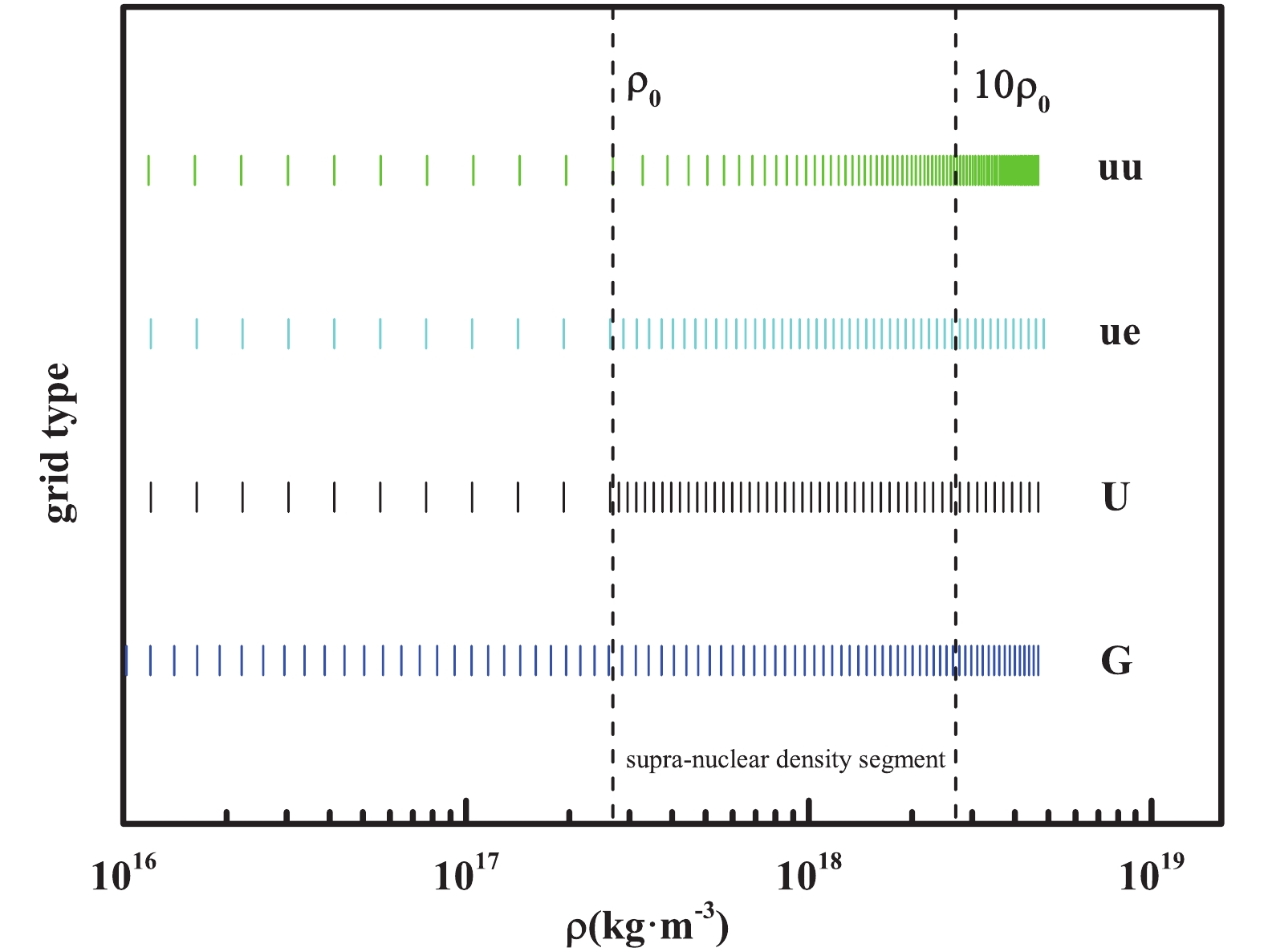
Figure 2. (color online) Baryon density grid points for APR-50(150) and four different grid modes
The
$ uu $ -grid implies a uniform distribution in [$ \rho_0, 10\rho_0 $ ] and logarithmic-uniform in [$ 0, \rho_0 $ ]. It is an extreme distribution where the grid points are concentrated excessively on the high density side. The$ U $ -grid could be considered as the opposite to the$ uu $ -grid. Any distribution that is less contractive than the$ U $ -grid is unjustified according to the discussion in Section 2. From the definitions of the$ G $ -grid and$ ue $ -grid, we see that they are almost transitional schemes between the$ U $ -grid and$ uu $ -grid. The$ ue $ -grid, different from the framework of the$ G $ -grid, is designed to restrain the contraction rate, so that the final interval of the logarithmic grid is expected to be about half of the initial one.From the comparison of the residuals of the four grids shown in Fig. 3, it is clear that the interpolation induced errors are related both to the choice of the EOS mesh and to the central density. For a neutron star, if its central density is near a data point in the EOS tables, it naturally corresponds to a smaller error. For example, the results for the
$ uu $ -grid, which is the most dense on the high density side, are most precise for$ \sim 2 \, {M}_{\odot} $ but least precise on the low mass side. In addition, the interpolation errors of EOS itself are generally small near a data point, and reach a maximum at an intermediate position before the next data point. These regular changes lead to oscillatory contours in Fig. 3.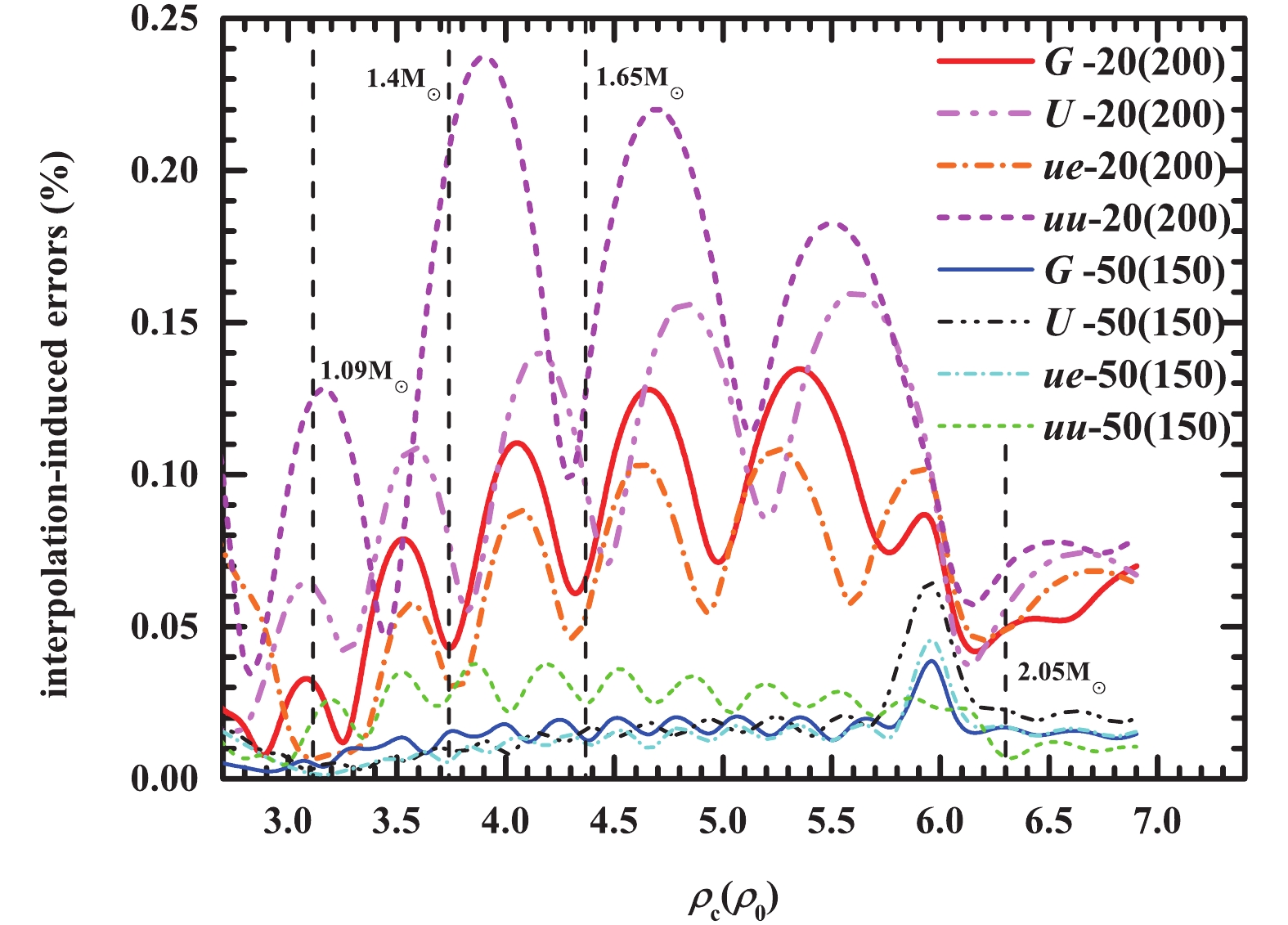
Figure 3. (color online) Residuals of APR-20(200) and APR-50(150) for the four different grids and with PCHIP interpolation. The interpolation induced errors are defined as the relative deviations of
$M$ with respect to the exact solutions.Considering the practicability and overall accuracy, the widely-used
$ U $ -grid remains the optimal choice for EOS tables. Although there is a certain dependence of the accuracy on the meshing method, we may still conclude from Table 1 and Fig. 3 that the EOS tables of size 50(150) could effectively limit the interpolation induced errors of the stellar mass to$ resM\sim $ 0.02% for$1.09 \; {M}_{\odot}< $ $ M<2.05 \; {M}_{\odot} $ .The validity of the above conclusion may be doubted since all EOS tables in our comparison were sampled from a single EOS model. To make the conclusion more reliable, we extended the same interpolation trials to the parametrized asymmetric nucleon matter EOS [47]. We generated several tens of EOS tables in the resolution 50(150), and then estimated the interpolation errors with different methods. We found that they are consistent with the above analyses of APR EOS.
-
We investigated the traditional numerical methods for computing the solutions of the TOV equations including both the integration techniques and the interpolation methods. For convenience of discussion, we separated the global errors into integration errors and interpolation induced errors. As the integration residuals near the stellar surface are divergent and the radial precision can be strongly affected by the choice of step-size, the adaptive step-size method was adopted.
Currently, the bulk of available EOS tables are provided in the general size of
$ \sim20(200) $ [42-46]. As the errors from the integration process can be handled well, the dominant errors when using these EOS tables come from the interpolation process. The relationship between the interpolation induced errors and the resolution of the EOS table with the$ U $ -grid was investigated in detail. It is concluded that increasing the number of data points in the supra-nuclear density segment [$ \rho_0, 10 \rho_0 $ ] can effectively reduce the interpolation induced errors. The EOS table size 50(150) corresponds to the relative residuals for$ M $ and$ \Lambda $ of ~0.02% and ~0.2%, respectively, which is much more accurate than obtained with the size 20(200). In addition, it was also shown that the PCHIP method is more accurate than linear interpolation.The dependence on the meshing methods was also inspected. Among the four proposed meshing methods, the
$ U $ -grid remains the optimal method for generating EOS tables for computing intermediate mass neutron stars. The dependence on the EOS model was also examined using the parametrized asymmetric nucleonic matter EOS [47]. It is concluded that EOS tables with size 50(150) can significantly improve the accuracy compared with the general size 20(200), despite of the differences in the meshing methods, EOS models or interpolation methods. Finally, all source programs (C codes) are publicly available, please refer to Ref. [48].We would like to thank Bao-An Li for helpful discussions.
-
The method used in this work to obtain the nodal slopes
$ k_n $ and$ k_{n+1} $ , used in Eq. (5) for Hermite interpolation, is a weighted average of the nodal slopes$ k_n $ that preserves the shape of the interpolated function at the original data points. The expressions for nodal slopes$ k_n $ at the inner-points and end-points are given in Eqs. (A1)-(A2).In general,
$ k_{n} $ at each node is uniquely determined by the differential properties at the proximal points. Hermite interpolation therefore ensures that the first derivative$ {\rm d}p/{\rm d}\varepsilon $ is continuous everywhere. We denote the right differential step of$ \varepsilon_n $ as$ h_n = \varepsilon_{n+1} - \varepsilon_n $ , and the right differential slope as$ \nu_n = (p_{n+1}-p_n)/h_n $ . When$ sgn(\nu_{n-1}) \ne sgn(\nu_{n}) $ , we choose$ k_n = 0 $ so that the extremum of data points is coincident with the interpolated function, although it is not very likely to have$ sgn(\nu_{n-1}) \ne sgn(\nu_{n}) $ for a rigorous EOS. In the general case,$ k_n $ at the inner-points is given as,$ \tag{A1}\begin{split} \widetilde {{\nu _n}} = \displaystyle\frac{{{h_{n - 1}}{\nu _{n - 1}} + {h_n}{\nu _n}}}{{{h_{n - 1}} + {h_n}}},\\ {k_n} = \displaystyle\frac{{3{\nu _{n - 1}}{\nu _n}}}{{{\nu _{n - 1}} + {\nu _n} + \widetilde {{\nu _n}}}} .\end{split} $

Slope estimation at the two endpoints
$ k_1 $ and$ k_{\rm end} $ is slightly different from the inner-points. We denote the differential step from an endpoint to its nearest neighbor as$ h_{1*} = \varepsilon_{1*}-\varepsilon_{1, {\rm end}} $ , and from the nearest neighbor to sub-neighbor as$ h_{2*} = \varepsilon_{2*}-\varepsilon_{1*} $ , while the corresponding differential slopes are$ \nu _{1*} = (p_{1*}-p_{1,{\rm end}})/h_{1*} $ and$ \nu _{2*} = (p_{2*}-p_{1*})/h_{2*} $ . In the calculations, we first compute$ k_{1, {\rm end}} $ from Eq. (A2). If$ sgn(k_{1, {\rm end}}) \ne sgn(\nu_{1*}) $ we choose$ k_{1, {\rm end}} = 0 $ , else if$ sgn(\nu_{1*}) \ne sgn(\nu_{2*}) $ and$ \left| k_{1, {\rm end}} \right| > \left| 3\nu_{1*} \right| $ we choose$ k_{1, {\rm end}} = 3\nu_{1*} $ , and if the tests above are false$ k_{1, {\rm end}} $ remains invariant.$ \tag{A2}\begin{split}{k_{1, {\rm end}}} = \frac{{\left( {2{h_{1*}} + {h_{2*}}} \right){\nu _{1*}} - {h_{1*}}{\nu _{2*}}}}{{{h_{1*}} + {h_{2*}}}}. \end{split}$

The specific rules for
$ k_{n} $ above are designed to preserve monotony and to avoid overshooting, as the interpolated EOS, in general, is not expected to be oscillatory and barotropic.
Suitable resolution of EOS tables for neutron star investigations
- Received Date: 2018-11-19
- Accepted Date: 2019-02-18
- Available Online: 2019-05-01
Abstract: Inasmuch as the hydrostatic structure of the interior of neutron stars uniquely depends on the equation of state (EOS), the inverse constraints on EOS from astrophysical observations have been an important method for revealing the properties of high density matter. Currently, most EOS for neutron star matter are given in tabular form, but these numerical tables can have quite different resolution. To guarantee both the accuracy and efficiency in computing the Tolman-Oppenheimer-Volkoff equations, a concise standard for generating EOS tables with suitable resolution is investigated. It is shown that EOS tables with 50 points logarithmic-uniformly distributed in the supra-nuclear density segment [


 DownLoad: