


 Abstract
 HTML
HTML Reference
 Related
 PDF
PDF


-
The existence of black holes is theoretically well motivated in general relativity (GR) and other modified theories of gravity. Thus far, black holes have not been directly detected or observed. However, plenty of indirect evidence indicate that such objects exist in nature. As shown by Penrose and Hawking [1], the occurrence of singularities is inevitable in GR. This raises many issues such as the black hole information paradox [2-4] or the more recently discovered paradox of black hole's "firewalls" [5-9]. These paradoxes emerge because of the incompatibility between the quantum theory and GR. It is widely believed that in the quantum theory of gravity, the singularities contained in black holes will be removed. However, even in the early stages of the investigations on singularities [10, 11] in GR, several black hole models, which could avoid the occurrence of a singularity, have been proposed. These black holes are called "regular," because they are singularity-free.
The first proposal of a regular black hole solution was made by Bardeen in Ref. [12], and since then many other models of spherically symmetric regular black holes have been presented in literature [13-21]. In Ref. [22] the authors showed that the Bardeen black hole model can be physically interpreted as the gravitational field produced by a nonlinear magnetic monopole. Later, this interpretation was extended to also include nonlinear electric charges so that regular black holes models can have a nonlinear electromagnetic field as a source. More recently, in Ref. [23] the authors extended the Bardeen solution to an entire class of Bardeen-like black holes that can or cannot be regular.
In this study, the scattering of fermions (spin 1/2) by a Bardeen regular black hole and by a Bardeen-class of black holes (as constructed in [23]) is investigated. We use the partial wave method to obtain analytical expressions for the phase shifts that enter into the definition of partial amplitudes, defining the scattering cross sections and the induced polarization. To the best of our knowledge, this is the first study that reports analytical phase shifts for 1/2-spin wave scattering by regular black holes. The absorption of fermions by Bardeen black holes was numerically investigated in [24], while in Refs. [25-28], the case of massless scalar scattering by regular black holes was also treated numerically. Studies dedicated to fermion scattering by other types of spherically symmetric black holes can be found as examples in Refs. [29-43].
Both Bardeen regular black holes and the Bardeen-class type of black holes possess nonlinear magnetic (monopole) charges [22, 23]. This implies the existence of an electromagnetic potential of the form
$ A=Q_m\cos\theta {\rm d}\phi $ , with$ Q_m $ the total magnetic charge. In this work, we neglect the interaction between this potential and the charge of the fermion and only focus on the scattering due to the "pure" gravitational interaction between the fermion and the black hole. However, even in this approximation, the black hole magnetic monopole charge will still influence the scattering patterns through the presence of$ Q_m $ into the metric function and into the resulting scattering modes of the radial Dirac equation.The remainder of the paper is structured as follows. In Section 2, the Bardeen-class of black holes is presented very briefly. Section 3 begins with a very short review of the Dirac equation in spherically symmetric black hole geometries, and then it discusses the search for scattering modes in the Bardeen spacetime. Finally, the main result of the paper is presented, namely the form of the analytical phase shifts resultant from applying the partial wave method on the scattering modes derived earlier. Section 4 presents a graphical analysis of the induced polarization and the scattering cross sections in which the presence of a backward "glory" and "spiral scattering" (orbiting) oscillations are shown to be present. The main conclusions and some final remarks are presented in Section 5.
-
In Ref. [23], a class of spherically symmetric and asymptotically flat Bardenn-like black holes depending on two-parameters was constructed with the following line element
$ \begin{split} {\rm d}s^2=& h(r) {\rm d}t^2-\displaystyle\frac{{\rm d}r^2}{h(r)}-r^2\left( {\rm d}\theta^2+\sin^2\theta {\rm d}\phi^2 \right), \\ h(r)=& 1-\displaystyle\frac{2M_s}{r}-\displaystyle\frac{2Mr^{\gamma-1}}{\sqrt{(r^2+Q^2)^\gamma}} .\end{split} $

(1) These black holes have a singularity if the parameter
$ M_s $ , hereinafter, referred to as the "Schwarzschild mass," has a nonzero value. Otherwise, if$ M_s=0 $ , regular black holes are obtained and the Bardeen black hole corresponds to the particular choice$ M_s=0 $ and$ \gamma=3 $ . The term M can be interpreted as the mass of the nonlinear magnetic monopole. Moreover, the sum$ M_{\rm ADM}=M_s + M $

(2) constitutes the ADM mass of the black hole obtained from the asymptotic form of the metric function h(r). The parameter Q in Eq. (1) is related to the magnetic monopole charge
$ Q_m $ ;$ Q=2Q_m^2/M $ .As shown in Ref. [23], the Lagrangian density, for which Eq. (1) is a solution of the coupled Einstein-Maxwell filed equations, is given by
$ {\cal{L}}=\frac{4\gamma}{\alpha}\frac{(\alpha F_{\mu\nu}F^{\mu\nu})^{5/4}}{(1+\sqrt{\alpha F_{\mu\nu}F^{\mu\nu}})^{1+\gamma/2}}, $

(3) where
$ \alpha $ has the dimensions of length squared, and$ \gamma $ is a dimensionless constant. In the weak field limit, a vector field, which is slightly stronger when compared with a Maxwell field, is obtained. -
The Dirac equation:
$ i\gamma^a D_a\psi -m\psi = 0 $

(4) The following explicit form can be obtained from the Dirac equation [44]
$ \left( i\gamma^a e^\mu_a\partial_\mu -m \right)\psi + \frac{i}{2}\frac{1}{\sqrt{-g}}\partial_\mu(\sqrt{-g} e^\mu_a)\gamma^a\psi -\frac{1}{4}\{\gamma^a, S^{ b}_{ c} \}\omega^{ c}_{ a b}\psi = 0, $

(5) where
$ g=\det (g_{\mu\nu}) $ and the covariant derivative is defined by$ D_a = \partial_a + \displaystyle\frac{i}{2}S^{ b}_{ c} \omega^{ c}_{ a b} $ .$ S^{a b}=\displaystyle\frac{i}{4}[\gamma^a, \gamma^b] $ the generators of the$ SL(2, \mathbb{C}) $ group,$ \gamma^a $ are the point-independent Dirac matrices obeying$ \{\gamma^a, \gamma^b\}=2\eta^{a b} $ and$ \omega_{ab}^{c} $ is a spin-connection$ \omega^{ c}_{ ab} = e^\mu_a e^\nu_b \left( \hat e^c_\lambda\Gamma^\lambda_{\mu\nu} - \hat e^c_{\nu, \mu} \right) $

(6) $ \Gamma^\lambda_{\mu\nu} $ represents the usual Christoffel symbols. The tetrad fields$ e_a(x) $ and$ \hat e^a(x) $ are point-dependent defining (nonholonomic) local frames and co-frames. The following relations hold:$ \begin{split} & e_a=e_a^\mu\partial_\mu, \;\; \hat e^a=\hat e^a_\mu {\rm d}x^\mu \\ &e_a(x) e_b(x) = \eta_{a b}, \;\; \hat e^a(x) \hat e^b(x) = \eta^{a b} \\ &{\rm d}s^2=\eta_{a b}\hat e^a_\mu {\rm d}x^\mu \hat e^b_\nu {\rm d}x^\nu = g_{\mu\nu}(x) {\rm d}x^\mu {\rm d}x^\nu. \end{split} $

(7) The so-called Cartesian gauge [44-46] for a spherically symmetric line element of the form of Eq. (1) is defined by the following tetrad fields:
$ \begin{split} &\hat e^0 = \sqrt{h} {\rm d}t \\ &\hat e^1 = \displaystyle\frac{1}{\sqrt{h}}\sin\theta\cos\phi {\rm d}r + r \cos\theta\cos\phi {\rm d}\theta - r \sin\theta\sin\phi {\rm d}\phi\\ &\hat e^2 = \displaystyle\frac{1}{\sqrt{h}}\sin\theta\sin\phi {\rm d}r + r \cos\theta\sin\phi {\rm d}\theta + r \sin\theta\cos\phi {\rm d}\phi\\ &\hat e^3 =\displaystyle\frac{1}{\sqrt{h}}\cos\theta {\rm d}r - r \sin\theta {\rm d}\theta, \end{split} $

(8) The Dirac equation (5) can be reduced to only a radial equation. The angular part of the Dirac equation is the same as in the Dirac theory from flat spacetime, and its solutions are the usual four-component angular spinors
$ \Phi^\pm_{m, \kappa}(\theta, \phi) $ [47, 48]. This is because, in the Cartesian gauge (8), the Dirac equation is manifestly covariant under rotations [46]. Using this gauge, it was possible to find complete analytical solutions to the Dirac equation on de Sitter/anti-de Sitter spacetime [49-52] and approximate analytical solutions in black hole geometries [31-33, 53, 54], which were later used to study different aspects of the scattering problem in those spacetimes [31-33, 55-58].The remaining unsolved radial part of the Dirac equation was obtained by assuming the following type of particle-like solutions with a given energy E
$ \begin{split} \psi(x)=& \psi_{E, j, m, \kappa}(t, r, \theta, \phi) \\ =& \displaystyle\frac{{\rm e}^{-{\rm i}Et}}{r h(r)^{1/4}}\left\{ f^+_{E, \kappa}(r)\Phi^+_{m, \kappa}(\theta, \phi) + f^-_{E, \kappa}(r)\Phi^-_{m, \kappa}(\theta, \phi) \right\} \end{split} $

(9) where
$ f^\pm_{E, \kappa}(r) $ are two unknown radial wave functions. As in Refs. [31, 53] the radial Dirac equation can be expressed in a matrix form$ \begin{split} &\left( {\begin{array}{*{20}{c}} {m\sqrt {h(r)} } & { - h(r)\displaystyle\frac{{\rm d}}{{{\rm d}r}} + \displaystyle\frac{\kappa }{r}\sqrt {h(r)} }\\ {h(r)\displaystyle\frac{{\rm d}}{{\rm d}r} + \displaystyle\frac{\kappa }{r}\sqrt {h(r)} } & { - m\sqrt {h(r)} } \end{array}} \right) \\ & \quad \times \left( {\begin{array}{*{20}{c}} {f_{E, \kappa }^ + (r)}\\ {f_{E, \kappa }^ - (r)} \end{array}} \right) = E\left( {\begin{array}{*{20}{c}} {f_{E, \kappa }^ + (r)}\\ {f_{E, \kappa }^ - (r)} \end{array}} \right). \end{split} $

(10) -
Substituting the line element (1) in Eq. (10), we obtain a system of two differential equations that has no analytical solutions owing to the complex form of the line element. However, because we are only interested in finding the scattering modes, we can approximate Eq. (10) in the asymptotic region of the Bardeen black hole specified by the line element in Eq. (1) and find approximative analytical solutions. A partial wave method was used on the obtained solutions to compute the (elastic) scattering cross section and the induced polarization that results after the interaction of a fermion beam with the black hole.
Let us start by introducing the new variable
$ x=\sqrt{\frac{z}{r_+}-1}, \;\; z=\sqrt{r^2+Q^2}, $

(11) where
$ r_+ $ is the radius of the black hole horizon. The function h(r), in terms of x, is$ h=1-\frac{2M_s}{r_+}\frac{1}{\sqrt{(1+x^2)^2-\delta}}-\frac{2M}{r_+}\frac{1}{1+x^2}\left[1-\frac{\delta}{(1+x^2)^2} \right]^{\frac{\gamma-1}{2}} $

(12) where the notation
$ \delta=\left( Q/r_+ \right)^2 $ was introduced. The radial Dirac equation (10) is a system of two differential equations for the radial wave functions$ f^\pm(x) $ that, after multiplying each equation by$ x/[r_+(1+x^2)] $ and expressing all the terms as a function of x given by Eq. (11), is equivalent to Eq. (13)$ \begin{split} & \left[\displaystyle\frac{1}{1+x^2}\sqrt{1-\displaystyle\frac{\delta}{(1+x^2)^2}}\left\{ \frac{ }{ }... \right\}\displaystyle\frac{1}{2}\displaystyle\frac{{\rm d}}{{\rm d}x} + \displaystyle\frac{\kappa}{\sqrt{(1+x^2)^2-\delta}} \right. \times \left.\left\{ \frac{ }{ }... \right\}^{\frac{1}{2}} \right] f^+_{E, \kappa}(x) - \left[\mu \left\{ \frac{ }{ }... \right\}^{\frac{1}{2}} +\epsilon \left(x+\displaystyle\frac{1}{x} \right) \right]f^-_{E, \kappa}(x) = 0 \\ &\quad \left[\displaystyle\frac{1}{1+x^2}\sqrt{1-\displaystyle\frac{\delta}{(1+x^2)^2}}\left\{ \frac{ }{ }... \right\}\displaystyle\frac{1}{2}\displaystyle\frac{{\rm d}}{{\rm d}x}-\displaystyle\frac{\kappa}{\sqrt{(1+x^2)^2-\delta}} \right. \times \left.\left\{ \frac{ }{ }... \right\}^{\frac{1}{2}} \right] f^-_{E, \kappa}(x) - \left[\mu \left\{ \frac{ }{ }... \right\}^{\frac{1}{2}}-\epsilon \left(x+\displaystyle\frac{1}{x} \right) \right]f^+_{E, \kappa}(x) = 0 \\ &\quad{\rm{where}} \;\; \left\{ \frac{ }{ }... \right\}= \displaystyle\frac{(1+x^2)^2}{x^2}-\displaystyle\frac{2M_s}{r_+}\displaystyle\frac{(1+x^2)^2}{x^2\sqrt{(1+x^2)^2-\delta}} -\displaystyle\frac{2M}{r_+}\displaystyle\frac{1+x^2}{x^2} \left[1-\displaystyle\frac{\delta}{(1+x^2)^2}\right]^{\frac{\gamma-1}{2}}, \;\; \mu=r_+ m, \;\; \epsilon=r_+ E . \end{split} $

(13) The system of differential equations obtained in Eq. (13) cannot directly be solved analytically. However, an analytical solution can be obtained if a domain is restricted far away from the black hole event horizon. A simpler system of differential equations that has analytical solutions can be obtained. By Taylor expansion with respect to 1/x and discarding the terms of the order
$ O(1/x^2) $ and higher, the system of equations, which is valid in the asymptotic region of the black hole for the two radial wave function, reduces to$ \begin{split} & \left( \displaystyle\frac{1}{2}\displaystyle\frac{{\rm d}}{{\rm d}x}+\displaystyle\frac{\kappa}{x} \right)f^+_{E, \kappa}(x) - x(\epsilon+\mu)f^-_{E, \kappa}(x) \\ &\quad - \displaystyle\frac{1}{x}\left[\epsilon+ \mu\left(1-\displaystyle\frac{M_{\rm ADM}}{r_+} \right) \right]f^-_{E, \kappa}(x) = 0 \\ & \left(\displaystyle\frac{1}{2}\displaystyle\frac{{\rm d}}{{\rm d}x}-\displaystyle\frac{\kappa}{x} \right)f^-_{E, \kappa}(x) + x(\epsilon-\mu)f^+_{E, \kappa}(x) \\ &\quad + \displaystyle\frac{1}{x}\left[\epsilon-\mu\left(1-\displaystyle\frac{M_{\rm ADM}}{r_+} \right)\right]f^+_{E, \kappa}(x) = 0 . \end{split} $

(14) We observe that if
$ M\rightarrow 0 $ then the ratio$ \displaystyle\frac{M_{\rm ADM}}{r_+}\rightarrow\displaystyle\frac{M_s}{r_s}= \displaystyle\frac{1}{2} $ and$ \mu\left(1-\displaystyle\frac{M_{\rm ADM}}{r_+} \right)\rightarrow\displaystyle\frac{1}{2}\mu $ , recovering the Schwarzschild case discussed in Ref. [53].To find the scattering modes for the case
$ \epsilon>\mu $ , it is useful to introduce new radial wave functions$ \hat f^\pm $ , present in the following combination of the old wave functions$ f^\pm $ $ \begin{split} \hat f^+_{E, \kappa} =& \displaystyle\frac{i}{2}\displaystyle\frac{f^+_{E, \kappa}}{\sqrt{\epsilon+\mu}} +\displaystyle\frac{1}{2}\displaystyle\frac{f^-_{E, \kappa}}{\sqrt{\epsilon-\mu}} \\ \hat f^-_{E, \kappa} =& -\displaystyle\frac{i}{2}\displaystyle\frac{f^+_{E, \kappa}}{\sqrt{\epsilon+\mu}} +\displaystyle\frac{1}{2}\displaystyle\frac{f^-_{E, \kappa}}{\sqrt{\epsilon-\mu}}. \end{split} $

(15) Using the above relation we can obtain the following equations, which are satisfied by the functions
$ \hat f^+_{E, \kappa} $ and$ \hat f^-_{E, \kappa} $ :$ \begin{split} &\left[\nu x\displaystyle\frac{{\rm d}}{{\rm d}x} +2 i\left(\mu^2\left(1-\frac{M_{\rm ADM}}{r_+} \right)-\epsilon^2-\nu^2x^2 \right) \right]\hat f^+_{E, \kappa} \\ &\quad - \left( 2\kappa\nu-i\epsilon\mu\displaystyle\frac{M_{\rm ADM}}{r_+} \right) \hat f^-_{E, \kappa} =0\\ & \left[\nu x\displaystyle\frac{{\rm d}}{{\rm d}x}-2 i\left(\mu^2\left(1-\displaystyle\frac{M_{\rm ADM}}{r_+} \right)-\epsilon^2-\nu^2x^2 \right) \right]\hat f^-_{E, \kappa} \\ &\quad -\left( 2\kappa\nu+i\epsilon\mu\displaystyle\frac{M_{\rm ADM}}{r_+} \right) \hat f^+_{E, \kappa} =0, \end{split} $

(16) where
$ \nu=\sqrt{\epsilon^2-\mu^2} $ . Eq. (16) can now be solved using Maple or Mathematica and the analytical solutions can be written as a combination of Whittaker functions$ \begin{split} \hat f^+_{E, \kappa} =& C_1\displaystyle\frac{1}{x}M_{\rho_+, s}(z)+ C_2\frac{1}{x}W_{\rho_+, s}(z)\\ \hat f^-_{E, \kappa} =& \displaystyle\frac{1}{\kappa^2+\lambda^2}\left[(s-i\alpha)(\kappa+i\lambda)C_1\displaystyle\frac{1}{x}M_{\rho_-, s}(z) \right. \\ & \left.-(\kappa+i\lambda)C_2\displaystyle\frac{1}{x}W_{\rho_-, s}(z)\right], \end{split} $

(17) where
$ z=2i\nu x^2 $ and the following parameters were introduced$ \begin{split} s=&\left[\kappa^2+\mu^2\left(1-\displaystyle\frac{M_{\rm ADM}}{r_+} \right)^2-\epsilon^2 \right]^{\frac{1}{2}}, \;\; \lambda=\frac{\epsilon\mu}{\nu}\cdot\displaystyle\frac{M_{\rm ADM}}{r_+} \\ \rho_{\pm}=&\mp\displaystyle\frac{1}{2} -i\alpha, \;\; \alpha=\displaystyle\frac{1}{\nu}\left[\epsilon^2-\mu^2\left(1-\displaystyle\frac{M_{\rm ADM}}{r_+} \right)\right]. \end{split} $

(18) 3.2.1 Pure Bardeen black hole case
As already mentioned, by choosing
$ M_s=0 $ and$ \gamma=3 $ in Eq. (1) the original Bardeen black hole solution is recovered. This solution is a black hole with two distinct horizons only if$ |Q| < 4/\sqrt{27} $ , it has degenerate horisons if$ Q=4/\sqrt{27} $ and for$ Q>4/\sqrt{27} $ there are no horizons present. Because the function h(r) has now a more simpler form,\begin{equation} h(r)=1-\frac{2Mr^2}{\sqrt{(r^2+Q^2)^3}}, \end{equation}

(19) one can find and write an analytical expression for the location of the black hole outer horizon, denoted from now on by
$ r_+ $ . Moreover, one can easily show that$ r_+=M f(Q/M) $ , where the function f depends only on the ratio Q/M. The existence of horizons implies the constraint$ |Q|/M\leqslant 4/\sqrt{27} $ [14].Following the same steps as in section 3.2, one finds the same scattering modes as given by Eq. (17), but with the new parameters
\begin{equation} \begin{split} s=&\left[\kappa^2+\mu^2\left(1-\displaystyle\frac{M}{r_+} \right)^2-\epsilon^2 \right]^{\frac{1}{2}}, \;\; \lambda=\frac{\epsilon\mu}{\nu}\cdot\frac{M}{r_+} \\ \rho_{\pm}=&\mp\displaystyle\frac{1}{2} -i\alpha, \;\; \alpha=\displaystyle\frac{1}{\nu}\left[\epsilon^2-\mu^2\left(1-\displaystyle\frac{M}{r_+} \right)\right]. \end{split} \end{equation}

(20) We will see in section 4 that this is enough to produce a noticeable difference in the scattering patterns.
By choosing
$ M_s=0 $ and$ \gamma=3 $ in Eq. (1), the original Bardeen black hole solution can be recovered. This solution is a black hole with two distinct horizons only if$ |Q| < 4/\sqrt{27} $ ; it has degenerate horizons if$ Q=4/\sqrt{27} $ , and for$ Q>4/\sqrt{27} $ there are no horizons present. Because the function h(r) can now be expressed in a simpler form: -
In spinor wave scattering theory [48, 59] the differential scattering cross section for an unpolarized incident beam is the sum of the squares of two scalar functions
$ \frac{{\rm d}\sigma}{{\rm d}\Omega}=|f(\theta)|^2 + |g(\theta)|^2, $

(21) which only depend on the scattering angle
$ \theta $ :$ \begin{split} f(\theta)=&\displaystyle\sum_{l=0}^{\infty}\displaystyle\frac{1}{2ip}\left[(l+1)({\rm e}^{2{\rm i}\delta_{-l-1}}-1)+ l({\rm e}^{2{\rm i}\delta_l}-1)\right] \\&P_l^0(\cos \theta), \\ g(\theta)=&\displaystyle\sum_{l=1}^{\infty}\displaystyle\frac{1}{2ip}\left[{\rm e}^{2{\rm i}\delta_{-l-1}}-{\rm e}^{2{\rm i}\delta_l} \right] P_l^1(\cos\theta), \end{split} $

(22) where p is the incident momentum, and
$ P_l^0(\cos\theta), P_l^1(\cos\theta) $ are the Legendre and associated Legendre polynomials, which are special cases of Legendre functions, respectively [60].The phase shifts
$ \delta_l $ can be computed as in Refs. [31, 32] by applying the partial wave method on the scattering modes (17). The asymptotic form of the radial wave functions$ f^\pm $ can be written as [31]$ \left( {\begin{array}{*{20}{c}} {f_{E, \kappa }^ + }\\ {f_{E, \kappa }^ - } \end{array}} \right) \propto \begin{array}{*{20}{c}} {\sqrt {E + m} \sin }\\ {\sqrt {E - m} \cos } \end{array}\left( {pr - \frac{{\pi l}}{2} + {\delta _\kappa } + \vartheta (r)} \right) $

(23) where
$ \vartheta(r)=-p r_++\alpha \ln [2p(r-r_+)] $ represents a radially dependent phase that is independent of any angular quantum numbers; therefore, it does not contribute to the scattering cross sections and may be neglected as in the Dirac-Coulomb case [30, 48].The resultant final form for the point-independent phase shifts
$ \delta_\kappa $ is given by the following expression (see also Appendix A)$ {\rm e}^{2{\rm i}\delta_{\kappa}}=\frac{\kappa-i\lambda}{s-i\alpha}\cdot\frac{\Gamma(1+s-i\alpha)}{\Gamma(1+s+i\alpha)} {\rm e}^{{\rm i}\pi(l-s)}, $

(24) where the sign convention for
$ \kappa $ is the same as in [48], such that$ \kappa=\pm(j+1/2) $ and$ l=|\kappa|-(1-sign \kappa)/2 $ .Series (22) are poorly convergent as a direct consequence of the singularity present at
$ \theta=0 $ ; an infinite number of Legendre polynomials are necessary to describe it. To make the series more convergent, the mth reduced series can be defined$ \begin{split} (1-\cos\theta)^{m_1}f(\theta)= \displaystyle\sum_{l\geqslant 0} a_l^{(m_1)} P_l(\cos\theta), \\ (1-\cos\theta)^{m_2}g(\theta)= \displaystyle\sum_{l\geqslant 1} b_l^{(m_2)} P_l^1(\cos\theta), \end{split} $

(25) as first proposed in [61] and more recently used in [30-32]. The coefficients
$ a_l^{(i)} $ and$ b_l^{(i)} $ are computed using the recurrence relations$ \begin{split} a_l^{(i+1)}=&a_l^{(i)}-\displaystyle\frac{l+1}{2l+3}a_{l+1}^{(i)}-\displaystyle\frac{l}{2l-1}a_{l-1}^{(i)}, \\ b_l^{(i+1)}=&b_l^{(i)}-\displaystyle\frac{l+2}{2l+3}b_{l+1}^{(i)}-\displaystyle\frac{l-1}{2l-1}b_{l-1}^{(i)}, \end{split} $

(26) where
$ a_l^{(0)}=\left[(l+1)({\rm e}^{2{\rm i}\delta_{-l-1}}-1)+ l({\rm e}^{2{\rm i}\delta_{l}}-1)\right]/2ip $ and$ b_l^{(0)}=\left[{\rm e}^{2{\rm i}\delta_{-l-1}}-{\rm e}^{2{\rm i}\delta_{l}} \right]/2ip $ from Eq. (22). We found that using only two iterations$ m_1=2 $ for the function$ f(\theta) $ and one iteration$ m_2=1 $ for$ g(\theta) $ , it is sufficient to make the series converge without distorting the analytical results. -
In this section, we present and discuss the main features of fermion scattering by Bardeen regular black holes and also by a Bardeen-class of black holes. The analysis will focus on scattering by small or micro black holes (with
$ M_{\rm ADM}\sim 10^{15} - 10^{22} $ Kg) because in this case the glory and orbiting scattering phenomena are shown to be significant.The following parameters are used to label the figures:
$ v=p/E $ is the speed of the incident fermions; EM can be considered a dimensionless measure of the gravitational coupling because (restoring the units) it forms the dimensionless quantity:$ \varepsilon=\displaystyle\frac{GEM}{\hbar c^3}=\displaystyle\frac{\pi r_s}{\lambda v} $ , with$ r_s $ the Schwazschild radius and$ \lambda=h/p $ the associated quantum particle wavelength; and the ratios$ q=Q/M_s $ and$ g=M/M_s $ that appear when writing the black hole horizon radius as$ r_+=M_s f\left(\displaystyle\frac{M}{M_s}, \displaystyle\frac{Q}{M_s}\right) $ . Moreover, because in the asymptotic zone$ E=\sqrt{m^2+p^2} $ , one can easily show that$ mM=EM\sqrt{1-v^2} $ such that the condition$ EM\geqslant mM $ is always satisfied. In the following analysis we take$ \gamma=3 $ in all the plots (except those in Fig. 7) because the same conclusions are also obtained for the cases with$ \gamma\neq3 $ .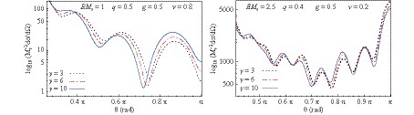
Figure 7. (color online) Comparison of the scattering cross section for a Bardeen-class black hole with different values of the parameter
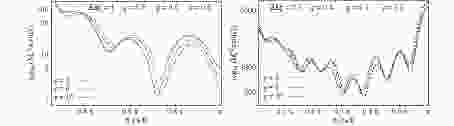
$ \gamma $ . Note that the scattering profile keeps the same shape for different values of$ \gamma $ .In Fig. 1, the differential scattering cross section is presented as a function of the scattering angle for fixed values of the ratios: Q/M (left panels corresponding to pure Bardeen case);
$ q=Q/M_s $ and$ g=M/M_s $ ; a fixed value of the speed (v) of incoming fermions, while the parameter EM (or$ EM_s $ for Bardenn-class) takes different values. From Fig. 1, it can be seen that the scattering pattern takes a simple form for small values of EM. However, as the value of EM increases, more complex scattering patterns occur. This includes the presence of a maximum in the backward direction ($ \theta=\pi $ ), which is also known as "glory" scattering [62, 63] and the presence of oscillations in the scattering intensity that give rise to orbiting or "spiral scattering" [64, 65] (that may occur when the particle's "classical" orbit passes the scattering center multiple times). As the speed of the incoming fermion increases, the peak in the$ \pi $ -direction moves toward the left, and the maximum of the scattering intensity that occurs at$ \theta=\pi $ for nonrelativistic fermions transforms into a minimum if the fermions are massless (v= 1). From the bottom panels of Fig. 1, it can be seen that the magnitude of the spiral scattering oscillations and their angular frequency increase with the black hole mass.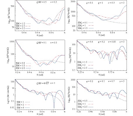
Figure 1. (color online) Plot of the differential scattering cross section as a function of the scattering angle for a regular Bardeen black hole, Eq. (19) (left panels) and for a Bardeen-class black bole, Eq. (1) (right panels). Phenomena of glory (scattering in the backward direction) and spiral scattering (oscillations in the scattering intensity) are present for both types of black holes. The value
$ q/M_{em}=4/\sqrt{27} $ corresponds to a degenerate regular Bardeen black hole (it has only one horizon). The parameter q gives the ratio$ q=Q/M_s $ and$ g=M/M_s $ is the ratio between the magnetic monopole mass and the "Schwarzschild mass".The scattering cross section
$ {\rm d}\sigma/{\rm d}\Omega $ for the Bardeen-class black holes (1) is plotted in Fig. 2. The left panels show the scattering patterns for Bardeen-class black holes that have the "Schwarzschild mass" greater than the mass of the magnetic monopoles, while the right side panels show those with a lower mass. By comparing our analysis results with the Schwarzschild black hole, the scattering intensity in the backward direction ($ \theta=\pi $ ) is higher for the scattering by a Bardeen-class black hole. From Fig. 2, one can also observe that in all the plots, the value of g increases as the number of oscillations of the scattering intensity increases. Furthermore, if we assume$ M_s $ is fixed, then the ADM-mass of the black hole increases (which is equivalent to increasing the mass M, Eq. (2), if$ M_s $ remains constant), and as a consequence the angular frequency of the oscillations present in the scattering intensity also increase. This feature was also true for fermion scattering by Schwarzschild and Reissner-Nordström black holes [30-33]. Thus, the increase in the frequency of the oscillations of the spiral scattering with the black hole mass for any type of (spherically symmetric) black holes is of interest.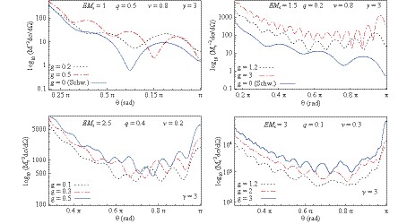
Figure 2. (color online) Variation of the scattering cross section with the parameter
$ g=M/M_s $ for given values of$ EM_s $ and v. In the top panels, the Schwarzschild scattering (for which g= 0) is compared. The value of g increases as the spiral scattering becomes more pronounced.Comparing the scattering intensity, in Fig. 3, of a Bardeen regular black hole (blue and red curves) with that of a Schwarzschild black hole (the black dotted curve), we observe that the glory peak is higher for the scattering by a Schwarzschild black hole. As the ratio Q/M increases, the maximum in the backward direction becomes lower, and the frequency of the oscillations in the spiral scattering slightly decrease simultaneously. The curve with
$ Q/M=4/\sqrt{27} $ corresponds to the Bardeen degenerate case when only one horizon is present. The type of black hole can be determined by analyzing the patterns in the scattering intensity when the scattering of a beam of fermions by a black hole can be observed and measured. If it is a Bardeen black hole, with a known mass, then the value of Q can also be found.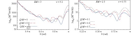
Figure 3. (color online) Scattering cross section for a regular Bardeen black hole for different values of Q/M, while the parameters EM and v are kept fixed.
In Fig. 4, we plotted the differential scattering cross section
$ \displaystyle\frac{{\rm d}\sigma}{{\rm d}\Omega} $ as a function of the scattering angle$ \theta $ for a Schwarzschild black hole (blue solid lines), regular Bardeen black hole (black dotted lines) and Bardeen-class black hole (red dash-dotted lines).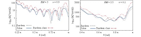
Figure 4. (color online) Comparison between the fermion scattering by a Schwarzschild black hole, regular Bardeen black hole, and Bardeen-class black hole. For the left panel Q/M= 0.2, q= 0.2, and g= 0.5 were used, while for the right panel Q/M= 0.4, q= 0.1, and g= 0.2.
An incident unpolarized beam of massive fermions becomes partially polarized after it gets scattered by the black hole. The induced polarization degree can be computed using the following formula [30, 59]
$ {\vec {\cal {P}}} = - i\frac{{f{g^*} - {f^*}g}}{{|f{|^2} + |g{|^2}}}\vec n $

(27) where
$ \vec n $ is a unit vector in a direction orthogonal to the plane of scattering.In Fig. 5, the dependence of the polarization on the scattering angle is plotted for given values of the parameters EM, v, g, and Q/M. It has a pronounced oscillatory behavior. From the top panels in Fig. 5, one can observe that if the parameter EM increases, then the frequency of the oscillations present in the polarization increases as well. Now, if we assume that the energy of the fermion is fixed, then, the oscillations present in the polarization are more pronounced for black holes with higher masses. Compared with the Schwarzschild polarization (see bottom panels in Fig. 5) the Bardeen and Bardeen-class black hole polarizations exhibit a slightly less oscillatory behavior. The oscillations present in the polarization can be observed as a consequence of the oscillations present in the glory and spiral scattering.
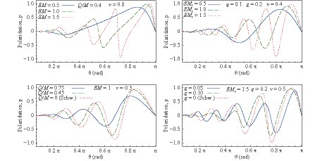
Figure 5. (color online) Partial polarization
$ \cal{P} $ as a function of the scattering angle$ \theta $ . Top left panel: typical Bardeen black hole (19) with Q/M= 0.4 for incoming fermions with speed v= 0.8 in units of c; Top right panel: Bardeen-class black hole (1) with$ g=M/M_s=0.2 $ for incoming fermions with speed v=0.4 in units of c; Bottom left panel: comparing Schwarzschild and pure Bardeen black hole polarizations for fixed EM= 1 and v= 0.3; Bottom right panel: comparing Schwarzschild and Bardeen-class black hole polarizations for fixed$ EM_s=1.5 $ ,$ q=Q/M_s=0.2 $ and v= 0.5.The alignment of the scattered fermions with the forward on-axis direction can be visualized using the polar plots representations of the polarization degree as shown in Fig. 6. One can observe the Mott polarization in the direction orthogonal to the scattering plane, a phenomena that has been reported before in literature for Schwarzschild [30, 31] and Reissner-Nordström [32] black holes.

Figure 6. (color online) Polar plots of pure Bardeen (left panel) and Bardeen-class (right panel) polarization
$ {\cal{P}}(\theta) $ for$ 0 \leqslant\theta\leqslant 2\pi $ showing the alignment of the scattered fermion's spin with a given direction. The Mott polarization (polarization in the direction orthogonal to the scattering plane) can also be observed.In Fig. 7, the differential scattering cross section is plotted for a Bardeen-class black hole with different values of the parameter
$ \gamma $ . Note that the scattering pattern maintains the same profile shape, and the difference between the values of$ {\rm d}\sigma/{\rm d}\Omega $ (computed using different values of$ \gamma $ ) is very small. Moreover, from our analysis results, it can be seen that, for most cases, this difference is even smaller than for the examples presented in Fig. 7. This can be attributed to the difference between the black hole horizon radii$ r_+ $ obtained for different values of$ \gamma $ (while all the other parameters are kept constant) is very small. -
We studied the scattering of fermions by a class of Bardeen black holes that also include the original Bardeen regular black hole solution. A partial wave method was used on a set of scattering modes that were obtained by solving the Dirac equation in the asymptotic region of these black hole geometries. TO the best of our knowledge, for the first time, time analytical phase shifts for fermion scattering by Bardeen regular black holes were obtained. The phenomena of glory (scattering in the backward direction) and spiral scattering (oscillations in the scattering intensity) were also discussed. We also saw that an incident unpolarized beam could become partially polarized after interaction with a black hole.
In Figs. 1-6, other than the parameters EM (that can be associated with a measure of the gravitational coupling) and v (speed of the fermion) we also used the ratios Q/M,
$ q=Q/M_s $ , and$ g=M/M_s $ to label the figures. The departure of the scattering pattern from the Schwarzschild case was significant as Q/M and g increased. For the original Bardeen regular black hole,$ Q/M=4/\sqrt{27} $ was the maximum allowed value, and it corresponds to the degenerate case when the two horizons coincide. If the magnetic charge$ Q\rightarrow 0 $ , then$ M\rightarrow 0 $ and$ g\rightarrow 0 $ , and the scattering by a Schwarzschild black hole can be recovered [31].The glory and spiral scattering become significant for values of the parameter EM~1 or greater (in geometrical units with
$ G=\hbar=c=1 $ ) because the associated wavelength for these values of the incident fermions is of the same order of magnitude as the black hole horizon radius; thus, diffraction patterns occur. Another feature, which was also shown to be present for fermion scattering by Schwarzschild [30, 31] and Reissner-Nordström black holes [32], is that as the total mass of the black hole increases, the oscillations present in the scattering intensity become more frequent, that is, spiral scattering is significantly enhanced with an increase in black hole mass. -
The aim of this Appendix is to briefly present how the phase shifts (24) are obtained.
The asymptotic representation of the Whittaker function
$M $ for large values of |z| is given by the following equation [60]$ \tag{A1} \begin{split} M_{\kappa, \mu}(z)\sim& \frac{\Gamma(1+2\mu)}{\Gamma\left(\frac{1}{2} +\mu-\kappa\right)}{\rm e}^{\frac{1}{2}z}z^{-\kappa}\left(1+O(z^{-1})\right) \\ & +{\rm e}^{{\rm i}(\frac{1}{2}+\mu-\kappa)\pi}\frac{\Gamma(1+2\mu)}{\Gamma\left(\frac{1}{2}+\mu+\kappa\right)} {\rm e}^{-\frac{1}{2}z}z^{\kappa}\left(1+O(z^{-1})\right) \end{split} $

valid for
$ -\frac{1}{2}\pi < {\rm ph }z < \frac{3}{2}\pi $ .To obtain the phase shifts (24), the condition
$ C_2=0 $ must be imposed on Eq. (17) in order to obtain the correct Newtonian phase shifts for large values of angular momenta. As an observation, this condition also selects the spinors that are regular in x= 0 owing to the regularity of the function$ M_{\rho_{\pm}, s}(2i\nu x^2)=(2i\nu x^2)^{s+\frac{1}{2}}[1+O(x^2)] $ . More arguments for letting$ C_2=0 $ can be found in Appendix C of our previous paper [31].Using Eq. (28) on the
$ \hat f^\pm(x) $ functions and by observing that for$ \hat f^+ $ the dominant term is the first one in (28), while for$ \hat f^- $ the second term is dominant, then one obtains the following asymptotic expressions$ \tag{A2} \begin{split} \hat f^+(x)\to& C_1 {\rm e}^{-\frac{1}{2}\pi \alpha}\frac{\Gamma(2s+1)}{\Gamma(1+s+i\alpha)} {\rm e}^{{\rm i}[\nu x^2+\alpha\ln(2\nu x^2)]}\\ \hat f^-(x)\to& \frac{(s-i\alpha)(\kappa+i\lambda)}{\kappa^2+\lambda^2}C_1{\rm e}^{-\frac{1}{2}\pi \alpha}\frac{\Gamma(2s+1)}{\Gamma(1+s-i\alpha)}\\ &\times {\rm e}^{-{\rm i}[\nu x^2+\pi s+\alpha\ln(2\nu x^2)]}. \end{split} $

The last step is to compute the argument of the trigonometric functions (23) as
$ \frac{1}{2}{\rm arg}\left(\frac{\hat f^+}{\hat f^-}\right) $ from which the expression for$ {\rm e}^{2{\rm i}\delta_{\kappa}} $ will result.
Fermion scattering by a class of Bardeen black holes
- Received Date: 2018-10-03
- Accepted Date: 2018-12-29
- Available Online: 2019-03-01
Abstract: In this study, the scattering of fermions by a class of Bardeen black holes is investigated. After obtaining the scattering modes by solving the Dirac equation in this geometry, we use the partial wave method to derive an analytical expression for the phase shifts that enter into the definitions of partial amplitudes that define the scattering cross sections and induced polarization. It is shown that, similar to Schwarzschild and Reissner-Nordström black holes, the phenomena of glory and spiral scattering are present.


 DownLoad: