


 Abstract
 HTML
HTML Reference
 Related
 PDF
PDF


-
The cosmological principle assumes that our Universe is homogeneous and isotropic on large scale, which is one of the foundations of modern cosmology [1]. During the past few decades, the cosmological principle has been tested many times and found to be well consistent with most cosmological observations, for instance, the halo power spectrum [2], the statistics of galaxies [3], the cosmic microwave background (CMB) radiation from the Wilkinson Microwave Anisotropy Probe (WMAP) [4, 5] and the Planck satellites [6–8]. However, there are still some phenomena which are inconsistent with the cosmological principle, such as the alignment of the quasar polarization vectors on large scale [9], the spatial variation of the fine structure constant [10, 11] and the MOND acceleration scale [12–14], the anisotropic accelerating expansion of the Universe [15–20], the alignment of the CMB quadrupole and octupole [21–23], the hemispherical power asymmetry in CMB [24–27], and parity asymmetry in CMB [26–31]. In particular, hemispherical power asymmetry, initially observed by WMAP [4, 5], is one of the outstanding anomalies that indicates violation of statistical isotropy on large angular scales of the CMB sky. This anisotropic signal persisted in Planck [26, 27]. The hemispherical power asymmetry has been modeled as a dipole modulation of the otherwise statistically isotropic CMB sky,
$ \Delta \tilde{T}(\hat{ n}) = \Delta T(\hat{ n})(1+A\hat{ \lambda} \cdot \hat{ n}) $ , where$ \Delta \tilde{T}(\hat{ n}) $ is the modulated/observed CMB field in the direction$ \hat{ n} $ , and$ \Delta T(\hat{ n}) $ is the isotropic CMB field in the same direction. A and$ \hat{ \lambda} $ are the amplitude and direction of modulation. The recently released data of the Planck collaboration show deviations from isotropy with a level of significance of$ \sim3\sigma $ [26]. These phenomena may imply the existence of cosmic anisotropy.As standard candles [32, 33], the supernovae of type Ia (SNe Ia) have been used in a number of works to examine the cosmological principle [16, 18–20, 34–58]. In these studies, the most commonly used datasets are the Union2 sample [59], Union2.1 sample [60] and "Joint Light-curve Analysis" (JLA) compilation [61]. Certain preferred directions were found in the Union2 sample by the hemisphere comparison method [16, 18–20, 34, 38, 41, 44, 47]. The dark energy dipole was found at the 2
$ \sigma $ level in the Union2 sample [39]. Zhao et al. [42] found the dipole of the deceleration parameter at more than the 2$ \sigma $ level by dividing the Union2 sample into 12 subsets. A dataset composed of SNe Ia with$ z<0.5 $ in Union2 was shown to deviate from the ΛCDM model at the$ 2\sigma\sim3\sigma $ level [37]. Contrary to the Union2 sample, the JLA sample does not give any convincing signal of deviation from the isotropic universe. Wang et al. [55] used the JLA sample to constrain the anisotropic universe model with the Bianchi-I metric and found that the model was consistent with the isotropic universe. Constraining the anisotropic amplitude and direction in three different cosmological models of dark energy with the JLA sample gave a zero result [50]. Chang et al. [57] performed a tomographic analysis of the JLA sample by taking account of the redshift dependence of the SNe Ia color-luminosity parameter$ \beta $ in the dipole-modulated ΛCDM model, but they did not find any significant deviation from the isotropic universe.Recently, the Pantheon supernovae sample was released [62] , which consists of 1048 spectroscopically confirmed SNe Ia covering the redshift range
$ 0.01<z<2.26 $ . Compared to the Union2 and JLA samples, the number of SNe Ia in the Pantheon sample is enlarged. The distribution of SNe Ia in Pantheon are inhomogeneous, and half of them are located in the south-east of the galactic coordinate system. The systematic uncertainties were reduced by cross-calibration between subsamples in Pantheon. Therefore, the Pantheon sample could bring a much stronger constraint for the anisotropy of the Universe. Previously, the Pantheon sample has been used to test the cosmological principle. Sun et al. [63] used the redshift tomography method to investigate the cosmic anisotropy in the Pantheon sample, and found that the isotropic cosmological model is an excellent approximation. No evidence of cosmic anisotropy was found in the Pantheon sample by using the hemisphere comparison method, the dipole fitting method and HEALPix [64]. Zhao et al. [65] investigated the cosmic anisotropy in five combinations of Pantheon, and found that the Low-$ z $ and SNLS subsamples have a decisive impact on the hemisphere anisotropy, while the SDSS subsample has a decisive impact on the dipole anisotropy. All these tests are based on the ΛCDM cosmological model. We study whether cosmic anisotropy appears in other cosmological models. In this paper, the Pantheon sample is used to constrain the possible dipole anisotropy in four cosmological models, which include the Finslerian cosmological model, the dipole-modulated ΛCDM, wCDM and Chevallier–Polarski–Linder (CPL) models. We use the MCMC method to explore the whole parameter space and find out the best fit parameters.The paper is arranged as follows. In Section 2, we briefly introduce the Pantheon sample and the four anisotropic cosmological models. In Section 3, we show the constraints for the four anisotropic cosmological models. Finally, the conclusions are given in Section 4.
-
In the spatially flat spacetime, the distance modulus is defined as
$ \mu_{\rm t h} = 5 \log _{10} \frac{d_{L}}{\rm{Mpc}}+25, $

(1) where the luminosity distance is given as
$ d_{L} = \left(c / H_{0}\right) D_{L} $ ,$ H_0 $ is the Hubble constant, c is the speed of light and$ D_{L} $ takes the form,$ D_{L} = \left(1+z_{\rm cmb}\right) \int_{0}^{z_{\rm c m b}} \frac{{\rm d} z}{E(z)}, $

(2) where
$ z_{\rm cmb} $ denotes the CMB frame redshift. The expression for$ E(z) $ varies in different cosmological models. In the ΛCDM model,$ E(z) $ is given as$ E^2(z) = \Omega_{m}(1+z)^3+(1-\Omega_{m}), $

(3) where
$ \Omega_m $ is the matter density in the present epoch. In the wCDM model,$ E(z) $ is given as$ E^2(z) = \Omega_{m}(1+z)^{3}+\left(1-\Omega_{m}\right)(1+z)^{3(1+w_0)}, $

(4) where
$ w_0 = p/\rho $ is the equation of state of dark energy. If$ w_0 = -1 $ , the wCDM model reduces to the ΛCDM model. In the CPL parametrization [66, 67], the equation of state of dark energy is redshift-dependent,$ E(z) $ takes the form$ \begin{array}{l} {E^2}(z) = {\Omega _m}{(1 + z)^3} + \left( {1 - {\Omega _m}} \right){(1 + z)^{3\left( {1 + {w_0} + {w_1}} \right)}}\\ \;\;\;\;\;\;\;\;\;\;\;\;\;\;\; \times \exp \left( { - 3{w_1}\displaystyle\frac{z}{{1 + z}}} \right). \end{array}$

(5) The CPL model reduces to the wCDM model when
$ w_1 = 0 $ .Contrary to the ΛCDM, wCDM and CPL models, there exists a preferred direction in the Finsler spacetime which breaks the isotropy of the Universe [18, 45, 48, 68]. The cosmic anisotropy could originate from the anisotropic background spacetime. Finsler spacetime admits less symmetry than the Riemann spacetime, and is a possible candidate for investigating the cosmologically preferred direction and the dipole structure [69–72]. We previously proposed a Finsler spacetime scenario of the anisotropic universe, which gives a unified description of the dipoles of the fine-structure constant and of the SNe Hubble diagram [48]. It is interesting to test the Finsler spacetime scenario in the newly released SNe data. In a specific Finsler spacetime, i.e. the Randers spacetime, the scale factor has the form
$ a = (1+A_{\rm D}\cos\theta)/(1+z) $ , where$ A_{\rm D} $ is a parameter of the Randers metric which can be regarded as the dipole amplitude. When$ A_{\rm D} = 0 $ , the Randers metric reduces to the FLRW metric, and the Finslerian cosmological model reduces to the ΛCDM model. More details of the Finsler spacetime scenario can be found in [48]. Correspondingly,$ E(z) $ then has the form$ E^2(z) = \Omega_{m}(1+z)^3(1-3A_{\rm D} \cos \theta)+(1-\Omega_{m}), $

(6) where
$ \theta $ is the angle between the preferred direction in the Finsler spacetime and the position of SNe Ia. In the galactic coordinate system, the parametrization of the Finslerian preferred direction is the same as the dipole direction$ \hat{{ n}} $ discussed later in Eq. (10).We use the recently released Pantheon sample to constrain the possible dipole anisotropy in the four cosmological models mentioned above. The Pantheon sample consists 1048 SNe Ia in the redshift range of 0.01 to 2.26. It is a collection of SNe Ia discovered by the Pan-STARRS1 (PS1) Medium Deep Survey, and SNe Ia from the Low-
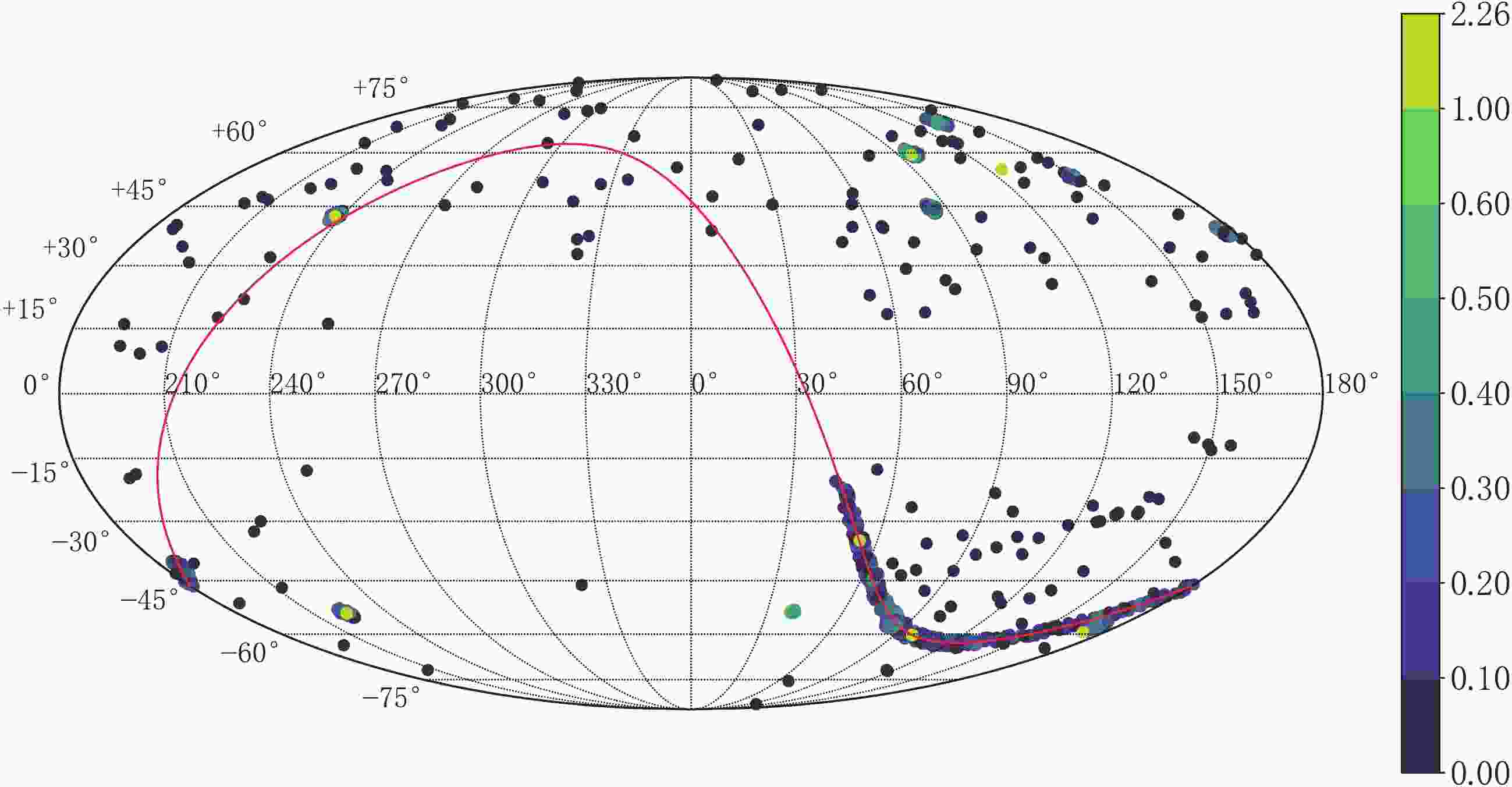
$ z $ , SDSS, SNLS and HST surveys. Compared to Union2 and the JLA sample, the number of SNe Ia in the Pantheon sample is enlarged and the systematic uncertainties are reduced by cross-calibration between subsamples. Fig. 1 shows the distribution of 1048 SNe Ia in the galactic coordinate system. As can be seen, the distribution of SNe Ia is inhomogeneous and half of them are located in the south-east of the galactic coordinate system. In particular, there are 335 SNe Ia that cluster in a narrow strip which corresponds to the equator in the equatorial coordinate system, and could have a significant impact on cosmic anisotropy.
Figure 1. (color online) The distribution of 1048 SNe Ia in the galactic coordinate system. The pseudo-colors indicate the redshift of these SNe Ia. The red solid curve represents the celestial equator.
In the Pantheon sample, the observed distance modulus is determined by a modified version of the Tripp formula [73],
$ \mu_{\rm o b s} = m_{B}-M+\alpha x_{1}-\beta c+\Delta_{M}+\Delta_{B}, $

(7) where
$ \mu_{\rm obs} $ denotes the observed distance modulus, and$ m_B $ and M are the apparent magnitude and the absolute magnitude of SNe Ia in the B-band, respectively.$ x_1 $ is the stretch parameter and c is the color parameter.$ \alpha $ represents the coefficient in the relation between luminosity and stretch.$ \beta $ represents the coefficient in the relation between luminosity and color.$ \Delta_M $ and$ \Delta_B $ are distance corrections that depend on the host galaxy mass of SNe Ia and the predicted bias from simulations, respectively. Since M is degenerate to$ H_0 $ , Scolnic et al. [62] gave a corrected apparent magnitudes, i.e.$ m_{\rm o b s} = \mu_{\rm o b s}+M $ . The theoretical apparent magnitude is given as$ m_{\rm t h} = \mu_{\rm t h}+M = 5 \log _{10} D_{L}+{\cal M}, $

(8) where
$ {\cal M} $ is a nuisance parameter, which depends on the Hubble constant$ H_0 $ and the absolute magnitude M.The dipole fitting method, proposed by Mariano & Perivolaropoulos [39], is widely used to investigate the anisotropy of the Universe. We consider the dipole modulation of the theoretical apparent magnitude in the isotropic ΛCDM , wCDM and CPL models, namely
$ \widetilde{m}_{\rm th} = m_{\rm th}[1+A_{\rm D}(\hat{{ n}} \cdot \hat{{ p}})], $

(9) where
$ A_{\rm D} $ indicates the dipole amplitude,$ \hat{{ n}} $ is the direction of the dipole, and$ \hat{{ p}} $ is the unit vector pointing to SNe Ia.$ {m}_{\rm th} $ indicates the theoretical apparent magnitude in the isotropic ΛCDM, wCDM and CPL models given by Eq. (8). In the galactic coordinate system, the direction of the dipole$ \hat{{ n}} $ can be parametrized as$ \hat{{ n}} = \cos(b)\cos(l)\hat{{ i}}+\cos(b)\sin(l)\hat{{ j}}+\sin(b)\hat{{ k}}, $

(10) where l is the galactic longitude and b is the galactic latitude.
$ \hat{{ i}} $ ,$ \hat{{ j}} $ and$ \hat{{ k}} $ are unit vectors along the axis in the Cartesian coordinates system. Similarly, the position of the ith SNe Ia can be parametrized as$ {\hat{{ p}}_{{ i}}} = \cos(b_i)\cos(l_i)\hat{{ i}}+\cos(b_i)\sin(l_i)\hat{{ j}}+\sin(b_i)\hat{{ k}}. $

(11) We can now compare the corrected apparent magnitudes
$ m_{\rm o b s} $ and the dipole-modulated theoretical apparent magnitude$ \widetilde{m}_{\rm th} $ , and constrain the parameters in the three dipole-modulated cosmological models. For the Finslerian cosmological model, the spacetime is intrinsically anisotropic and the dipole modulation is unnecessary, and the parameters are constrained by the comparison of$ m_{\rm o b s} $ and$ m_{\rm th} $ .To explore the whole cosmological parameter space, we employ the
$ \chi^2 $ statistics,$ \chi^2 = \Delta { \mu}^T \cdot { C}^{-1} \cdot \Delta { \mu} = \Delta { m}^T \cdot { C}^{-1} \cdot \Delta { m}, $

(12) where
$ \Delta { \mu} = { \mu}_{\rm obs}-{ \mu}_{\rm th} $ or$ \Delta { m} = { m}_{\rm obs}-{ m}_{\rm th} $ . The total covariance matrix takes the form$ { C} = { D}_{\rm stat}+{ C}_{\rm sys}, $

(13) where the diagonal matrix
$ { D}_{\rm stat} $ and the covariance matrix$ { C}_{\rm sys} $ denote the statistical uncertainties and the systematic uncertainties, respectively.Note added: The Pantheon supernovae data have been updated in the GitHub repository①.
$ z_{\rm cmb} $ has been corrected with the peculiar velocity correction for$ z<0.08 $ in the updated file lcparam_full_long_zhel.txt. The corrected apparent magnitude$ m_{\rm o b s} $ and its statistical uncertainties are also given in that file. The systematic uncertainties are given in the file sys_full_long.txt. In addition, the position of each SNe Ia can be found in the folder data_fitres. -
We use the MCMC method to explore the whole parameter space. Specifically, we use the affine-invariant MCMC ensemble sampler provided by emcee① [74], which is widely used in astrophysics and cosmology. In the dipole-modulated ΛCDM model, the fitting parameters are the matter density
$ \Omega_m $ , the nuisance parameter$ {\cal M} $ , the dipole amplitude$ A_D $ and the dipole direction (l, b). With respect to the dipole-modulated ΛCDM model, the dipole-modulated wCDM model has an extra parameter$ w_0 $ , and the dipole-modulated CPL model has two extra parameters,$ w_0 $ and$ w_1 $ . The Finslerian cosmological model formally has the same parameter space as the dipole-modulated ΛCDM model, but the dipole anisotropy is derived from the specific Finsler spacetime. In the MCMC method, the posterior distributions are determined by priors and the likelihood function, which is given as$ {\cal L} \propto \exp \left(-\chi^{2} / 2\right) $ . We use the flat prior for each parameter as follow:$\Omega_m\sim[0,1], $ ${\cal M}\sim[0,100], $ $ w_0\sim[-100,100], $ $w_1\sim[-100,100],\, A_{\rm D}\sim[0,1], $ $l\sim[-180^\circ,180^\circ],\;b\sim [-90^\circ,$ $ 90^\circ] $ .As mentioned above, we constrain the dipole anisotropy in four cosmological models, i.e. the dipole-modulated ΛCDM, wCDM and CPL models, and the Finslerian cosmological model, by using the Pantheon sample. The best fitting parameters can be obtained by maximizing the posterior. Our results are shown in Figs. 2-5 and summarized in Table 1. In Figs. 2-5, we show the marginalized posterior distribution for each cosmological model. In Table 1, we show the 95% confidence level (CL) upper limit of the dipole amplitude
$ A_{\rm D} $ , and the maximum and the 68% CL constraints① for the other parameters. Note that the galactic longitude has been converted to a positive value.
Figure 2. (color online) The 1-dimensional and 2-dimensional marginalized posterior distributions in the parameter space of the dipole-modulated ΛCDM model. The horizontal and vertical solid black lines mark the maximum of the 1-dimensional marginalized posteriors. The red line indicates the 95% CL upper limit of the dipole amplitude
$A_{\rm D}$ . l and b are in units of degrees.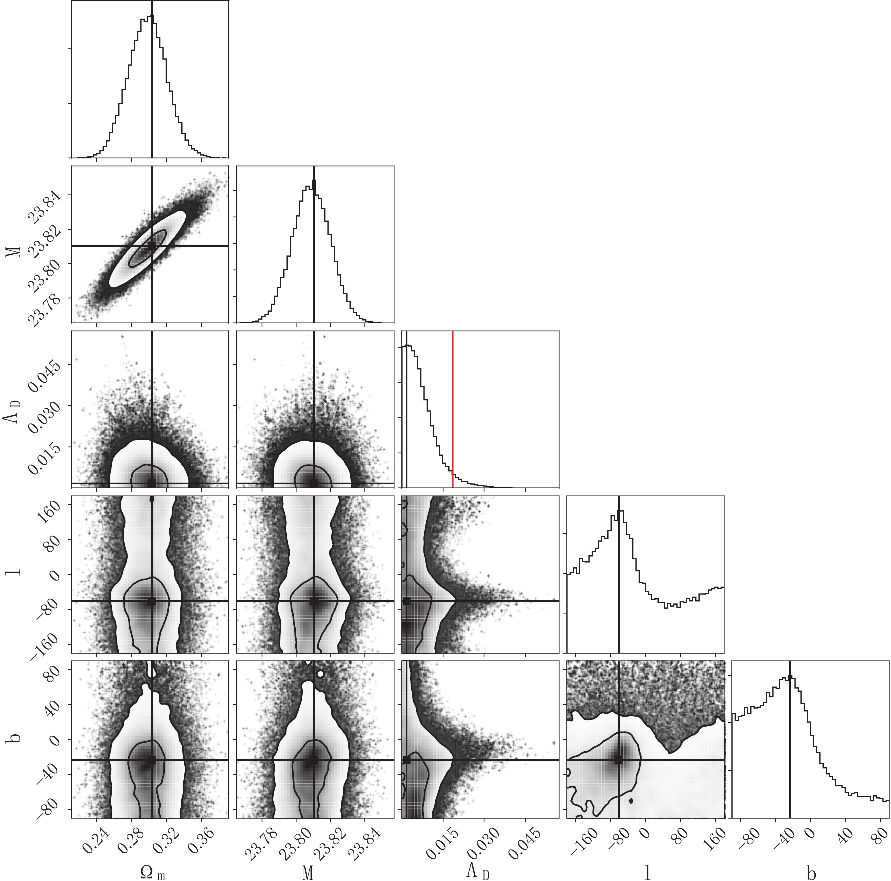
Figure 5. (color online) The 1-dimensional and 2-dimensional marginalized posterior distributions in the parameter space of the Finslerian cosmological model. The horizontal and vertical solid black lines mark the maximum of the 1-dimensional marginalized posteriors. The red line indicates the 95% CL upper limit of the dipole magnitude
$A_{\rm D}$ . l and b are in units of degrees.model $\Omega_m$ 

${\cal M}$ 

$w_0$ 

$w_1$ 

$A_{\rm D}(10^{-3})$ 

$l/(^{\circ})$ 

$b/(^{\circ})$ 

ΛCDM $ 0.303_{ -0.025}^{ +0.019}$ 

$ 23.809_{ -0.010}^{ +0.011}$ 

$-$ 

$-$ 

$<1.11$ 

$ 306.00_{ -125.98}^{ +91.94}$ 

$ -23.41_{ -54.71}^{ +22.97}$ 

wCDM $ 0.335_{ -0.082}^{ +0.066}$ 

$ 23.806_{ -0.014}^{ +0.016}$ 

$ -1.079_{ -0.162}^{ +0.271}$ 

$-$ 

$<1.14$ 

$ 298.81_{ -118.71}^{ +84.18}$ 

$ -19.80_{ -63.25}^{ +14.07}$ 

CPL $ 0.423_{ -0.141}^{ +0.060}$ 

$ 23.814_{ -0.020}^{ +0.018}$ 

$ -0.937_{ -0.215}^{ +0.218}$ 

$ 0.711_{ -3.633}^{ +0.959}$ 

$<1.09$ 

$ 313.20_{ -133.15}^{ +75.30}$ 

$ -27.00_{ -57.24}^{ +18.72}$ 

Finslerian $ 0.303_{ -0.027}^{ +0.017}$ 

$ 23.810_{ -0.013}^{ +0.009}$ 

$-$ 

$-$ 

$<18.50$ 

$ 298.80_{ -118.69}^{ +75.31}$ 

$ -23.41_{ -57.41}^{ +19.26}$ 

Table 1. The best fit values for the three dipole-modulated cosmological models and the Finslerian cosmological model. We show the maximum and the 68% CL constraints for the model parameters
$\Omega_m$ ,${\cal M}$ ,$w_0$ ,$w_1$ , l, b, and the 95% CL upper limits of the dipole amplitude$A_{\rm D}$ .
Figure 3. (color online) The 1-dimensional and 2-dimensional marginalized posterior distributions in the parameter space of the dipole-modulated wCDM model. The horizontal and vertical solid black lines mark the maximum of the 1-dimensional marginalized posteriors. The red line indicates the 95% CL upper limit of the dipole amplitude
$A_{\rm D}$ . l and b are in units of degrees.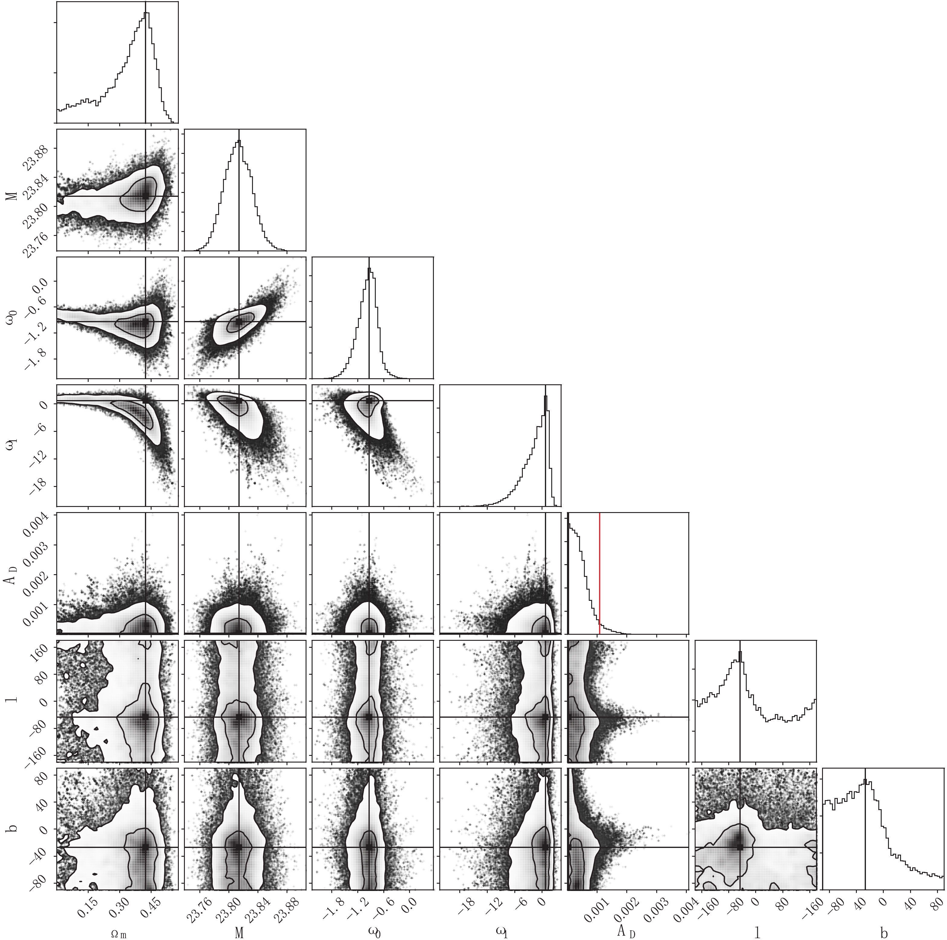
Figure 4. (color online) The 1-dimensional and 2-dimensional marginalized posterior distributions in the parameter space of the dipole-modulated CPL model. The horizontal and vertical solid black lines mark the maximum of the 1-dimensional marginalized posteriors. The red line indicates the 95% CL upper limit of the dipole amplitude
$A_{\rm D}$ . l and b are in units of degrees.In the dipole-modulated ΛCDM model, the matter density
$ \Omega_m $ and the nuisance parameter$ {\cal M} $ are well constrained by the Pantheon sample. The results are$\Omega_m = $ $ 0.303_{ -0.025}^{ +0.019} $ and$ {\cal M} = 23.809_{ -0.010}^{ +0.011} $ , which is in agreement with the results of Scolnic et al. [62], where they did not consider dipole anisotropy. In our case, we find that the dipole anisotropy is very weak, and the dipole amplitude is constrained as$ A_{\rm D} < 1.11\times 10^{-3} $ at 95% CL, while the dipole direction points towards$ (l,b) =({306.00^{\circ}}_{-125.98^{\circ}}^{+91.94^{\circ}},$ $ {-23.41^{\circ}}_{-54.71^{\circ}}^{+22.97^{\circ}}) $ . The very large uncertainty of the dipole direction implies that the dipole anisotropy in the dipole-modulated ΛCDM model is very weak.In the dipole-modulated wCDM model, the extra parameter, i.e. the equation of state of dark energy, is
$ w_0 = -1.079_{ -0.162}^{ +0.271} $ , which is also consistent with the results of Scolnic et al. [62]. The matter density is constrained as$ \Omega_m = 0.335_{ -0.082}^{ +0.066} $ and the nuisance parameter is constrained as$ {\cal M} = 23.806_{ -0.014}^{ +0.016} $ . Similarly to the dipole-modulated ΛCDM model, the dipole anisotropy is very weak and the dipole amplitude is constrained as$ A_{\rm D} < 1.14\times 10^{-3} $ at 95% CL. The dipole direction points towards$ (l,b) = ({ 298.81^{\circ}}_{-118.71^{\circ}}^{ +84.18^{\circ}},{-19.80^{\circ}}_{-63.25^{\circ}}^{+14.07^{\circ}}) $ , which is very close to the dipole direction in the dipole-modulated ΛCDM model.In the dipole-modulated CPL model, there are two extra parameters,
$ w_0 $ and$ w_1 $ , which are constrained as$ w_0 = -0.937_{ -0.215}^{ +0.218} $ and$ w_1 = 0.711_{ -3.633}^{ +0.959} $ . The matter density is$ \Omega_m = 0.423_{ -0.141}^{ +0.060} $ , which is slightly larger than in the dipole-modulated ΛCDM or wCDM models, and the nuisance parameter is$ {\cal M} = 23.814_{ -0.020}^{ +0.018} $ . The dipole amplitude is constrained as$ A_{\rm D} < 1.09\times 10^{-3} $ at 95% CL. The dipole direction points towards$ (l,b) = ({313.20^{\circ}}_{-133.15^{\circ}}^{+75.30^{\circ}}, $ ${-27.00^{\circ}}_{-57.24^{\circ}}^{+18.72^{\circ}}) $ , which is very close to the dipole directions mentioned above.In the Finslerian cosmological model, the matter density
$ \Omega_m $ and the nuisance parameter$ {\cal M} $ are constrained as$ \Omega_m = 0.303_{ -0.027}^{ +0.017} $ and$ {\cal M} = 23.810_{ -0.013}^{ +0.009} $ , which is almost the same as in the dipole-modulated ΛCDM model. The dipole anisotropy is very weak, and the dipole amplitude is constrained as$ A_{\rm D} < 18.50 \times 10^{-3} $ at 95% CL. The dipole direction points towards$ (l,b) = $ $ ({298.80^{\circ}}_{-118.69^{\circ}}^{+75.31^{\circ}}, $ $ {-23.41^{\circ}}_{-57.41^{\circ}}^{+19.26^{\circ}}) $ , which is very close to the dipole directions in the other three dipole-modulated cosmological models.Finally, we make a comparison between the dipole directions mentioned above in the Pantheon sample with those derived from the Union2 sample [39], Union2.1 sample [44] and JLA sample [50]. The dipole directions in each SNe Ia sample are shown in Fig. 6. As can be seen, the dipole directions in the four cosmological models are close to each other when using the Pantheon sample. The angular separation between these dipole directions are much smaller than their uncertainties. For the JLA sample, Lin et al. [50] arrived to almost the same conclusion, and they also considered the dipole-modulated ΛCDM, wCDM and CPL models. Interestingly, all dipole directions are close to the dipole direction in the Union2 and Union2.1 sample, within
$ 16.36^{\circ} $ , and their angular separation is much smaller than the uncertainty of the dipole direction. The star in Fig. 6 denotes the axial direction of the plane of the SDSS subsample in Pantheon, which points towards$ (l,b) = (302.93^{\circ}, -27.13^{\circ}) $ . As it turns out, the dipole directions in the Pantheon sample are very close to the axial direction of the plane of the SDSS subsample, and their angular separation is less than$ 9.14^{\circ} $ . Moreover, we find that the dipole directions shift more than$ 40.18^{\circ} $ when we exclude the SDSS subsample from Pantheon. This consistency confirms the conclusion that the SDSS subsample plays a dominant role in the dipole anisotropy in the Pantheon sample [65]. Similar conclusion was drawn for the Union2 sample [75]. Monte-Carlo simulations also showed that the anisotropic distribution of coordinates can lead to dipole directions and make the dipole magnitude larger [76]. Therefore, we suggest that the weak dipole anisotropy in the Pantheon sample originates from the inhomogeneous distribution of the SDSS subsample in Pantheon.
Figure 6. (color online) The dipole directions in four cosmological models using the Pantheon sample, and the dipole directions derived from the Union2 sample [39], Union2.1 sample [44] and JLA sample [50]. The star marks the axial direction of the plane of the SDSS subsample [65]. The uncertainties of dipole directions are given in Table 1.
-
The recently released Pantheon sample of SNe Ia was used to test the possible dipole anisotropy in the Finslerian cosmological model and the other three dipole-modulated cosmological models, i.e. the dipole-modulated ΛCDM, wCDM and CPL models. The MCMC method was used to explore the whole cosmological parameter space. We found that the dipole anisotropy is very weak in all cosmological models used. For the dipole-modulated ΛCDM model, the dipole amplitude has an upper limit of
$ 1.11 \times 10^{-3} $ at 95% CL , and the dipole direction points towards$ (l,b) = ({306.00^{\circ}}_{-125.98^{\circ}}^{+91.94^{\circ}},{-23.41^{\circ}}_{-54.71^{\circ}}^{+22.97^{\circ}}) $ . The dipole-modulated wCDM and CPL models have a similar dipole anisotropy. For the Finslerian cosmological model, the dipole amplitude has an upper limit of$ 18.50 \times 10^{-3} $ at 95% CL, and the dipole direction in the Finsler spacetime points towards$ (l,b) = ({298.80^{\circ}}_{-118.69^{\circ}}^{+75.31^{\circ}}, $ $ {-23.41^{\circ}}_{-57.41^{\circ}}^{+19.26^{\circ}}) $ . All these results show that the isotropic cosmological model is an excellent approximation. We also found that the dipole direction in Pantheon or the JLA sample is close to the dipole direction in the Union2 and Union2.1 samples. All dipole directions are close to the axial direction of the plane of the SDSS subsample in Pantheon. Therefore, we suggest that the weak dipole anisotropy in the Pantheon sample originates from the inhomogeneous distribution of the SDSS subsample. A more homogeneous distribution of SNe Ia is necessary to constrain the cosmic anisotropy.We thank Zhi-Chao Zhao for useful discussions. We greatly appreciate D. M. Scolnic for the private communication.
Constraining the anisotropy of the Universe with the Pantheon supernovae sample
- Received Date: 2019-09-24
- Available Online: 2019-12-01
Abstract: We test the possible dipole anisotropy of the Finslerian cosmological model and the other three dipole-modulated cosmological models, i.e. the dipole-modulated ΛCDM, wCDM and Chevallier–Polarski–Linder (CPL) models, by using the recently released Pantheon sample of SNe Ia. The Markov chain Monte Carlo (MCMC) method is used to explore the whole parameter space. We find that the dipole anisotropy is very weak in all cosmological models used. Although the dipole amplitudes of four cosmological models are consistent with zero within the


 DownLoad: