


 Abstract
 HTML
HTML Reference
 Related
 PDF
PDF


-
Charge exchange (CE) reactions, with hadronic probes such as (p, n), (3He, t), (12C, 12N), are used as one of the powerful tools for nuclear structure studies. The related interesting topics include the Gamow-Teller (GT) transitions in regions of excitation energy inaccessible to
$ \beta $ -decay [1–4], spin-dipole transitions [3], isovector giant monopole resonances [2, 5], symmetry energy [2, 6], isospin symmetry breaking force in asymmetric nuclear matter [6–8], the Gamow-Teller giant resonance and the Landau-Migdal parameter [8]. In particular, GT strengths are crucial for understanding various issues such as the late stellar evolution, neutrino nucleosynthesis and neutrinoless double$ \beta $ -decay [1, 3, 8]. It is known that heavy-ion probes allow a better extraction of the GT strength compared to the (p, n) reactions due to higher energy resolution, as well as stronger absorption at the surface of the target nucleus [1–4].Recently, more attention has been paid to the experimental studies of CE reactions at intermediate energies (
$ \geqslant $ $ 100$ MeV/nucleon) [2, 3, 8]. Systematic investigations indicate that the reaction mechanism at these energies is dominated by the one-step process, so that more precise extraction of the weak transition strengths, or of the nuclear structure information, can be obtained as long as the appropriate theoretical tools can be applied to describe the data [9]. However, few theoretical formulations and calculation tools exist for intermediate and high energies [4, 10, 11], although at lower energies (< 100 MeV/nucleon) the CE reactions have been successfully described by the conventional Distorted-Wave-Born-Approximation (DWBA) [12–16]. It is difficult to apply the DWBA method to CE reactions at intermediate energies since the required phenomenological potential is rarely available [4, 17]. Therefore, we try to follow the eikonal approximation, which can be formulated microscopically by using the nucleon densities and the bare nucleon-nucleon (NN) interaction [18]. As a first step, we follow the Normal Eikonal Approach (NEA) [18, 19], where the eikonal approximation is applied both to the relative motion and to the structural form factor. The results based on NEA show a considerable discrepancy compared with the conventional DWBA calculations for CE reactions at$ 140$ MeV/nucleon. It was found that this is caused by the approximate treatment of the form factor, which carries the sensitive nuclear structure information. As the second step, we develop the Improved Eikonal Approach (IEA), in which the eikonal (straight-line) approximation is still applied to the relative motion, while it is removed from the structural part, so that the form factor remains a strict three-dimensional function in coordinate space. Based on IEA, the calculated differential cross-sections (DCS) are in good agreement with the conventional DWBA calculations and with the experimental results for CE reactions at$ 140$ MeV/nucleon. -
The DCS for the CE reaction A(a, b)B is usually expressed as [17, 20]:
$ \frac{\rm{d}\sigma}{\rm{d}\Omega}(\theta) = \frac{1}{(2J_{\rm A}+1)(2J_{\rm a}+1)}\sum\limits_{\substack{M_{\rm a}M_{\rm b}\\M_{\rm A}M_{\rm B}}} \big|f(\theta)\big|^{2}, $

(1) where
$ J_{\rm i} $ and$ M_{\rm i} $ are the spin and magnetic quantum number of the particle i (i$ \, $ =$ \, $ a, b, A and B), respectively. At intermediate energies, the difference between the amplitudes of the initial and final momentum can be neglected, and thus the scattering amplitude$ f(\theta) $ in DWBA approach can be defined in terms of the interaction matrix element [17, 20]:$ f(\theta) = \frac{-\mu}{2\pi\hbar^{2}}\langle\chi^{(-)}_{{{k}}'}({{R}})\Phi_{\rm b}\Phi_{\rm B}\mid V\mid\Phi_{\rm a}\Phi_{\rm A}\chi^{(+)}_{{k}}({{R}})\rangle, $

(2) where
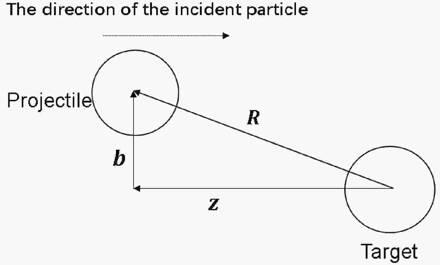
$ \mu $ is the reduced mass of the reaction system,$ \chi^{(\pm)}({{R}}) $ the incoming (+)/outgoing (-) distorted wave function,$ {{k}}({{{k}}'}) $ the initial (final) relative momentum, and$ {{R}} $ the vector of the relative position between a and A, or b and B, as seen in Fig. 1 and Fig. 3. In Eq. (2),$ \Phi $ is the internal wave function of the corresponding nucleus, and V the effective interaction potential which results in the charge exchange.
Figure 1. Schematic of the coordinate system used in the text.
In the eikonal approximation, which is valid at relatively high incident energies, the incoming distorted wave
$ \chi_{{k}}^{(+)} $ is assumed to have the form [17, 20]:$ \chi_{{k}}^{(+)}({{R}}) = {\rm e}^{{\rm i}kz} {\rm e}^{{\rm i}\chi({{R}})}, $

(3) where the z axis is parallel to the direction of the incident particles. The outgoing distorted wave
$ \chi^{(-)}_{{{k}}^{\prime}} $ is the time reversal of$ \chi_{{{k}}^{\prime}}^{(+)} $ . In Eq. (3),$ {\rm e}^{{\rm i} kz} $ with large k is a rapidly oscillating plane wave along the z axis, while$ {\rm e}^{{\rm i}\chi({{R}})} $ is characterized by the relatively slow oscillation. Here, one usually adopts the cylindrical coordinates so that$ {{R}} $ can be replaced by$ {{b}}+z{{{e}}_{{z}}} $ as shown in Fig. 1. The vector in the plane perpendicular to the z axis,$ {{b}} $ , is usually called the impact parameter.Again, according to the eikonal approximation, the phase shift function
$ \chi({{R}}) $ in Eq. (3) can be replaced by the two dimensional function$ \chi({{b}}) $ [17, 19, 20]:$ \chi({{b}})= -\frac{\mu}{\hbar^{2} k}\int^{+\infty}_{-\infty}U({{b}},z)\,{\rm d}z, $

(4) where U is the overall interaction potential between the initial particles a and A, or the final particles b and B. The product
$ \chi^{(-)\star}_{{{k}}'}\cdot\chi^{(+)}_{{k}} $ in the expression of$ f(\theta) $ is then${\rm e}^{-{\rm i}{{q}}\cdot{{R}}}{\rm e}^{{\rm i}\chi({{b}})} $ [19]. Here,$ {{q}} $ , the transferred momentum, is equal to$ {{{k}}'}-{{k}} $ $ \, $ , as illustrated in Fig. 2, with$ q\,\approx\,2k\sin\dfrac{\theta}{2} $ at relatively high energies.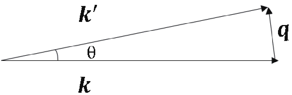
Figure 2. Schematic definition of the scattering angle
$\theta$ , the angle between the final momentum${{{k}}'}$ and the initial momentum${{k}}$ .${{q}}$ is the transferred momentum.Generally, the potential U in Eq. (4) includes the nuclear and Coulomb parts. Correspondingly,
$ \chi({{b}}) $ is also the sum of$ \chi_{\rm{N}} $ and$ \chi_{\rm{C}} $ , the nuclear and Coulomb phase shift functions.In order to make a direct comparison with the results of DWBA calculations, we may simply take U as the phenomenological optical potential (OP), and use it in both the CEX and DWBA codes. In case the phenomenological potential U, alternatively, is unavailable, a microscopic method, called the “
$ t_{\rho\rho} $ ” method, can be adopted to calculate$ \chi_{\rm{N}} $ :$ \chi_{\rm{N}}(b) = \int^{\infty}_{0} {\rm d}q\, q \rho_{\rm{p}}(q)\rho_{\rm{t}}(q)f_{\rm{NN}}(q)J_{0}(qb), $

(5) where
$ f_{\rm{NN}} $ is the NN scattering amplitude, and$ \rho_{\rm{p}} $ and$ \rho_{\rm{t}} $ the nucleon densities of the projectile and target. Using this method, the application of the eikonal approximation can be extended to higher incident energies ($ E\, $ up to$ \sim 1\,\rm{GeV} $ ), where the phenomenological potential U is rarely available [11].Based on the eikonal approximation,
$ f(\theta) $ in Eq. (2) becomes:$ f(\theta) = \frac{-\mu}{2\pi\hbar^{2}}\int {\rm d}{{R}}\,{\rm e}^{-{\rm i}{{q}}\cdot{{R}}}\,{\rm e}^{{\rm i}\chi{({{b}})}}F({{R}}). $

(6) Here,
$ F({{R}}) $ , the form factor carrying the nuclear structure information, is defined by:$ F({{R}}) = \langle J_{\rm{B}}T_{\rm{B}}J_{\rm{b}}T_{\rm{b}} \mid V \mid J_{\rm{A}}T_{\rm{A}}J_{\rm{a}}T_{\rm{a}} \rangle, $

(7) where
$ T_{{\rm i}} $ is the isospin of the nucleus i (i$ \, $ =$ \, $ a, b, A and B). V in Eq. (7) is the residual interaction between the valence nucleons, which is responsible for the CE reaction. More specifically, V is given by [19]:$\begin{split} {V = \sum\limits_{{\rm t}_{i}{\rm p}_{j}}\,V_{{\rm t}_{i}{\rm p}_{j}}} =&{ \sum\limits_{{\rm t}_{i}{\rm p}_{j}}\sum\limits_{s_{0}t_{0}K}\,A^{K}_{s_{0}}\,V^{K}_{s_{0}t_{0}}(r_{{\rm t}_{i}{\rm p}_{j}}) (\tau^{t_{0}}_{1}\cdot\tau^{t_{0}}_{2})}\\ &{\times[Y_{K}(\widehat {{{{r}}_{{{\bf{t}}_{{i}}}{{\bf{p}}_{{j}}}}}})\cdot(\sigma^{s_{0}}_{1}\otimes\sigma^{s_{0}}_{2})^{K}],} \end{split} $

(8) where
${{r_{{\rm t}_i {\rm p}_j}}}$ is the spatial coordinate between the interacting target nucleons “${\rm t}_{i} $ ” and projectile nucleons “$ {\rm p}_{j}$ ” , as indicated in Fig. 3. Here,$ s_{0} $ , the change of spin of the interacting nucleons, has two values, 1 and 0, corresponding to the spin-flip and non-spin-flip processes, respectively. The change of isospin,$ t_{0} $ , is 1 for CE reactions. In Eq. (8),$ K\, = \,0 $ and$ K\, = \,2 $ correspond to the central and tensor forces, respectively. The constants$ A^{K}_{s_{0}} $ have the values$ \sqrt{4\pi} $ ,$ -\sqrt{12\pi} $ and$ \sqrt{4\pi/5} $ , for$ A^{0}_{0} $ ,$ A^{0}_{1} $ and$ A^{2}_{1} $ , respectively [19]. In Eq. (8), the NN interaction strength functions$ V^{K}_{s_{0}t_{0}}(r) $ include both the central (K = 0) and the tensor (K = 2) parts. Their parameters are taken from [21, 22]. Given the exchange and medium effects, the modified NN interaction strength functions are given in [21], which were adopted in the present work.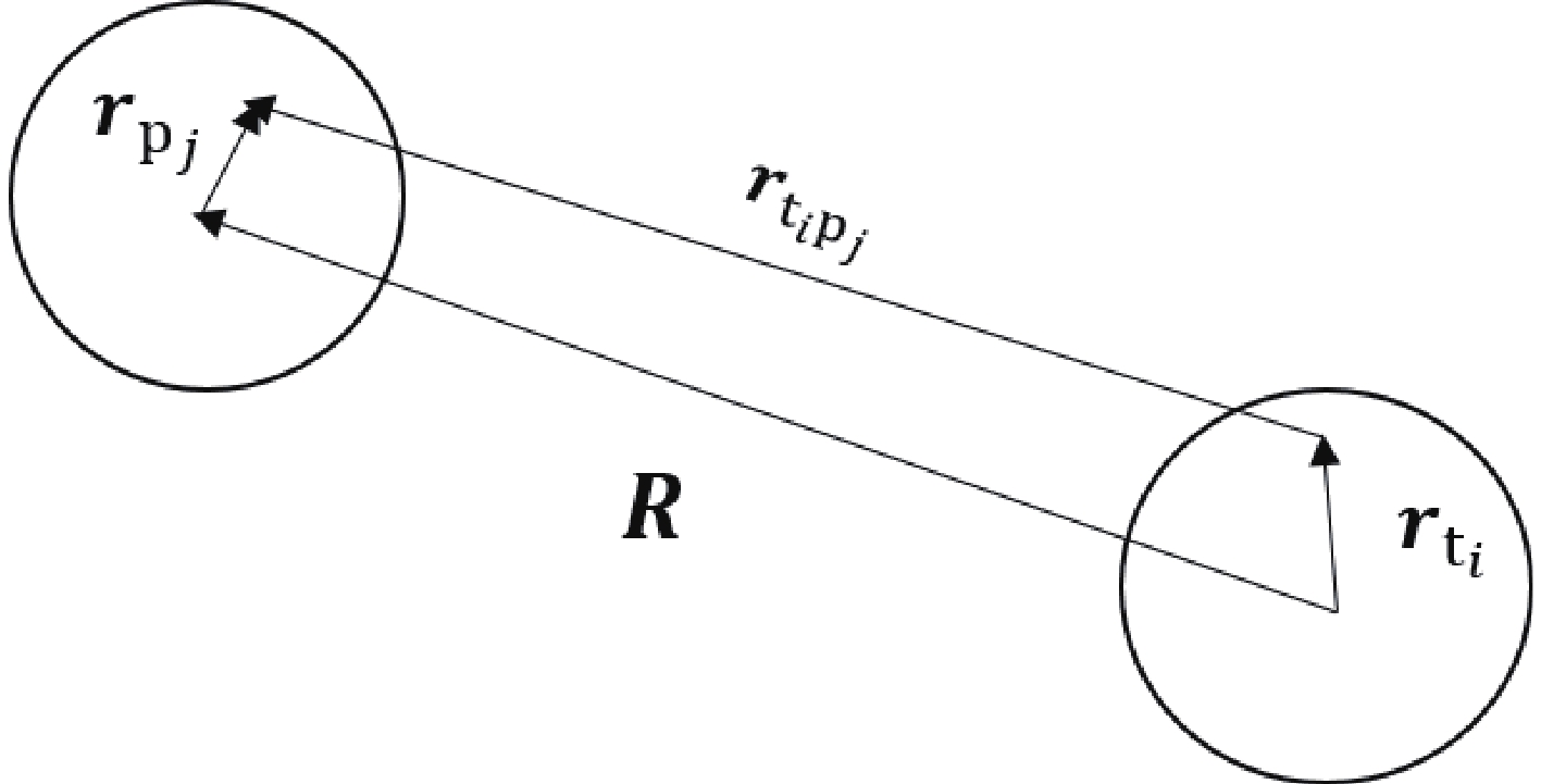
Figure 3. The coordinates used in the text.
$R$ is the distance between the center-of-mass of the nuclei, and$r_{{\rm p}_{j}}$ /$r_{{\rm t}_{i}}$ the distance between the interacting nucleons${\rm p}_{j}$ /${\rm t}_{i}$ and the center-of-mass of the projectile/target.Combining Eq. (8) with Eq. (7),
$ F({{R}}) $ can be decomposed into the partial form factor$ F^{JSL_{{\rm tr}}} ({{R}}) $ weighted by the C-G coefficients:$\begin{split} F({{R}}) =&{ \sum\limits_{\substack{J,S,L_{\rm{tr}}\\M_{\rm{tr}}M_{J}M_{S}}}C^{J_{{B}}M_{{B}}}_{J_{{A}}M_{{A}}JM_{J}}C^{J_{{b}}M_{{b}}}_{J_{{a}}M_{{a}}SM_{S}}}\\ &{\times C^{L_{{\rm tr}}M_{\rm{tr}}}_{SM_{S}JM_{J}}F^{JSL_{{\rm tr}}} ({{R}}), } \end{split} $

(9) where
$ J/S $ is the total spin transferred to the intrinsic motion of the target/projectile system,$ L_{\rm{tr}} $ the total transferred angular momentum, and$ M_{\rm{tr}} $ the associated magnetic quantum number. It is natural that the partial form factor (matrix element)$ F^{JSL_{{\rm tr}}}({R}) $ requires the states and wave functions of the interacting (valence) nucleons as input. One possibility is to use the One Body Transition Densities (OBTD), including the configuration mixing, which can be obtained from the shell model calculations using for instance the OXBASH code [1, 23]. The exact expressions for OBTD, together with the corresponding single-particle wave functions, can be found in [12–15, 24, 25]. The detailed expressions for OBTD are beyond the scope of this article and, hence, are omitted.For simplicity, the numerical calculations are performed in momentum space. Therefore,
$ F({{R}}) $ is expressed by the inverse Fourier transformation of the form factor in the momentum space$ F({{p}}) $ :$ F({{R}}) = \int {\rm d}{{p}}\,{\rm e}^{-{\rm i}{{p}}\cdot{{R}}}F({{p}}). $

(10) Inserting Eq. (10) into Eq. (6),
$ f(\theta) $ becomes:$ \begin{split} f(\theta)= &{-\frac{\mu}{2\pi\hbar^{2}} \int {\rm d}{{b}}\,{\rm d}z\,{\rm e}^{-{\rm i}{{q}}\cdot{{R}}}{\rm e}^{{\rm i}\chi({{b}})}}\\ &{\times\int{\rm d}{{p}}\,{\rm e}^{-{\rm i}{{p}}\cdot{{R}}}F({{p}}).} \end{split} $

(11) According to NEA, the integral over z on
$ {\rm e}^{-{\rm i}({{q}}+{{p}})\cdot{{R}}} $ in Eq. (11) is performed and yields a delta function$ \delta(q_{{\rm z}}+p_{{\rm z}}) $ . Further, by using$ q_{{\rm z}}\,\approx\,0 $ , Eq. (11) in this approach becomes:$ \begin{split} f^{{\rm NEA}}(\theta) =&{ -\frac{\mu}{\hbar^{2}} \int {\rm d}{{b}}\,{\rm e}^{-{\rm i}{{q}}\cdot{{b}}} {\rm e}^{{\rm i} \chi({{b}})}}\\ &{\times\int{\rm d}{{p}}_{\perp}\,{\rm e}^{-{\rm i}{{p}}_{\perp}\cdot{{b}}} F({{p}}_{\perp}),} \end{split}$

(12) where
$ {{p}}_{\perp} $ is a two-dimensional momentum in the plane perpendicular to the z axis. In this way,$ F({{R}}) $ is reduced to a two-dimensional function$F^{{\rm NEA}}({{b}}) = $ $ \int{\rm d}{{p}}_{\perp}\,{\rm e}^{-{\rm i}{{p}}_{\perp}\cdot{{b}}} F({{p}}_{\perp}) $ .For comparison, in IEA
$ q_{{\rm z}}\,\approx\,0 $ is directly used in${\rm e}^{-{\rm i}{{q}}\cdot{{R}}} $ , so that${\rm e}^{-{\rm i}{{q}}\cdot{{R}}} $ is replaced by$ {\rm e}^{-{\rm i}{{q}}\cdot{{b}}} $ and Eq. (11) becomes:$ \begin{split} f^{{\rm IEA}}(\theta) =&{ -\frac{\mu}{2\pi\hbar^{2}} \int {\rm d}{{b}}\,{\rm d}z\,{\rm e}^{-{\rm i}{{q}}\cdot{{b}}} {\rm e}^{{\rm i}\chi({{b}})} }\\ &{\times\int{\rm d}{{p}}\,{\rm e}^{-{\rm i}{{p}}\cdot{{R}}}F({{p}}) . } \end{split} $

(13) One can see that the form factor
$ F({{R}}) $ in IEA is a three-dimensional function. In other words,$F^{{\rm IEA}}({{R}})\!= $ $ \!\int {\rm d}{{p}}{\rm e}^{-{\rm i}{{p}}\cdot{{R}}}F({{p}}) $ .The term
$ {\rm e}^{-{\rm i}{{p}}\cdot{{R}}} $ above can be expanded into a series of three-dimensional partial terms:$ {\rm e}^{-{\rm i}{{p}}\cdot{{R}}} = 4\pi\sum\limits_{LM}i^{-L}j_{L}(pR)Y_{LM}(\hat{{{p}}})Y^{\ast}_{LM}(\hat{{{R}}}), $

(14) Correspondingly, DCS for CE reactions (Eq. (1)) can be decomposed in the form:
$ \frac{\rm{d}\sigma}{\rm{d}\Omega}(\theta) = \frac{\mu^{2}}{\hbar^{4}}\frac{(2J_{{B}}+1)(2J_{{b}}+1)}{(2J_{{A}}+1)(2J_{{a}}+1)}\sum\limits_{\substack{JSL_{{\rm tr}}\\M_{\rm{tr}}}} \big|\beta(\theta)\big|^{2}. $

(15) The detailed expression for the partial amplitude
$ \beta(\theta) $ can be easily deduced for NEA or IEA using the above derivations.Apart from CE reactions, the eikonal approximation can also be applied to the elastic scattering cross-section. DCS for elastic scattering can be written as [11, 19]:
$ \frac{{\rm d}\sigma}{{\rm d}\Omega}(\theta) = \big|f_{\rm{el}}(\theta)\big|^{2}, $

where the elastic scattering amplitude,
$ f_{{\rm el}}(\theta) $ , is defined by [11]:$ f_{{\rm el}}(\theta) =-\frac{1}{4\pi}\int {\rm e}^{-{\rm i}{{{k}}'}\cdot{{R}}}U({{R}})\psi^{\prime}({{R}}){\rm d}{{R}}. $

(16) In the eikonal approximation,
$ f_{{\rm el}}(\theta) $ becomes [11]:$ \begin{split} f_{{\rm el}}(\theta) = &{f_{\rm{C}}(\theta)+ik\int_{0}^{\infty}{\rm d}b\, b J_{0}(qb) {\rm e}^{[{\rm i}\chi_{{\rm C}}(b)]}}\\ &{\times[1-{\rm e}^{{\rm i}\chi_{{\rm N}}(b)}], } \end{split}$

where
$ f_{{\rm C}}(\theta) $ is the scattering amplitude given by the point-charge Coulomb potential [20]. -
Before presenting a comprehensive treatment of CE reactions, we start with a test of the coding technique by evaluating a simple case, elastic scattering with the eikonal approximation. As demonstrated in Fig. 4, the results are in perfect agreement with the conventional Optical Model (OM) calculations [26], for scattering at
$ 140$ MeV/nucleon and at small angles ($ \theta< 20 $ deg). Some divergence appears at larger angles, which is reasonable since the eikonal approximation is valid only for small scattering angles and at relatively high energies [11, 17, 20]. It should be noted that, for a direct comparison, the same OP parameters from [1, 25] are used in both the eikonal approximation and the OM calculations.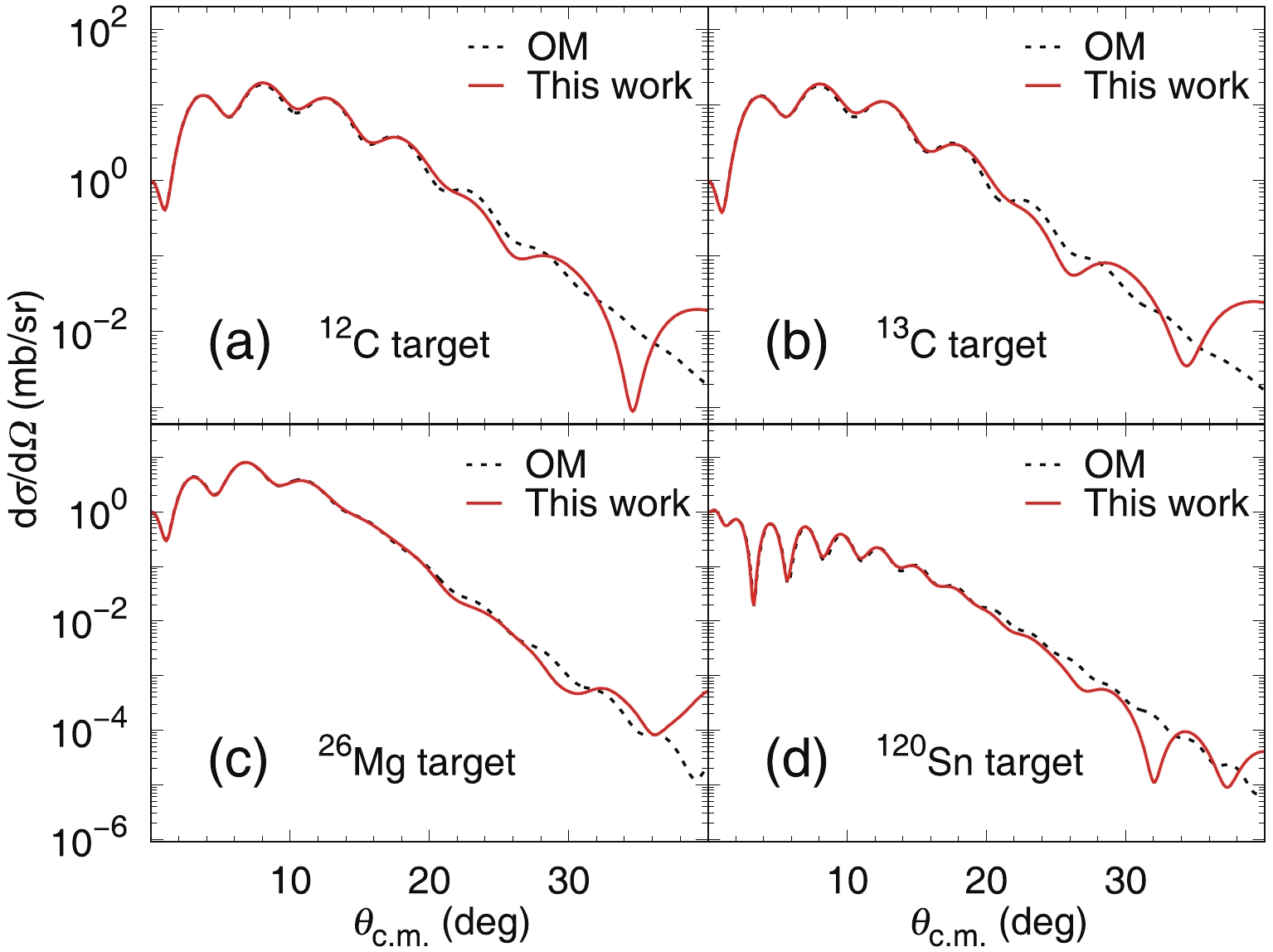
Figure 4. (color online) Comparison of the elastic scattering DCS between our calculations (red-solid lines) and the OM calculations (black-dashed lines). (a), (b), (c) and (d) correspond to the elastic scattering of 3He at 140 MeV/nucleon on 13C, 12C, 120Sn and 26Mg targets, respectively.
For CE reactions, we first perform calculations of DCS in NEA. According to Eq. (15), DCS for CE reactions is determined by all possible and independent
$ JSL_{{\rm tr}}\,-\, $ components. For GT-type CE reactions, they are 110- ($ J = 1,\,S = 1,\,L_{{\rm tr}} = 0 $ ) and 112- components. As can be seen in Fig. 5, the results show considerable discrepancy between the NEA calculations and the conventional DWBA calculations (FOLD program) for the 112- component and the total DCS, although a good agreement for the 110- component is obtained (not shown). Three GT-type CE reactions, all at$ 140$ MeV/nucleon, are checked: 12C (3He, t) 12N, 26Mg (3He, t) 26Al and 120Sn (3He, t) 120Sb. We note again that all input parameters are the same for both calculations, including the overall optical potential U, the residual NN interaction potential V and OBTD [1, 21, 22, 25]. Therefore, the difference between the calculated results is related to the approximations of the models.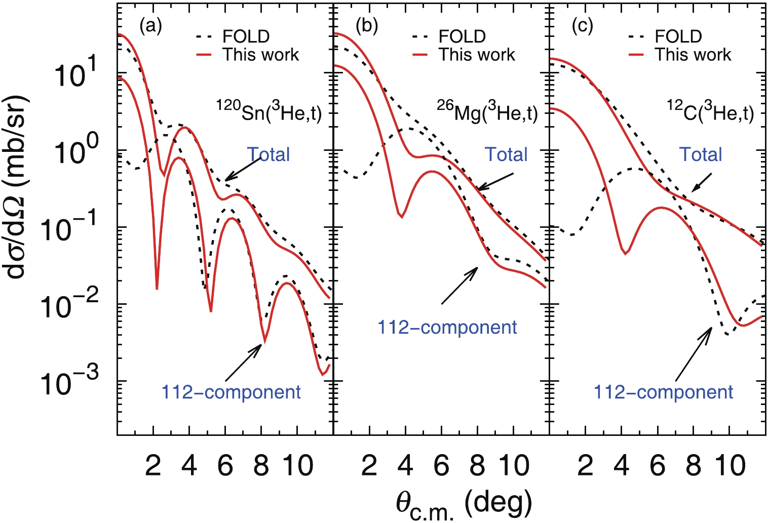
Figure 5. (color online) Comparison between the DWBA (black-dashed lines) and NEA (red-solid lines) calculations for the 112- component and the total DCS. Three GT-type CE reactions, all at 140 MeV/nucleon, are used: (a) 120Sn (3He, t) 120Sb; (b) 26Mg (3He, t) 26Al and (c) 12C (3He, t) 12N.
Thereafter, the calculations are performed based on the new approach, IEA. As shown in Fig. 6, two calculations, again using exactly the same input parameters, are in perfect agreement for both the 112- component and the total DCS, for the three GT-type reactions at
$ 140$ MeV/nucleon. The difference between NEA and IEA for the 112- component can be further understood by looking at the contributions related to each quantum number. As indicated above (Eq. (9)), the 112- component implies$ L_{\rm tr} = 2 $ and$ M_{\rm tr} $ =$ 0, \pm 2 $ (only even numbers are effective). It is found that when applying the eikonal approximation to the form factor, such as in NEA, the important contributions from the$ M_{\rm tr} $ = ±2 terms vanish automatically. By using the strict three-dimensional form factor, such as in IEA, these terms are recovered and good results can be obtained. This finding is in line with the physics meaning of each term, according to the kinematic picture. Since only the$ M_{\rm tr} $ =$ 0 $ term is allowed for the 110- component, it does not show any difference between the NEA and IEA calculations. It is clear that the IEA treatment is crucial for the applicability of the eikonal approximation to CE reactions at intermediate energies.
Figure 6. (color online) Comparison between the calculations using the DWBA approach (black-dashed lines) and IEA (red-solid lines), for the 112- component and the total DCS. The reactions used are the same as in Fig. 5.
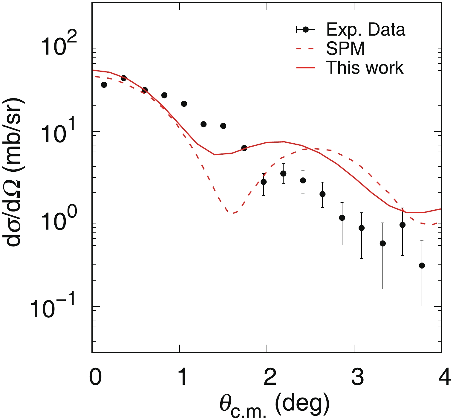
We also tried to apply IEA to the experimental data for a mirror reaction 13C (13N,13C) 13N at
$ 105 $ MeV/nucleon [27]. Here,$ V^{K}_{s_{0}t_{0}}(r) $ at$ 105 $ MeV/nucleon is deduced by interpolation of the potentials at 50, 100, 140, 175, 210, 270, 325, 425, 515, 650, 725, 800 and$ 1000 $ MeV/nucleon [21, 22]. The OP parameters are obtained from [28]. OBTD are obtained using the OXBASH code with pwt interaction [29] in the p-shell space. As shown in Fig. 7, the IEA calculations are comparable with the experimental results and with the results obtained using the single-particle model (SPM) [28]. It is worth noting that the experimental angular distribution has no oscillatory structure due to the very limited angular resolution of the detection system [27]. What is important here is the correct reproduction of the cross-section at 0 degrees, from which the GT transition strength can be extracted [1, 30]. The actual IEA predictions of$ \dfrac{{\rm d}\sigma}{{\rm d}\Omega}(0^{\circ}_{{\rm c.m.}}) $ are respectively 50.43 mb/sr and 64.73 mb/sr, for the pwt [29] and ckpot interactions [31] in the shell-model calculations. Both agree with the present experimental value of 56$ \pm $ 10 mb/sr [27] within the error bar. -
In order to describe CE reactions at intermediate energies, we first tried to implement the NEA formulation. Test calculations for CE reactions at 140 MeV/nucleon showed considerable discrepancy with respect to the conventional DWBA calculations. Thereafter, the formulation was improved (IEA) by removing the influence of the eikonal approximation from the form factor so as to keep it a strict three-dimensional function. Calculations based on IEA are in good agreement with DWBA calculations for various CE reactions at 140 MeV/nucleon, and with the experimental data at 105 MeV/nucleon. Since the eikonal approximation can be easily formulated in a microscopic way, relying only on the nuclear matter density distribution and the bare nucleon-nucleon interaction (see Eq. (5)), it has the obvious advantage when applied to CE reactions at higher energies, where the phenomenological OP, required for DWBA, is rarely available. Based on the current benchmark test, the IEA approach is ready to be compared to the experimental data, and to be applied to the extraction of the related physics quantities, although some improvements could further be made for relativistic energies.
We would like to thank Prof. C.A. Bertulani for the initial ideas and useful discussions of the theoretical description of CE reaction at intermediate energies. He also provided part of the NEA formulas.
Improved eikonal approach for charge exchange reactions at intermediate energies
- Received Date: 2019-07-28
- Available Online: 2019-12-01
Abstract: In order to describe charge exchange reactions at intermediate energies, we implemented as a first step the formulation of the normal eikonal approach. The calculated differential cross-sections based on this approach deviated significantly from the conventional DWBA calculations for CE reactions at 140 MeV/nucleon. Thereafter, improvements were made in the application of the eikonal approximation so as to keep a strict three-dimensional form factor. The results obtained with the improved eikonal approach are in good agreement with the DWBA calculations and with the experimental data. Since the improved eikonal approach can be formulated in a microscopic way, it is easy to apply to CE reactions at higher energies, where the phenomenological DWBA is a priori difficult to use due to the lack, in most cases, of the required phenomenological potentials.


 DownLoad: