Note on single-trace EYM amplitudes with MHV configuration

I. INTRODUCTION

• I. INTRODUCTION
• II. BACKGROUND
•      A Spinor-helicity formalism in four dimensions
•      B SBDW and spanning forest formulae
• III. AMPLITUDES WITH THREE GRAVITONS
• IV. GENERAL FORMULA
• V. CONCLUSIONS

In four dimensional spacetime, tree-level single-trace maximally-helicity-violating (MHV) amplitudes within the Einstein-Yang-Mills (EYM) theory have been shown to satisfy the Selivanov-Bern-De Freitas-Wong (SBDW) formula [1−3], which expresses the amplitude through a generating function. The Cachazo-He-Yuan (CHY) [4−6] formula provides a general approach to EYM amplitudes that is independent of the spacetime dimensions and helicity configuration. In four dimensions, the CHY formula has been shown to provide a spanning forest formula (first proposed for gravity, following the lines of [7], [8], and [9]) for single-trace MHV amplitudes [10], which was further proven to be equivalent to the SBDW formula [10] and generalized to double-trace MHV amplitudes [11] through a recursion expansion formula [12−16].

From another perspective, as pointed out in earlier literature [17−21], each graviton in an EYM amplitude could be considered as a pair of collinear gluons carrying the same momentum and helicity. In particular, inspired by the SBDW formula, it was pointed out in [18] that single-trace MHV amplitudes with one or two gravitons can be explicitly expressed in terms of MHV amplitudes in which each graviton splits into a pair of collinear gluons [18]. This explicit formula for single-trace MHV amplitudes has not yet been extended to cases with an arbitrary number of gravitons. On this note, we take a small step forward in this direction by providing a general formula for single-trace MHV amplitudes in which each graviton splits into a pair of collinear gluons. When the number of gravitons is one or two, this formula reduces to the known results [18]. We expect that this approach provides new insights into the study of helicity amplitudes within the EYM theory.

This note is organized as follows. In Section II, we present a helpful review of the spinor-helicity formalism and SBDW formula. We study the amplitude with three gravitons in Section III and outline the general proof in Section IV. Further discussion and conclusions are presented in Section V.

II. BACKGROUND

• I. INTRODUCTION
• II. BACKGROUND
•      A Spinor-helicity formalism in four dimensions
•      B SBDW and spanning forest formulae
• III. AMPLITUDES WITH THREE GRAVITONS
• IV. GENERAL FORMULA
• V. CONCLUSIONS

In this section, we briefly review the spinor-helicity formalism in four dimensions [22] as well as the SBDW [1−3] and spanning forest [10] formulae for single-trace EYM amplitudes.

A Spinor-helicity formalism in four dimensions

• I. INTRODUCTION
• II. BACKGROUND
•      A Spinor-helicity formalism in four dimensions
•      B SBDW and spanning forest formulae
• III. AMPLITUDES WITH THREE GRAVITONS
• IV. GENERAL FORMULA
• V. CONCLUSIONS

The momentum $k^{\mu}_i$of each on-shell massless particle i is expressed by two copies of Weyl spinors, namely $\lambda_i^{a}\widetilde{\lambda}_i^{\dot{a}}$. We define the spinor products as

where $\epsilon_{{a}{b}}$ and $\epsilon_{\dot{a}\dot{b}}$ are totally antisymmetric tensors. The spinor products seem to be antisymmetric objects under the exchange of both spinors. With this expression, the Lorentz contraction of two momenta $k^{\mu}_a$ and $k^{\mu}_b$ reads

Additional helpful properties within the spinor-helicity formalism are as follows:

● Momentum conservation for an n-point amplitude:

● Schouten identity:

● Eikonal identity resulting from Schouten identity:

Finally, the n-gluon MHV amplitude $A(1,2,\cdots,n)$ at tree level satisfies the famous Parke-Taylor formula [23] ¹:

where i and j denote two negative-helicity gluons, and other gluons are supposed to be positive-helicity ones.

B SBDW and spanning forest formulae

• I. INTRODUCTION
• II. BACKGROUND
•      A Spinor-helicity formalism in four dimensions
•      B SBDW and spanning forest formulae
• III. AMPLITUDES WITH THREE GRAVITONS
• IV. GENERAL FORMULA
• V. CONCLUSIONS

Within the EYM theory, there are two possible configurations for tree-level single-trace MHV amplitudes, namely ($g^-,g^-$) and ($h^-,g^-$), which correspond to amplitudes with two negative-helicity gluons and one negative-helicity gluon plus one negative-helicity graviton, respectively. In the following, we focus on the ($g^-,g^-$) configuration; ($h^-,g^-$) can be studied similarly.

The SBDW formula [1−3] expresses the single trace ($g^-g^-$)-MHV amplitude $A(1,2,\cdots,i,\cdots,j,\cdots,N|\mathrm{H})$within the EYM theory as follows:

where $1,2,\cdots,N$ are gluons arranged in a fixed ordering, and$\mathrm{H} = \{n_1,n_2,\cdots,n_M\}$ are gravitons that are independent of color orderings. The negative-helicity gluons are supposed to be i and j. The $S(i,j,\mathrm{H},\{1,2,\cdots,N\})$ factor is generated by an exponential generating function, specifically

where

where $\xi$, $\eta$ are arbitrarily chosen reference spinors and G is the gluon set. In this note, we set $\xi = 1$ and $\eta = N$to study the ($g^-,g^-$) configuration.

It was shown in [10] that $S(\mathrm{H};\mathrm{G})$can be expanded using the spanning forest form. In particular,

where we have summed over all possible forests F, gluons and gravitons are considered as vertices, and gluons are considered as the root set. Each edge $ab$ is dressed by $\psi_{ab}$, and all such edges are multiplied in a given forest F.

In the case of ($h^-,g^-$), Eqs. (2), (3), and (5) slightly change as follows [3, 10, 11]: (i)$i,j$ are replaced in Eq. (2) by the negative helicity graviton and negative-helicity gluon; (ii) the graviton set H is replaced in Eqs. (3) and (5) by the positive-helicity graviton set $\mathrm{H}^+$, while the root set remains the gluon set; (iii) an extra $(-1)$is introduced.

III. AMPLITUDES WITH THREE GRAVITONS

• I. INTRODUCTION
• II. BACKGROUND
•      A Spinor-helicity formalism in four dimensions
•      B SBDW and spanning forest formulae
• III. AMPLITUDES WITH THREE GRAVITONS
• IV. GENERAL FORMULA
• V. CONCLUSIONS

In this section, we extend the study of single-trace MHV amplitudes with one and two gravitons [18], where each graviton is represented as a pair of collinear gluons, to cases with an arbitrary number of gravitons. We illustrate this by examining the example with three gravitons in the current section and then provide a general formula in the subsequent section.

According to Eqs. (2) and (5), the MHV amplitude with gluons $1,2,\cdots,N$ and three gravitons $n_1$, $n_2$, and $n_3$ is expressed as

where $S_3$ is the abbreviation of the factor given by Eq. (5) with three gravitons. Specifically, $S_3$ is expressed as

which are characterized by all possible spanning forests with the structures shown in Fig. 1. Each $\psi_{ab}$ ($a\neq b, a,b = 1,2,3$) in the above expression is defined by Eq. (4) and is associated with an edge in the graphs presented inFig. 1. Meanwhile, $\psi_i$ ($i = 1,2,3$), which is associated with graviton $n_i$, is defined as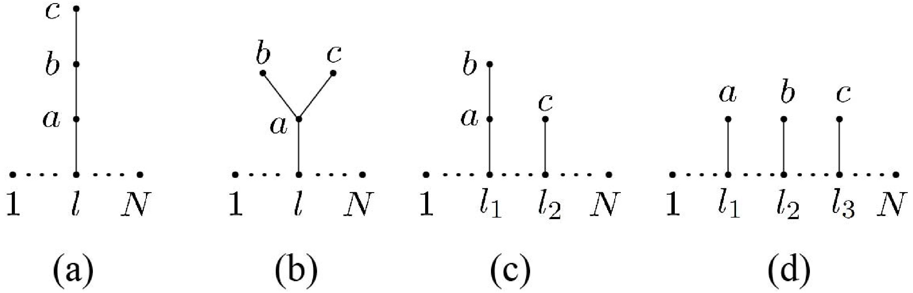

Figure 1

Figure 1.  All possible topologies of spanning forests for the three-graviton example; a, b, and c refer to different gravitons.

DownLoad: Full-Size Img PowerPoint

In the following, we analyze the contribution of each term in Eq. (6).

First, consider the term $\psi_1\psi_{12}\psi_{23}$ on the right hand side of Eq. (6). This term is characterized as shown in Fig. 1 (a) (with $a = 1$, $b = 2$, $c = 3$). Given that

where we have applied the eikonal identity given by Eq. (1) and $s_{ln_1} = [ln_1]\langle n_1l \rangle$, we can express the Parke-Taylor factor accompanied by $\psi_1\psi_{12}\psi_{23}$ as

where the factors $\langle r_1,r_1+1\rangle$ and $\langle t_1,t_1+1\rangle$ in the denominator of the Parke-Taylor factor have been replaced by $\langle r_1,n_1\rangle\langle n_1,r_1+1 \rangle$ and $\langle t_1,n_1\rangle\langle n_1,t_1+1 \rangle$, respectively; $n_1$ in the second Parke-Taylor factor is denoted by $\widetilde n_1$. Hence, graviton $n_1$ splits into gluons $n_1$ and $\widetilde n_1$ with the same momentum and helicity. These gluons are respectively inserted between 1, l and l, N. We can further express $\psi_{12}$ and $\psi_{23}$ as

When Eq. (9) is substituted into Eq. (8), we obtain that graviton $n_2$ splits into gluons $n_2$ and $\widetilde n_2$, which are respectively inserted into the left side of $n_1$ and right side of $\widetilde n_1$. Similarly, Eq. (10) finally inserts gluons $n_3$ and $\widetilde n_3$ corresponding to graviton $n_3$ into the left side of $n_2$ and right side of $\widetilde n_2$. The term $\dfrac{\langle ij\rangle^{4}}{\langle12\rangle\langle23\rangle\cdots\langle N1\rangle}\psi_1\psi_{12}\psi_{23}$ is expressed as

where we have introduced $\text{PT}\left(a_1,...,a_m\right)$ to denote the PT factor $\dfrac{\langle ij\rangle^{4}}{\langle a_1a_2\rangle\langle a_2a_3\rangle\cdots\langle a_ma_1\rangle}$ in short. Permutations ${\boldsymbol{\rho}}^{(l)}$ for a given $l\in\mathrm{G}$ are expressed as

where $A\sqcup\mathchoice{\mkern-7mu}{\mkern-7mu}{\mkern-3.2mu}{\mkern-3.8mu}\sqcup B$ denotes all possible permutations of two ordered sets A and B resulting from merging A and B so that the relative ordering of elements in both A and B is preserved. These permutations can be characterized by the graph shown in Fig. 2 (a).

Figure 2

Figure 2.  (a). Permutations with relative orderings $1,\cdots,$$n_3,\cdots,n_2,\cdots,n_1,\cdots,l,\cdots,\widetilde n_1,\cdots,\widetilde n_2,\cdots,\widetilde n_3,\cdots,N$. (b) Permutations with relative orderings $1,\cdots,n_2,\cdots,n_3,\cdots,n_1,\cdots,$$l,\cdots, \widetilde n_1,\cdots,\widetilde n_3,\cdots,\widetilde n_2,\cdots,N$.

DownLoad: Full-Size Img PowerPoint

The term including $\psi_1\psi_{12}\psi_{13}$ is associated with the graph shown in Fig. 1 (b) (with $a = 1$, $b = 2$, $c = 3$). When factors $\psi_1$ and $\psi_{12}$ are expressed using Eqs. (7) and (9), and $\psi_{13}$ is expressed as

we can split gravitons $n_1$, $n_2$, and $n_3$ into three pairs of gluons, namely $\{n_1,\widetilde n_1\}$, $\{n_2,\widetilde n_2\}$, and $\{n_3,\widetilde n_3\}$, respectively. Gluons $n_1$ and $\widetilde n_1$ coming from graviton $n_1$ are inserted into the left and right sides of l, while $n_2$ and $\widetilde n_2$ (as well as$n_3$ and $\widetilde n_3$) are further inserted into the left side of $n_1$ and right side of $\widetilde n_1$. Thus, this term becomes

where ${\boldsymbol{\rho}}^{(l)}$ for a given l is expressed as

which are characterized in Figs. 2 (a) and (b).

Next, we calculate the term including $\psi_1\psi_{3}\psi_{12}$ (see Fig. 1 (c) for $a = 1$, $b = 2$, and $c = 3$). Applying the same procedure employed in the previous examples, $\psi_1$ and $\psi_{12}$ are expressed in Eqs. (7) and (9), while $\psi_3$ is obtained by replacing $n_1$by $n_3$ in Eq. (7). Again, these factors are used to insert gluon pairs into the Parke-Taylor factor. The result is

where${\boldsymbol{\rho}}^{(l_1,l_2)}$ for given $(l_1,l_2)$ satisfies

In Eq. (12), ${\boldsymbol{\rho}}^{(l_1)}$denotes the permutations established by inserting the collinear gluons corresponding to $n_1$ and $n_2$ into the original gluon set, while ${\boldsymbol{\rho}}^{(l_1)}_{L}$ and ${\boldsymbol{\rho}}^{(l_1)}_{R}$ are the sectors separated by gluon $l_2$in permutation ${\boldsymbol{\rho}}^{(l_1)}$. Possible relative positions of $l_2$ in ${\boldsymbol{\rho}}^{(l_1)}$ are shown in Figs. 3 (a)−(g). Given that the choices of $l_1$ and $l_2$ are independent of each other and we finally summed over all possible choices of $l_1$ and $l_2$, the roles of $l_1$ and $l_2$ in Eq. (12) can be exchanged as follows:

Figure 3

Figure 3.  Possible relative positions of $l_2$ in permutations ${\boldsymbol{\rho}}^{(l_1)}$ in Eq. (12).

DownLoad: Full-Size Img PowerPoint

When all possible spanning forests for the amplitude with three gravitons are considered, the full MHV amplitude with three gravitons can be expressed by the following formula:

In the above expression, we sum over all possible spanning forests where the original gluon set G plays the role of the root set. For a given spanning forest with i ($i\leq 3$) trees, ${\cal{T}}_1,{\cal{T}}_2,\cdots,{\cal{T}}_i$, planted at gluons $l_1,l_2,\cdots,l_i\in \mathrm{G}$ ($l_j$ and $l_k$ with distinct labels may be identical), each $K({\cal{T}}_j)$ ($j = 1,2,\cdots,i$) is expressed as

where $ab\in E({\cal{T}}_j)$ is an edge of tree ${\cal{T}}_j$ with vertices a and b. More explicitly, there are four possible topologies for the three-graviton amplitude, as shown in Figs. 1 (a), (b), (c), and (d), which respectively provide the factors

where a, b, and c represent distinct gravitons. Two graphs that differ only by exchanging the branches attached to the same vertex are considered the same graph, as exemplified in Fig. 1(b). The permutations associated with the topologies shown in Figs. 1(a) and (b) can be recursively defined using Eqs. (11) and (12) by replacing subscripts 1, 2, and 3 of gravitons in Eq. (12) with a, b, and c, respectively. The permutations shown in Fig. 1 (c) satisfy

The permutations associated with the topologies in Fig. 1 (d) are expressed as

We have presented examples with three gravitons. Next, we address the general formula.

IV. GENERAL FORMULA

• I. INTRODUCTION
• II. BACKGROUND
•      A Spinor-helicity formalism in four dimensions
•      B SBDW and spanning forest formulae
• III. AMPLITUDES WITH THREE GRAVITONS
• IV. GENERAL FORMULA
• V. CONCLUSIONS

Inspired by the example in the previous section, we propose the following general formula, where gravitons split into pairs of collinear gluons:

Here, we sum over all possible spanning forests in which trees are planted at gluons $l_1,...,l_i\in\mathrm{G}$. This summation is in turn expressed by two summations:

● (i) Summation over all possible choices of roots $l_1,l_2,\cdots,l_i$ ($i = 1,2,\cdots,M$).

● (ii) For a given choice of roots $l_1,l_2, \cdots$, $l_i$, summation over all possible configurations of forests, which consist of nontrivial trees ${\cal{T}}_1, {\cal{T}}_2,\cdots,$${\cal{T}}_i$ planted at gluons $l_1,l_2, \cdots,$$l_i$.

For a fixed forest, each tree ${\cal{T}}_k$is associated with a factor $K({\cal{T}}_k)$, where each edge between two vertices a and b is assigned by a factor $s_{ab}$. Permutations ${\boldsymbol{\rho}}^{(l_1,l_2,\cdots,l_k)}$ in the PT factors can be defined recursively as

where ${\boldsymbol{\rho}}_L^{(l_1,l_2,\cdots,l_{k-1})}$ and ${\boldsymbol{\rho}}_R^{(l_1,l_2,\cdots,l_{k-1})}$ denote two ordered sets separated by gluon $l_k$ in permutation ${\boldsymbol{\rho}}^{(l_1,l_2,\cdots,l_{k-1})}$; ${\boldsymbol{\sigma}}^{{\cal{T}}_k}$ ($\widetilde{{\boldsymbol{\sigma}}}^{{\cal{T}}_k}$) stands for the permutations established by tree graph ${\cal{T}}_k$ whose nodes are $\{n_i\}$ ($\{\widetilde n_i\}$), while $(\widetilde{{\boldsymbol{\sigma}}}^{{\cal{T}}_k})^T$ denotes the reverse of $\widetilde{{\boldsymbol{\sigma}}}^{{\cal{T}}_k}$.

Next, we outline the proof of the general formula expressed by Eq. (15):

● (i) Step-1. Expand the MHV amplitude according to Eqs. (2) and (5) in terms of spanning forests. In general, each forest F consists of i tree structures, ${\cal{T}}_1, {\cal{T}}_2,\cdots,$${\cal{T}}_i$, planted at gluons $l_1,l_2,\cdots,l_i\in \mathrm{G}$.

● (ii) Step-2. For a given forest $F = \{{\cal{T}}_1,{\cal{T}}_2,\cdots,$${\cal{T}}_i\}$ and tree ${\cal{T}}_1$, there are two types of edges: (a) the edge between a graviton a and the root (a gluon $l_1\in \mathrm{G}$) and (b) the edge between two gravitons b and c. In the former case, the edge is associated with a factor $\psi_{a}$, which is expressed using Eq. (7), while an edge of the latter form is accompanied by a factor $\psi_{bc}$, which can be rewritten as Eq. (9). After this manipulation, factor $\psi_{a}$ splits graviton $n_a$ into collinear gluons $n_a$ and $\widetilde n_a$ and then inserts them into the left and right sides of $l_1$, respectively. A factor $\psi_{bc}$ splits graviton $n_c$ into collinear gluons $n_c$ and $\widetilde n_c$, which are inserted into the left side of $n_b$ and right side of $\widetilde n_b$ ($n_b$, which is closer to the root than $n_c$, has already been treated before). The factor assigned to each edge $bc$ is $s_{bc}$, and the product of all these factors yields $K({\cal{T}}_1)$. The permutations established by this step are expressed as

● (iii) Step-3. Insert the collinear gluons corresponding to the gravitons on trees ${\cal{T}}_2, {\cal{T}}_3,\cdots,$${\cal{T}}_i$ in turn by repeating Step-2. We finally obtain the general formula, Eq. (15), with permutations defined by Eq. (16).

V. CONCLUSIONS

• I. INTRODUCTION
• II. BACKGROUND
•      A Spinor-helicity formalism in four dimensions
•      B SBDW and spanning forest formulae
• III. AMPLITUDES WITH THREE GRAVITONS
• IV. GENERAL FORMULA
• V. CONCLUSIONS

In this note, we present a formula (Eq. (15)) for single-trace EYM amplitudes in MHV configuration (with two negative-helicity gluons). Each graviton in this formula splits into a pair of collinear gluons. Thus, an N-gluon and M-graviton amplitude is expressed as a combination of $N+2M$ gluon amplitudes with M pairs of collinear gluons. When the adjustment described in Section II is considered, Eq. (15) is easily extended to MHV amplitudes with one negative-helicity gluon and one negative-helicity graviton by (i) replacing i and j in the numerator of the PT factor with the negative-helicity graviton and negative-helicity gluon, (ii) using the positive-helicity graviton set instead of the full graviton set on the RHS of Eq. (15), and (iii) adding an extra $(-1)$ in the expression. It would be worthwhile to extend the collinear expression presented in this paper to double-trace amplitudes and amplitudes with other helicity configurations in future studies.

1In this work, we use $$\begin{document}$ \sim $\end{document}$$ to neglect the coupling constant and an overall normalization factor.

References