One-loop analytical expressions for gg/γγ → ϕiϕj in Higgs extensions of the standard model and their applications

Khiem Hong Phan; Dzung Tri Tran; Thanh Huy Nguyen

doi:10.1088/1674-1137/ada3cd

Chinese Physics C> Recent > Article

One-loop analytical expressions for gg/γγ → ϕ_iϕ_j in Higgs extensions of the standard model and their applications

a.
Institute of Fundamental and Applied Sciences, Duy Tan University, Ho Chi Minh City 70000, Vietnam
b.
Faculty of Natural Sciences, Duy Tan University, Da Nang City 50000, Vietnam
c.
VNUHCM-University of Science, 227 Nguyen Van Cu, District 5, Ho Chi Minh City 70000, Vietnam

Abstract
HTML
Reference
Related

PDF

Abstract：
General one-loop formulas for loop-induced processes $gg/\gamma \gamma \rightarrow \phi_i\phi_j$ with $\phi_i\phi_j = hh,~hH,~HH$ are presented in this paper. The analytic expressions evaluated in this study are valid for a class of Higgs Extensions of the Standard Model, e.g., Inert Doublet Higgs, Two Higgs Doublet, Zee-Babu, and Triplet Higgs Models. Analytic expressions for one-loop form factors are expressesd in terms of the basic scalar one-loop two-, three-, and four-point functions following the output format of the packages ${\tt LoopTools}$ and ${\tt Collier}$ . Hence, physical results can be evaluated numerically using one of these packages. The analytic results are tested using several checks such as the ultraviolet finiteness and infrared finiteness of the one-loop amplitudes. Furthermore, the amplitudes obey the ward identity due to massless gauge bosons in the initial states. This identity is also verified numerically. Regarding applications, we present the phenomenological results for the investigated processes in the Zee-Babu model as a typical example. In particular, production cross-sections for the processes $\gamma \gamma\rightarrow hh$ are scanned over the parameter space of the Zee-Babu Model.
- Higgs phenomenology ,
- one-loop corrections ,
- analytic methods for quantum field theory ,
- dimensional regularization

I. INTRODUCTION

I. INTRODUCTION
II. ONE-LOOP CONTRIBUTIONS FOR PROCESSES $gg/\gamma\gamma \rightarrow \phi_i\phi_j$ IN THE HESMs
Ⅲ. APPLICATIONS
     A Numerical tests
     B Standard model
     C Zee-Babu model
IV. CONCLUSIONS
APPENDIX A: TENSOR REDUCTION FOR ONE-LOOP INTEGRALS
APPENDIX B: ANALYTIC RESULTS FOR ONE-LOOP FORM FACTORS
APPENDIX C: LAGRANGIAN FOR ZEE-BABU MODELS

Discovering the structure of scalar potential and consequently answering for the nature of the electroweak symmetry breaking (EWSB) are the most important purposes at future colliders, e.g. the High-Luminosity Large Hadron Collider (HL-LHC) [1, 2], future lepton colliders (LC) [3, 4]. For the purposes, probing for multi-scalar boson productions are great of interest at the future colliders. Because the accuracy production cross-sections provide us not only a crucial information for extracting triple Higgs and quadruple Higgs self-couplings but also direct searches for new scalar particles. In the former case, indirect searches for new physics contributions can be performed through the corrected measurements for Higgs self-couplings. Recently, Standard Model-like (SM-like) Higgs boson pair productions have been probed at the LHC, e.g. via the events of two bottom quarks associated with two photons, four bottom quarks events, etc, as shown in [5−16]. The future lepton colliders are also proposed for complementary to the physics at the LHC, for examples, the LC can significantly improve accuracy the LHC measurements on many observables [17]. More important point, photon-photon collision is considered as an option of the LC [3, 4] which the scalar Higgs pair productions ( $\phi_i\phi_j$ ) can be measured through scattering processes $\ell \bar{\ell} \rightarrow \ell \bar{\ell} \gamma^*\gamma^* \rightarrow \ell \bar{\ell} \phi_i\phi_j$ for $\ell \equiv e, \mu$ . Together with the LHC, the LC also open a good opportunity for discovering many of physics beyond the SM (BSM) via multi-scalar Higgs productions.

In order to match the higher-precision data at the future colliders, theoretical evaluations for one-loop contributing to the di-Higgs boson productions are mandatory. One-loop contributing to the processes at the LHC in the frameworks of the SM, of the Higgs Extensions of the SM (HESM) and other BSMs have performed in many papers, e.g. refering typical works as in Refs. [18−80]. In the high-energy photon-photon collisions, one-loop corrections to the di-Higgs boson productions within the SM and many of BSMs have computed in Refs. [81−95]. At the future linear lepton colliders, including future multi-TeV muon colliders, the equivalent calculations for the Higgs pair productions have considered in Refs. [96−99]. Additionally, one-loop corrections to the scattering processes $\gamma\gamma \rightarrow A^0A^0$ ( $A^0$ is CP-odd Higgs) in Two Higgs Doublet Model have shown in Ref. [100]. The partonic processes $gg/\gamma \gamma \rightarrow \phi_i\phi_j$ play an important role at future colliders. For examples, we can construct the processes $pp\rightarrow \phi_i\phi_j$ at the LHC by convoluting the parton distribution functions for the initial gluons. Another case, one can generate the total cross-sections of the scattering processes $\ell \bar{\ell} \rightarrow \ell \bar{\ell} \gamma^*\gamma^* \rightarrow \ell \bar{\ell} \phi_i\phi_j$ for $\ell \equiv e, \mu$ by the convolution of the mentioned partonic channels with the photon energy spectrum in lepton beams. Subsequently, we can obtain the corresponding cross-sections for scalar boson pair productions at future colliders including multi-TeV muon collider. In the scope of this paper, we present a general one-loop formulas for loop-induced partonic processes $gg/\gamma \gamma \rightarrow \phi_i\phi_j$ with $\phi_i\phi_j = hh,\; hH,\; HH$ which are valid for a class of Higgs Extensions of the Standard Models, e.g. Inert Doublet Higgs Models, Two Higgs Doublet Models, Zee-Babu models as well as Triplet Higgs Models, etc.

In this computation, analytic expressions for one-loop form factors are written in terms of the basic scalar one-loop two-, three- and four-point functions with following the output format of the packages ${\tt LoopTools}$ [102] as well as ${\tt Collier}$ [103]. Numerical investigation can be hence generated by using one of the mentioned packages. Analytic results are confirmed by several checks such as such as the ultraviolet finiteness, infrared finiteness of the one-loop amplitudes. Furthermore, the amplitudes also obey the ward identity due to massless gauge bosons in the initial states. This identity is also verified numerically in the work. In the applications, the phenomenological results for the calculated processes in the Zee-Babu Model are examined as a typical example in this article. Especially, production cross-section for the scattering $\gamma \gamma\rightarrow hh$ are scanned over the parameter space of the model under consideration.

The paper is presented with the structure as follows. Detailed evaluations for one-loop corrections to with CP-even Higgses $\phi_{i,j}\equiv h,\; H_j$ in the HESMs are shown in section 2. We then discuss on the numerical checks for the calculation and show for the applications of this work in the section 3. Conclusion and outlook are devoted in section 4. Analytic expressions for one-loop form factors given in the appendix B. Deriving the additional couplings in the Zee-Babu models are presented in the appendix C.

II. ONE-LOOP CONTRIBUTIONS FOR PROCESSES $gg/\gamma\gamma \rightarrow \phi_i\phi_j$ IN THE HESMs

I. INTRODUCTION
II. ONE-LOOP CONTRIBUTIONS FOR PROCESSES $gg/\gamma\gamma \rightarrow \phi_i\phi_j$ IN THE HESMs
Ⅲ. APPLICATIONS
     A Numerical tests
     B Standard model
     C Zee-Babu model
IV. CONCLUSIONS
APPENDIX A: TENSOR REDUCTION FOR ONE-LOOP INTEGRALS
APPENDIX B: ANALYTIC RESULTS FOR ONE-LOOP FORM FACTORS
APPENDIX C: LAGRANGIAN FOR ZEE-BABU MODELS

In this section, detailed evaluations for one-loop contributions for the scattering processes $gg/\gamma\gamma \rightarrow \phi_i\phi_j$ in the HESMs are shown in this section. We first arrive at the concrete evaluations for the processes $\gamma\gamma \rightarrow \phi_i\phi_j$ . We then extend these results to the processes $gg \rightarrow \phi_i\phi_j$ .

Additional scalar bosons in the mentioned HESMs are included as CP-even Higgses $\phi_i$ , CP-odd Higgses $A_j^{0}$ and singly (doubly) charged Higgses $S\equiv S_k^Q$ with charged quantum number Q, for $i,j, k = 1,2,\cdots$ . In this work, $S_k^Q$ can be singly charged Higgs $H^{\pm}$ and doubly charged Higgs $K^{\pm\pm}$ , appropriately. Beyond the SM, the extra couplings relating to the mentioned scalar particles in the HESMs are parameterized as general form $g_{\text{vertex}}$ . Explicitly formulas for $g_{\text{vertex}}$ for each model under investigation are presented in concrete, seen Zee-Babu Model in the application of this work and our previous work [104] for examples.

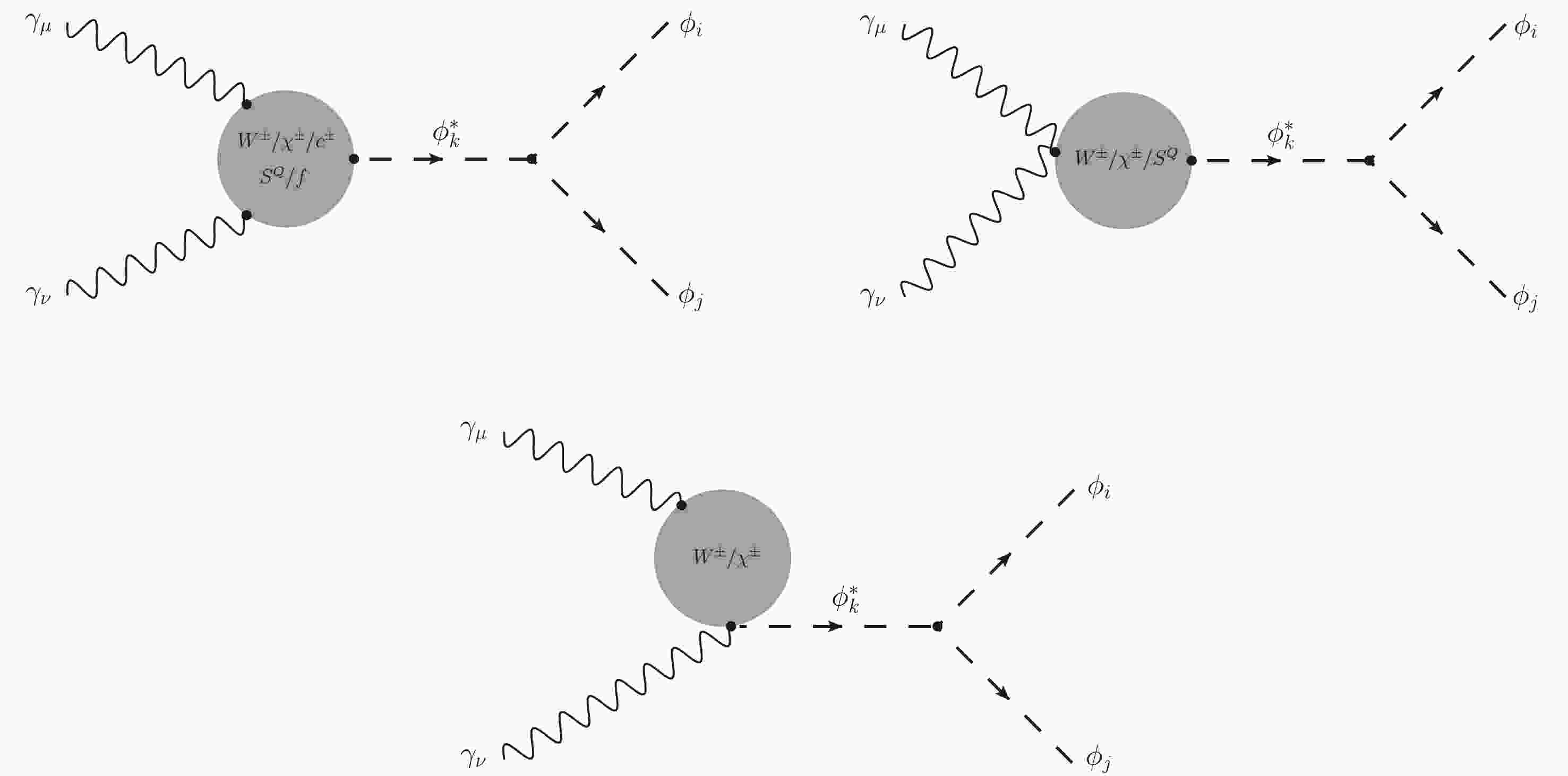
By employing the on-shell renormalization scheme developed in [113−115] for the fermion sector and gauge sector as well as the improved on-shell renormalization scheme for the scalar sector following the method in [116], one loop-induced Feynman diagrams for the production processes $\gamma \gamma \rightarrow \phi_i \phi_j$ with CP-even Higgses $\phi_{i,j} \equiv h, H$ in the HESMs are plotted in the following paragraphs. The calculations are handled in the't Hooft-Feynman (HF) gauge which one loop-induced Feynman diagrams can be categorized into several groups as explained in below. We mention the first classification Feynman diagrams as shown in Fig. 1. In this group, we list all one-loop diagrams with $\phi_k^*$ -poles for $\phi_k^* = h^*,\; H^*$ . These kinds of diagrams appear in this group are included all one-loop diagrams contributions for off-shell CP-even Higges decay like $\phi_k^* \rightarrow \gamma\gamma$ with fermions (noted as $G_1$ ), W-boson, charged Goldstone $\chi^{\pm}$ , Ghosht particles $c^\pm$ (as $G_2$ ) and charged Higges $S^{Q}$ (as $G_3$ ) internal lines in connecting with the vertices $\phi_k^*\phi_i\phi_j$ .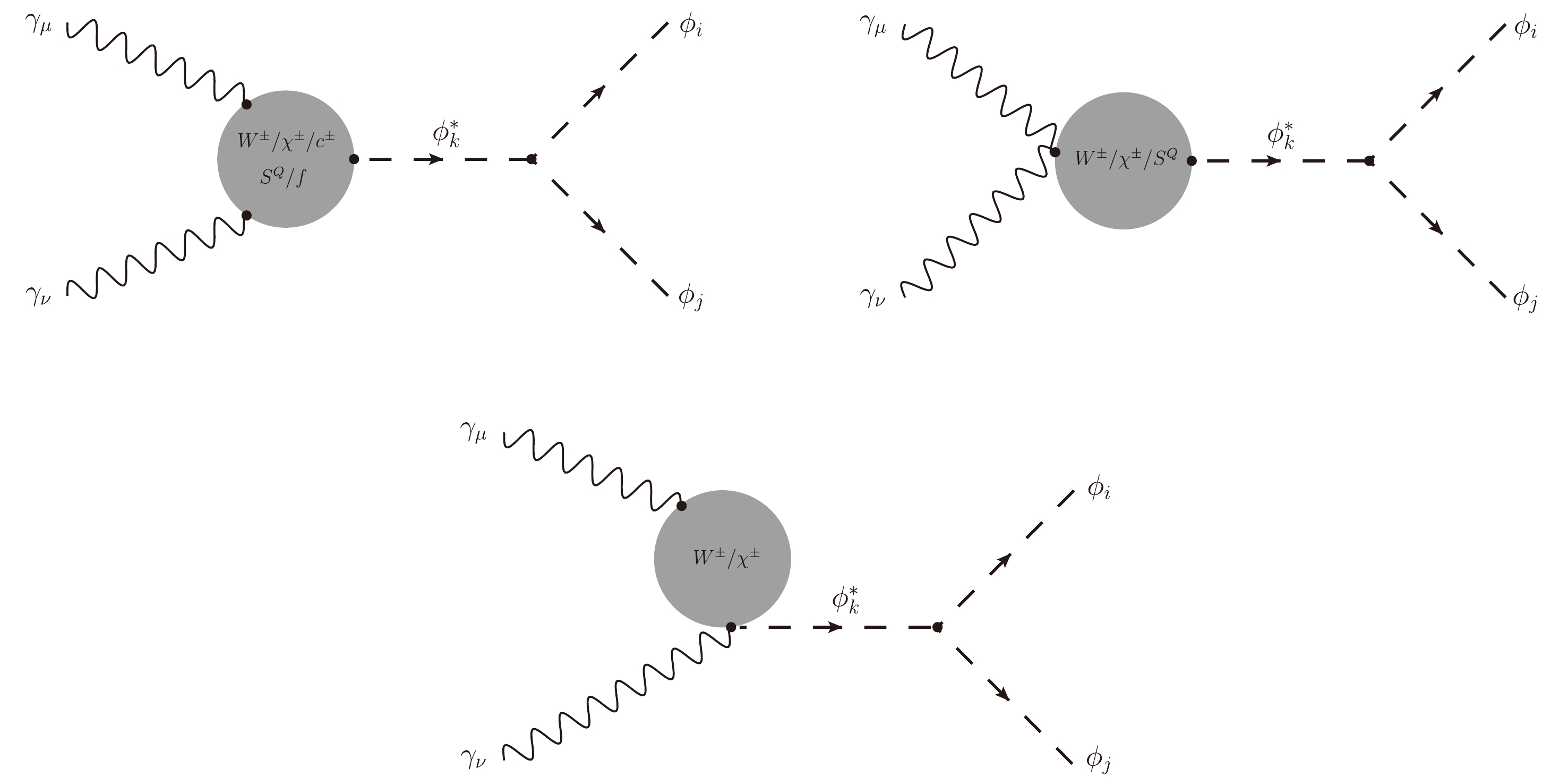

Figure 1

Figure 1. All one-loop diagrams with fermions, W bosons (with charged Goldstone

$\chi^{\pm}$ , Ghosht particles

$c^\pm$ ) and charged Higges exchanging in the loop of

$\phi_k^*$ -poles, for

$\phi_k^*=h^*, H^*$ . These kinds of diagrams appear in this group are included one-loop contributions for off-shell CP-even Higges decay like

$\phi_k^* \rightarrow \gamma\gamma$ in connecting with the vertices

$\phi_k^*\phi_i\phi_j$ .

DownLoad: Full-Size Img PowerPoint

The second classification of one-loop Feynman diagrams is involed to the one-loop box diagrams. The first type of box diagrams contributing to the computed processes is plotted as in Fig. 2. In these topologies, all fermions internal lines are taken into consideration (noted as group $G_4$ ).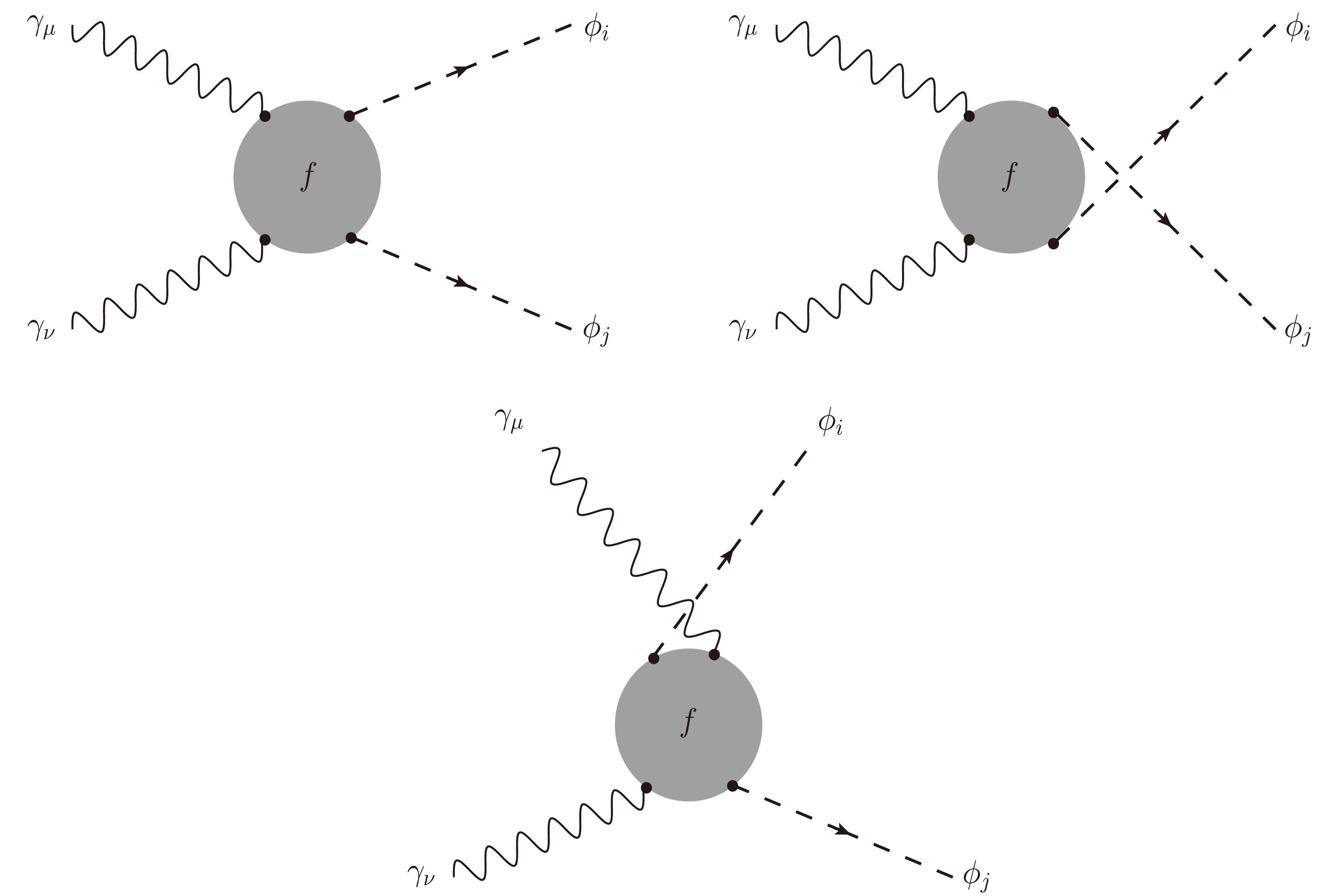

Figure 2

Figure 2. One-loop four external legs with fermion internal lines contributing to the computed processes (noted as group

$G_4$ ).

DownLoad: Full-Size Img PowerPoint

Additionally, the second type of one-loop four-point Feynman diagrams with vector W-bosons, the charged Goldstone bosons $\chi^{\pm}$ , Ghosht particles $c^\pm$ internal lines are concerned in the calculated processes. These diagrams are grouped into $G_5$ as shown in Figs. 3, 4.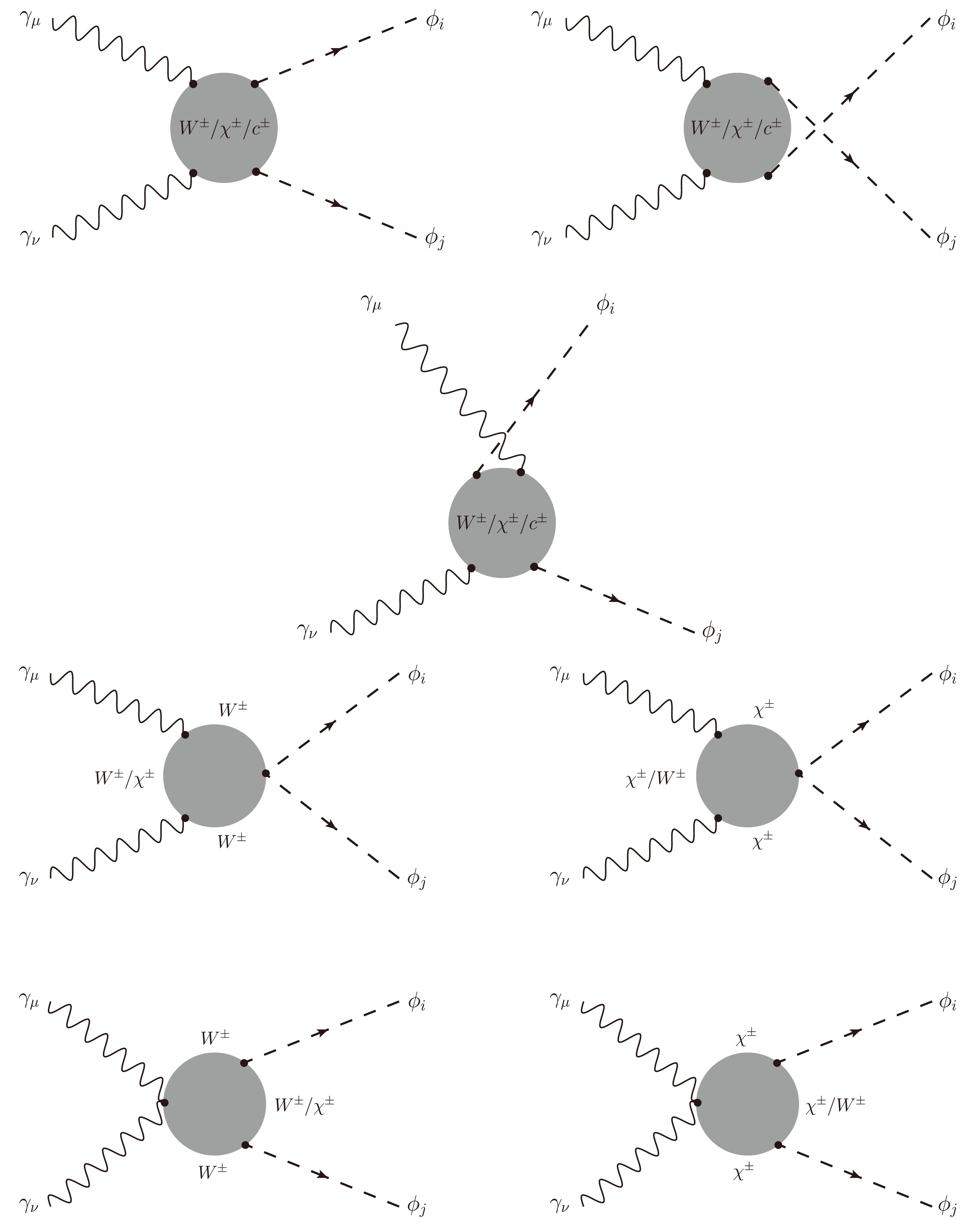

Figure 3

Figure 3. All one-loop box diagrams contributing to the processes with W-boson exchanging in the loop (putted into

$G_5$ ).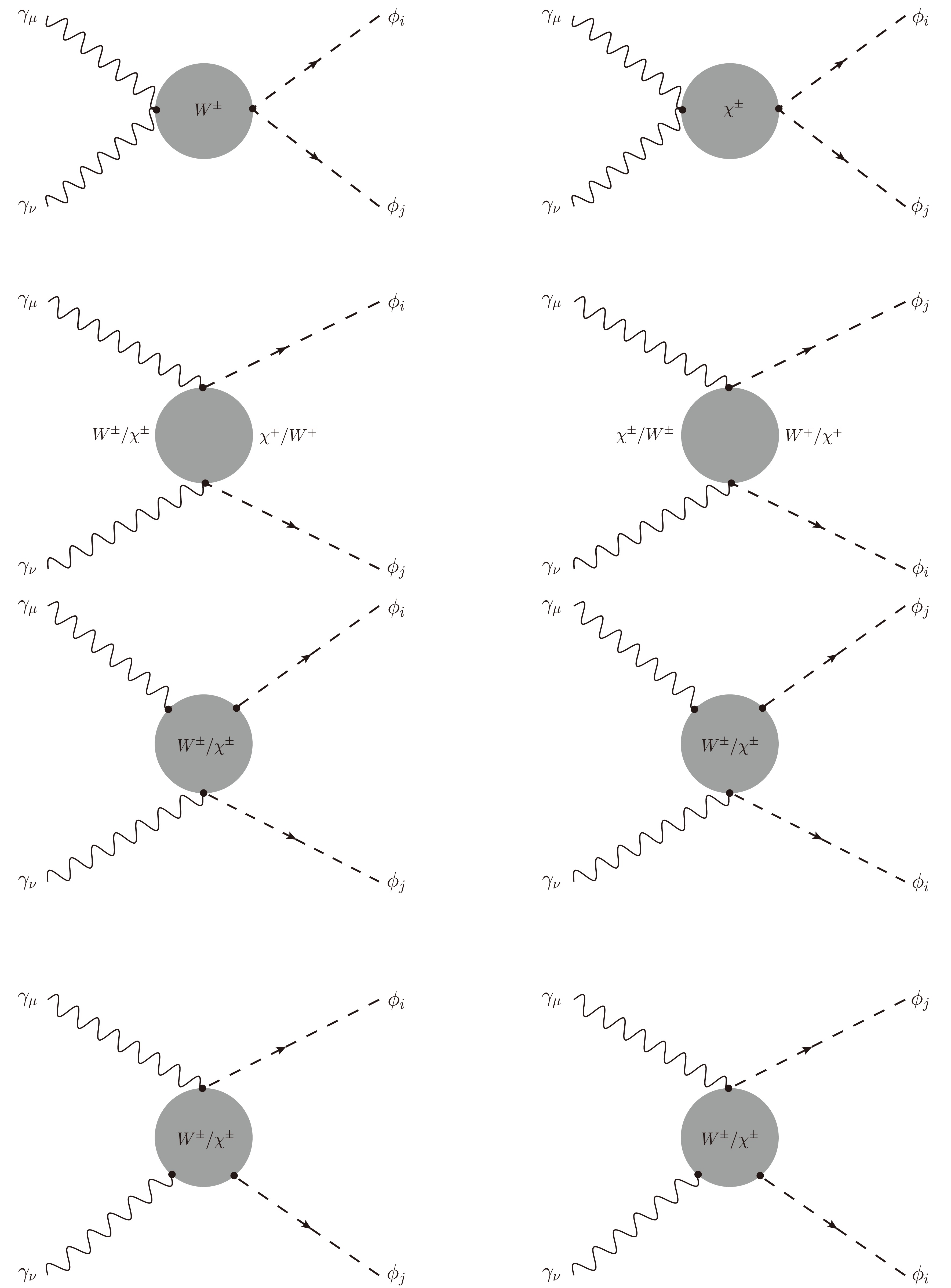

DownLoad: Full-Size Img PowerPoint

Figure 4

Figure 4. All one-loop box diagrams contributing to the processes with W-boson exchanging in the loop (putted into

$G_5$ ).

DownLoad: Full-Size Img PowerPoint

In the scope of the HESMs concerned in this work, we have also another type pf one-loop box diagrams with both W-boson and singly charged Higgs $S^{Q} \equiv H^{\pm}$ propagating in the loop, seen Figs. 5, 6. We put these diagrams into group $G_6$ .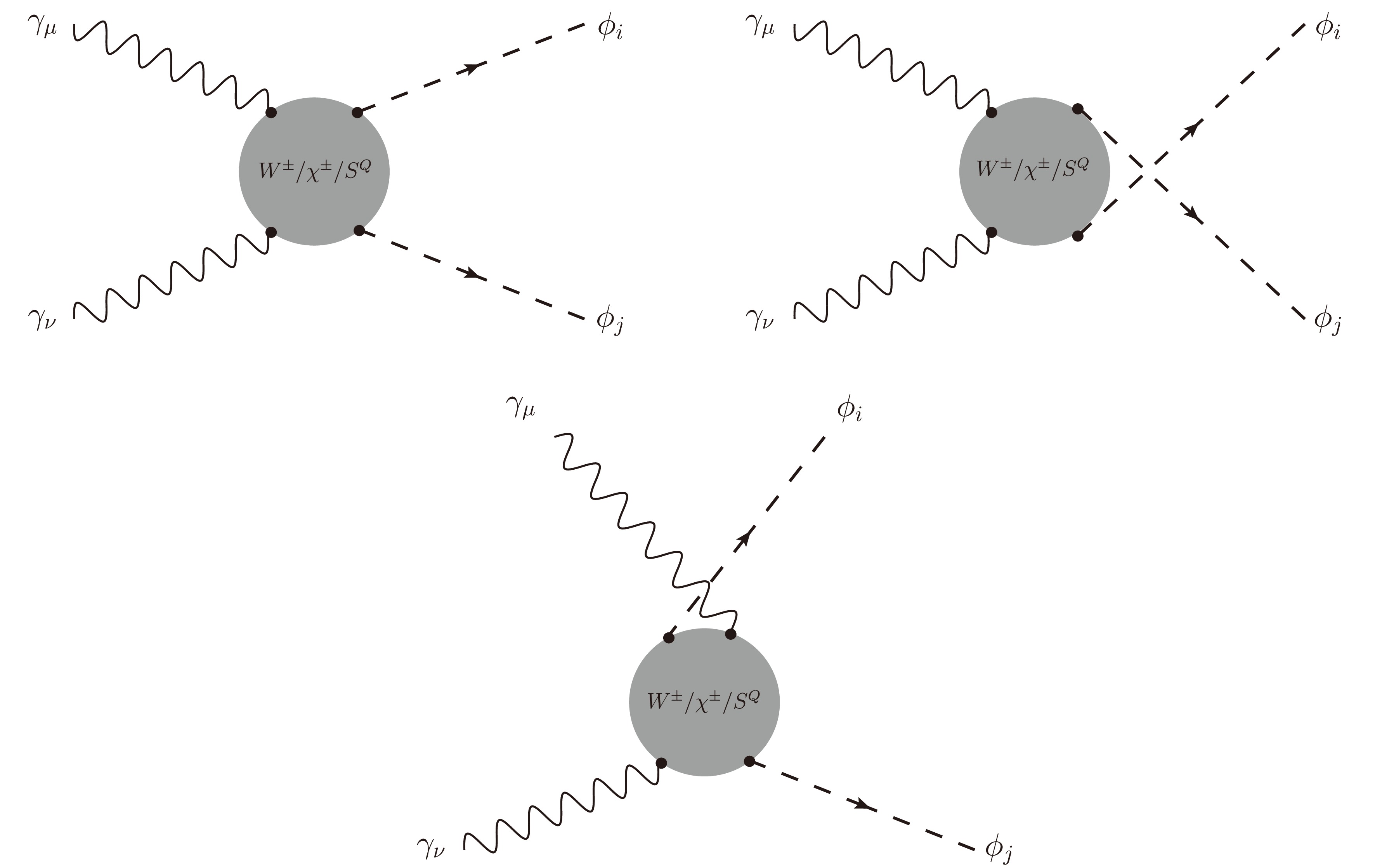

Figure 5

Figure 5. One-loop box diagrams with both W-boson and charged Higgs propagating in the loop (putted into

$G_6$ ).

DownLoad: Full-Size Img PowerPoint

Figure 6

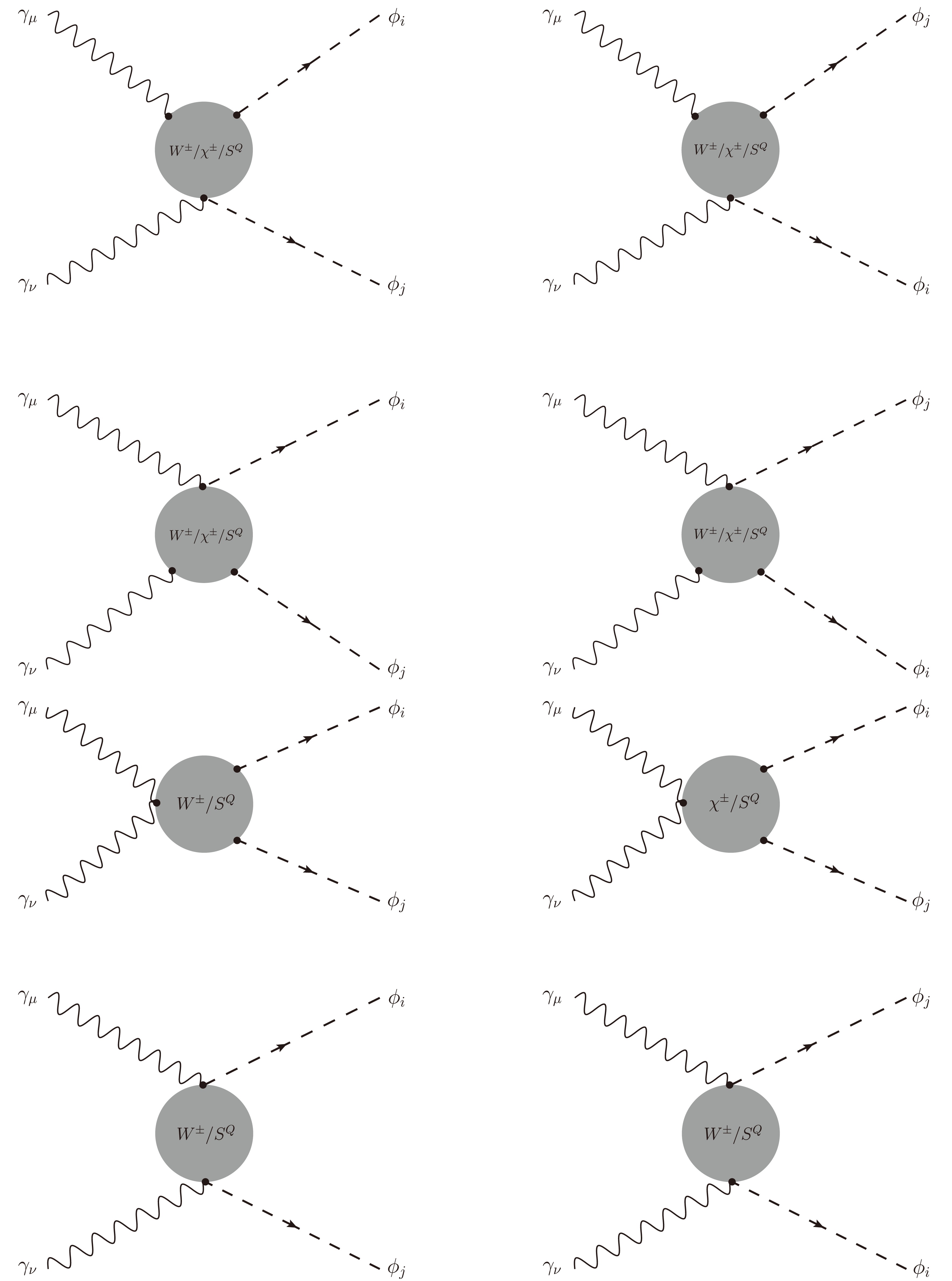
Figure 6. Further one-loop box diagrams with both W-boson and charged Higgs propagating in the loop (putted into

$G_6$ ).

DownLoad: Full-Size Img PowerPoint

Finally, we consider the last type of one-loop box diagrams with charged Higgses $S^{Q} \equiv H^{\pm},\; K^{\pm\pm}$ in the loop, as shown in Fig. 7. We then added these diagrams in to $G_7$ . Both singly charged and doubly charged Higges are considered being internal line particles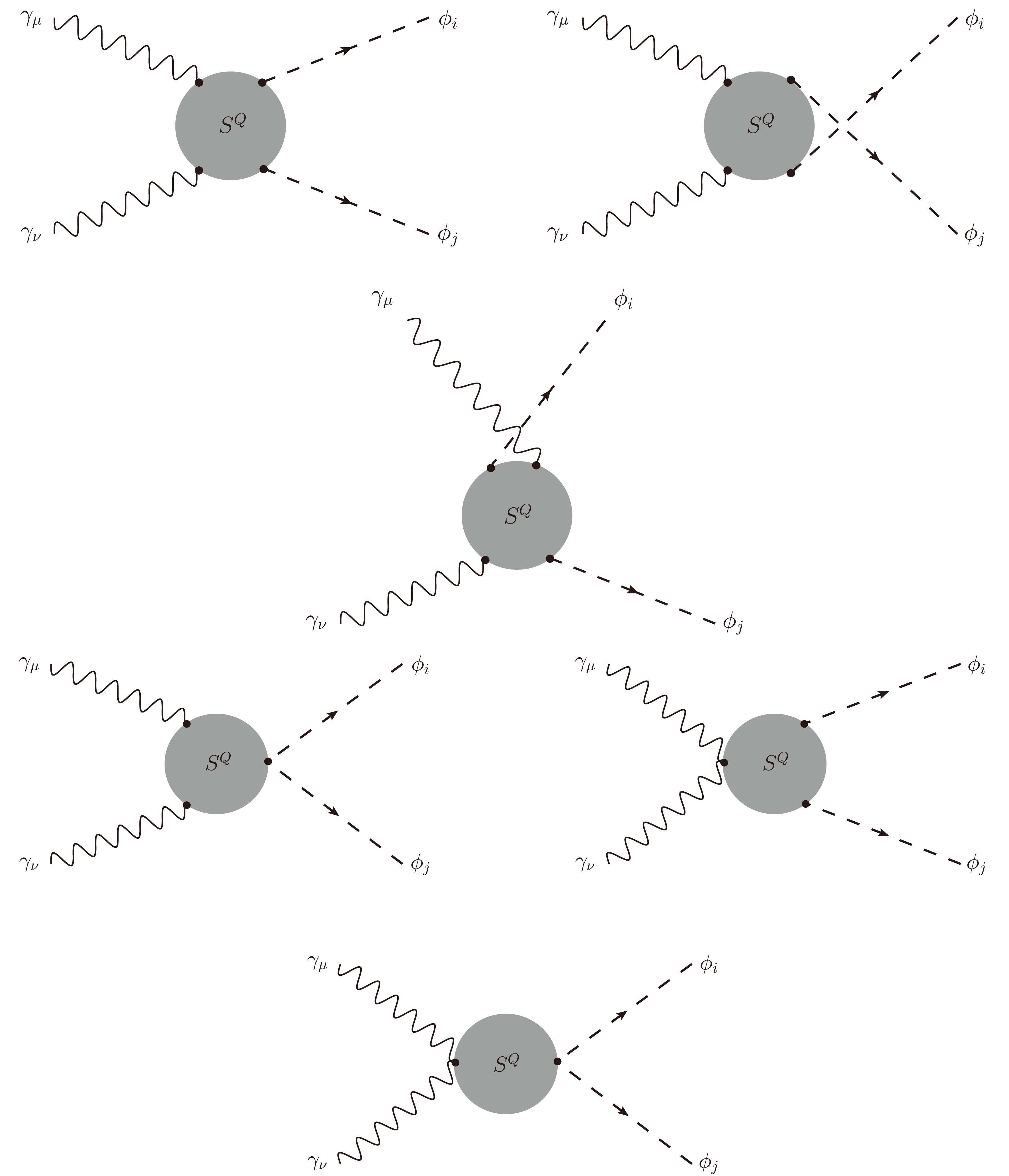 in this case.

Figure 7

Figure 7. All one-loop box diagrams with charged Higgs in the loop (considered as

$G_7$ ).

DownLoad: Full-Size Img PowerPoint

We turn out our attention to discuss on analytic results. In general, one-loop amplitude for scattering processes $\gamma_\mu (q_1) \, \gamma_\nu (q_2) \rightarrow \phi_i (q_3) \, \phi_j (q_4)$ is presented in terms of Lorentz structure as follows:

${\mathcal{A}}_{\gamma \gamma \rightarrow \phi_i \phi_j} = \Big[ F_{00}^{(\gamma\gamma)} \; g^{\mu\nu} + \sum\limits_{i,j = 1; i\leq j}^{3} F_{ij}^{(\gamma\gamma)} \; q_i^{\nu} q_j^{\mu} \Big] \varepsilon_{\mu}(q_1) \varepsilon_{\nu}(q_2).$

(1)

In this formulas, the vector $\varepsilon_{\mu}(q)$ is polarization vector of external photon with the 4-dimension momentum q. The scalar coefficients $F_{ij}^{(\gamma\gamma)}$ for $i,j = 1,2,3$ are called as one-loop form factors. They are written as functions of the following kinematic invariant variables:

$\hat{s} = (q_1+q_2)^2 = q_1^2 + 2 q_1 \cdot q_2 + q_2^2 = 2 q_1 \cdot q_2,$

(2)

$\hat{t} = (q_1 - q_3)^2 = q_1^2 - 2 q_1 \cdot q_3 + q_3^2 = M_{\phi_i}^2 - 2 q_1 \cdot q_3,$

(3)

$\hat{u} = (q_2 - q_3)^2 = q_2^2 - 2 q_2 \cdot q_3 + q_3^2 = M_{\phi_i}^2 - 2 q_2 \cdot q_3.$

(4)

The kinematic invariant masses for external legs are given as $q_1^2 = q_2^2 = 0$ , $q_3^2 = M_{\phi_i}^2$ , $q_4^2 = M_{\phi_j}^2$ . These variables obey the follow identity as $\hat{s} + \hat{t} + \hat{u} = M_{\phi_i}^2 + M_{\phi_j}^2$ . Associated with two massless photons in the initial states, one loop-induced amplitude must satisfy the ward identity. As a result, we derive the following relations among the form factors as:

$F_{00}^{(\gamma\gamma)} = \dfrac{ \hat{t} - M_{\phi_i}^2 }{2} \, F_{13}^{(\gamma\gamma)} - \dfrac{ \hat{s} }{2} \, F_{12}^{(\gamma\gamma)},$

(5)

$F_{00}^{(\gamma\gamma)} = \dfrac{ \hat{u} - M_{\phi_i}^2}{2} \, F_{23}^{(\gamma\gamma)} - \dfrac{ \hat{s} }{2} \, F_{12}^{(\gamma\gamma)},$

(6)

$F_{13}^{(\gamma\gamma)} = \dfrac{ \hat{u} - M_{\phi_i}^2} { \hat{s} } \, F_{33}^{(\gamma\gamma)},$

(7)

$F_{23}^{(\gamma\gamma)} = \dfrac{ \hat{t} - M_{\phi_i}^2} { \hat{s} } \, F_{33}^{(\gamma\gamma)}.$

(8)

Using the mentioned above relations, one-loop amplitude is expressed via two independent one-loop form factors, e.g. taking $F_{12}^{(\gamma\gamma)}$ and $F_{33} ^{(\gamma\gamma)}$ as an example. In detail, the amplitude can be rewritten as follows:

${\cal{A}}_{\gamma \gamma \rightarrow \phi_i \phi_j} = \Big[ {\cal{P}}^{\mu\nu} \cdot F_{12}^{(\gamma\gamma)} + {\mathcal{Q} }^{\mu\nu} \cdot F_{33}^{(\gamma\gamma)} \Big] \, \varepsilon_{\mu}(q_1) \varepsilon_{\nu}(q_2).$

Where two given tensors are defined as

${\cal{P}}^{\mu\nu} = q_2^{\mu} q_1^{\nu} - \dfrac{ \hat{s} }{2} \cdot g^{\mu\nu},$

(9)

${\cal{Q}}^{\mu\nu} = \dfrac{(M_{\phi_i}^2 - \hat{t}) (M_{\phi_i}^2 - \hat{u})}{2 \hat{s} } \cdot g^{\mu\nu} + q_3^{\mu} q_3^{\nu} + \dfrac{( \hat{t} -M_{\phi_i}^2)} { \hat{s} } \cdot q_2^{\mu} q_3^{\nu}.$

(10)

Analytic results for one-loop form factors $F_{12}^{(\gamma\gamma)}$ and $F_{33}^{(\gamma\gamma)}$ for the considered processes in the HESMs are collected in terms of the basic scalar one-loop functions. The form factors $F_{ab}^{(\gamma\gamma)}$ for $ab = \{12, 33\}$ are decomposed into triangle and box parts which are corresponding to the contributions from one-loop triangle and one-loop box diagrams shown in above paragraphs. In detail, the form factor are expressed as follows:

$\begin{aligned}[b] F_{12}^{(\gamma\gamma)} = \;& \sum\limits_{\phi_k^* = h^*, H^*} \dfrac{g_{\phi_k^* \phi_i \phi_j}} {\Big[ s - M_{\phi_k}^2 +i \Gamma_{\phi_k} M_{\phi_k} \Big] } \times \Bigg[ \sum\limits_{f} g_{\phi_k^* ff} \cdot C^{\gamma\gamma}_f \cdot F_{12,f}^{\text{Trig}} + g_{\phi_k^* WW } \cdot F_{12,W}^{\text{Trig}} + \sum\limits_{S = H^{\pm}, K^{\pm\pm}} g_{\phi_k^*SS } \cdot F_{12,S}^{\text{Trig}} \Bigg] \\ & + \sum\limits_{f} g_{\phi_i ff} \cdot g_{\phi_j ff} \cdot C^{\gamma\gamma}_f \cdot F_{12,f}^{\text{Box}} + \Big[ g_{\phi_i W W} \cdot g_{\phi_j WW } \cdot F_{12,W}^{\text{Box, 1}} + g_{\phi_i \phi_j WW } \cdot F_{12,W}^{\text{Box, 2}} + g_{\phi_i \phi_j \chi\chi } \cdot F_{12,W}^{\text{Box, 3}} \Big] \\ & + \sum\limits_{S = H^{\pm}, K^{\pm\pm}} \Big[ g_{\phi_i SS} \cdot g_{\phi_j SS} \cdot F_{12,S}^{\text{Box},1} + g_{\phi_i \phi_j SS} \cdot F_{12,S}^{\text{Box},2} \Big] + g_{\phi_i H^{\pm} W^{\mp}} \cdot g_{\phi_j H^{\pm} W^{\mp}} \cdot F_{12,W, H^\pm}^{\text{Box}},\end{aligned}$

(11)

$F_{33}^{(\gamma\gamma)} = \sum\limits_{f} g_{\phi_i ff} \cdot g_{\phi_j ff} \cdot C^{\gamma\gamma}_f \cdot F_{33,f}^{\text{Box}} + g_{\phi_i W W} \cdot g_{\phi_j W W} \cdot F_{33,W}^{\text{Box}} + \sum\limits_{S^Q = H^{\pm}, K^{\pm\pm}} g_{\phi_i SS} \cdot g_{\phi_j SS} \cdot F_{33,S}^{\text{Box}} + g_{\phi_i H^{\pm} W^{\mp}} \cdot g_{\phi_j H^{\pm} W^{\mp}} \cdot F_{33,W, H^\pm}^{\text{Box}}.$

(12)

In the above equations, $C^{\gamma\gamma}_f = N_C^{f} (eQ_f)^2$ for the decay process $\gamma \gamma \rightarrow \phi_i\phi_j$ . Where $Q_f\; (N_C^f)$ is denoted for charged (color) quantum number of the corresponding fermion f. We note that S is for both singly charged Higgs $H^\pm$ and doubly charged Higgs $K^{\pm\pm}$ in the above formulas. The first contributions to one-loop form factors $F_{12}^{(\gamma\gamma)}$ are calculated from one-loop diagrams appear in off-shell CP-even Higges decay like $\phi_k^* \rightarrow \gamma\gamma$ connecting with the vertices $\phi_k^*\phi_i\phi_j$ (as plotted in Fig. 1). They are decomposed into each term in the bracket, e.g. $F_{12,f}^{\text{Trig}}$ (from fermions f in the loop of $G_1$ in Fig. 1), $F_{12,W}^{\text{Trig}}$ (from W boson in the loop of $G_2$ in Fig. 1), $F_{12,S}^{\text{Trig}}$ (from charged Higges in the loop of $G_3$ in Fig. 1). Secondly, one-loop factors $F_{12,f}^{\text{Box}}$ are computed from the fermions f exchanging in the box diagrams as in Fig. 2. One-loop form factors collected from one-loop W boson propagating in the box diagrams as in Fig. 3, can be divided into the following parts, e.g. $F_{12,W}^{\text{Box, k}}$ for $k = 1,2,3$ which are corresponding to the factors factorized out by general trilinear-couplings of $\phi_i WW, \phi_j WW$ , quadratic-couplings of $\phi_i\phi_j WW$ and $\phi_i\phi_j \chi\chi$ as in Eq. 11. We also express the factors attributing from one-loop charged Higgs in the box diagrams into two sub-factors $F_{12,S}^{\text{Box},k}$ for $k = 1,2$ which are factorized out by general trilinear-couplings of $\phi_i SS,\; \phi_j SS$ , quadratic-couplings of $\phi_i\phi_j WW$ and $\phi_i\phi_j SS$ as in Eq. 11. Lastly, from diagrams with mixing W boson and singly charged Higgs in the loop, we have the factors $F_{12,WH^\pm}^{\text{Box}}$ which can be factorized out in term of the trilinear-couplings $\phi_i H^\pm\; W,\; \phi_jH^\pm\; W$ . Otherwise, the form factors $F_{33}^{(\gamma\gamma)}$ are only contributed from one-loop box diagrams. They can be factorized out in term of general couplings as in Eq. 12. Analytic results for one-loop form factors given in Eqs. 11, 12 are shown explicitly in the appendix B.

Analytic results presented in the above paragraphs can be extended to the channels $gg \rightarrow \phi_i\phi_j$ . There aren't W bosons and charged Higgs propagating in the loop diagrams of the processes $gg\rightarrow \phi_i\phi_j$ . All one-loop Feynman diagrams with f exchanging in the loop are taken into account in this case. In detail, the first diagram $G_1$ in Fig. 1 and all diagrams $G_4$ in Fig. 2 are contributed to the processes $gg\rightarrow \phi_i\phi_j$ . Subsequently, all one-loop form factors $F_{12,W}^{\text{Trig}}$ , $F_{12,S}^{\text{Trig}}$ , $F_{ab,W}^{\text{Box}}$ , $F_{ab,S}^{\text{Box}}$ and $F_{ab,WH^{\pm}}^{\text{Box}}$ for $ab = \{12, 33\}$ are being to zero in this case. Finally, one-loop form factors in the channels $gg\rightarrow \phi_i\phi_j$ are expressed as follows

$\begin{aligned}[b] F_{12}^{(gg)} = \;& \sum\limits_{f} \sum\limits_{\phi_k^* = h^*, H^*} C^{gg}_f \cdot \dfrac{ g_{\phi_k^* \phi_i \phi_j}} {\Big[ s - M_{\phi_k}^2 +i \Gamma_{\phi_k} M_{\phi_k} \Big] } \\& \Bigg[ g_{\phi_k^* ff} \cdot F_{12,f}^{\text{Trig}} + g_{\phi_i ff} \cdot g_{\phi_j ff} \cdot F_{12,f}^{\text{Box}} \Big], \end{aligned}$

(13)

$F_{33}^{(gg)} = \sum\limits_{f} C^{gg}_f \cdot g_{\phi_i ff} \cdot g_{\phi_j ff} \cdot F_{33,f}^{\text{Box}}.$

(14)

Where $C^{gg}_f = \sqrt{2}g_s^2$ with $g_s = \sqrt{4\pi \alpha_s}$ . $\alpha_s$ is strong coupling constant.

Having all the necessary form factors, the cross sections are then evaluated as follows

$\hat{\sigma}_{\rm{HESM}} ^{gg/\gamma\gamma \rightarrow \phi_i \phi_j}(\hat{s}) = \dfrac{1}{n!} \dfrac{1}{16 \pi \hat{s}^2} \int \limits_{t_\text{min}} ^{t_\text{max}} d \hat{t}\; \frac{1}{4} \sum \limits_\text{unpol.} \big| {\cal{A}}_{gg/\gamma \gamma \rightarrow \phi_i \phi_j} \big|^2$

(15)

with $n = 2$ if the final particles are identical such as $gg/\gamma \gamma \rightarrow hh, HH$ , and 1 otherwise like $gg/\gamma \gamma \rightarrow h H$ . The integration limits are

$\begin{aligned}[b] t_{\text{min} (\text{max})} =\; & -\dfrac{\hat{s}}{2} \Bigg\{ 1 - \dfrac{M_{\phi_i}^2 + M_{\phi_j}^2}{s} \pm \Bigg[ 1 - 2 \Bigg( \dfrac{M_{\phi_i}^2 + M_{\phi_j}^2}{s} \Bigg) \\& + \Bigg( \dfrac{M_{\phi_i}^2 - M_{\phi_j}^2}{s} \Bigg)^2 \Bigg]^{1/2} \Bigg\}. \end{aligned}$

(16)

Total amplitude is given

$\begin{aligned}[b] \frac{1}{4} \sum \limits_\text{unpol.} \big| {\cal{A}}_{gg/\gamma \gamma \rightarrow \phi_i \phi_j} \big|^2 = \;&\dfrac{ M_{\phi_i}^4 \; \hat{s}^2 + ( M_{\phi_i}^2 M_{\phi_j}^2 - \hat{t}\; \hat{u} )^2 } {8\; \hat{s}^2} \, \big| F_{33}^{(gg/\gamma\gamma)} \big|^2 \\ & - \dfrac{ M_{\phi_i}^2 \hat{s} } {4} \, {\cal{R}}e \Big[ F_{33}^{(gg/\gamma\gamma)} \cdot \big( F_{12}^{(gg/\gamma\gamma)} \big)^* \Big] + \\& \dfrac{ \hat{s}^2 } {8} \, \big| F_{12}^{(gg/\gamma\gamma)} \big|^2 . \end{aligned}$

Ⅲ. APPLICATIONS

I. INTRODUCTION
II. ONE-LOOP CONTRIBUTIONS FOR PROCESSES $gg/\gamma\gamma \rightarrow \phi_i\phi_j$ IN THE HESMs
Ⅲ. APPLICATIONS
     A Numerical tests
     B Standard model
     C Zee-Babu model
IV. CONCLUSIONS
APPENDIX A: TENSOR REDUCTION FOR ONE-LOOP INTEGRALS
APPENDIX B: ANALYTIC RESULTS FOR ONE-LOOP FORM FACTORS
APPENDIX C: LAGRANGIAN FOR ZEE-BABU MODELS

We are going to present the phenomenological results for this work. We consider two typical applications in this work which are the SM and Zee-Babu Model. We work in the $G_{\mu}$ -scheme and use the input parameters in the SM as same as our previous papers [117, 118]. In the phenomenological results for Zee-Babu model, the parameter space will be taken appropriately in the next subsections. Hereafter, we only discuss the partonic processes $\gamma\gamma \rightarrow \phi_i \phi_j$ as typical example for the numerical tests as well as for the phenomenological analysis.

A Numerical tests

I. INTRODUCTION
II. ONE-LOOP CONTRIBUTIONS FOR PROCESSES $gg/\gamma\gamma \rightarrow \phi_i\phi_j$ IN THE HESMs
Ⅲ. APPLICATIONS
     A Numerical tests
     B Standard model
     C Zee-Babu model
IV. CONCLUSIONS
APPENDIX A: TENSOR REDUCTION FOR ONE-LOOP INTEGRALS
APPENDIX B: ANALYTIC RESULTS FOR ONE-LOOP FORM FACTORS
APPENDIX C: LAGRANGIAN FOR ZEE-BABU MODELS

We first perform numerical tests for the calculations. The form factors must be the ultraviolet finiteness and the infrared finiteness. Furthermore, one-loop amplitude must follow the ward identity due to the initial photons. Numerical checks for the ultraviolet finiteness, infrared finiteness for one-loop form factors are shown in Table 1. For this test, we set the couplings $\lambda_{H\Phi} = +2$ , $\lambda_{K\Phi} = -1$ and the charged scalar masses as follows: $M_{H^\pm} = 500$ GeV, $M_{K^{\pm\pm}} = 1000$ GeV. Additional, one sets $\hat{s} = 1500^2$ GeV, $\hat{t} = -200^2$ GeV². By varying the parameters $C_{UV},\; \lambda^2$ (see appendix A for the definition of these parameters) in a wide range, we find that the results are good stability up to last digits (over 15 digits at the amplitude level).

Table 1

Table 1. Numerical checks for the UV- and IR- finiteness for one-loop form factor

$F_{12}^{(\gamma\gamma)}$ ,

$F_{33}^{(\gamma\gamma)}$ . For this test, we set the couplings

$\lambda_{H\Phi}=+2$ ,

$\lambda_{K\Phi}=-1$ and the charged scalar Higgs masses as follows:

$M_{H^\pm}=500$ GeV,

$M_{K^{\pm\pm}}=1000$ GeV. Additional, one sets

$\hat{s} =1500^2$ GeV²,

$\hat{t} = -200^2$ GeV².

$\big( C_{UV}, \lambda^2 \big)$	$F_{12}^{(\gamma\gamma)}$	$F_{33}^{(\gamma\gamma)}$
$(0,1)$	$-4.432377929637615 \cdot 10^{-10}$	$-1.274104987282513 \cdot 10^{-8}$
	$+ 7.427714924247333 \cdot 10^{-10} \, i$	$+ 2.439535005865118 \cdot 10^{-7} \, i$
$(10^2, 10^4)$	$-4.432377929637721 \cdot 10^{-10}$	$-1.274104987282583 \cdot 10^{-8}$
	$+ 7.427714924247333 \cdot 10^{-10} \, i$	$+ 2.439535005865118 \cdot 10^{-7} \, i$
$(10^4, 10^8)$	$-4.432377929637489 \cdot 10^{-10}$	$-1.274104987282561 \cdot 10^{-8}$
	$+ 7.427714924247333 \cdot 10^{-10} \, i$	$+ 2.439535005865118 \cdot 10^{-7} \, i$

DownLoad: CSV

Show Table

Due to the initial photons taking part in the scattering processes, one-loop amplitude must follow the ward identity. The identity is verified numerically in this work. This can be done as follows. We collect analytic results for one-loop form factors $F_{00}^{(\gamma\gamma)}$ , $F_{12}^{(\gamma\gamma)}$ , $F_{23}^{(\gamma\gamma)}$ and $F_{33}^{(\gamma\gamma)}$ independent way. All the relations in Eqs. 5, 6, 7, 8 are confirmed numerically. The form factors $F_{TT}^{(\gamma\gamma)}$ is given

$F_{TT}^{(\gamma\gamma)} = \dfrac{\hat{u} - M_{\phi_i}^2}{2} \cdot \dfrac{\hat{t} - M_{\phi_i}^2}{\hat{s} } \cdot F_{33}^{(\gamma\gamma)} - \dfrac{\hat{s} }{2} \cdot F_{12}^{(\gamma\gamma)}.$

(17)

One then verifies numerically the equation that $F_{TT}^{(\gamma\gamma)} = F_{00}^{(\gamma\gamma)}$ . In Table 2, we show numerical results for the test. In this Table, we fix the value of $(\hat{t}, \lambda_{H\Phi}, \lambda_{K\Phi})$ in the first column. The results of form factors $F_{TT}^{(\gamma\gamma)}$ obtaining from $F_{12}^{(\gamma\gamma)}$ and $F_{33}^{(\gamma\gamma)}$ as shown in Eq. 17 are shown in the second column. The last column is presented for the results of $F_{00}^{(\gamma\gamma)}$ . The relation $F_{00}^{(\gamma\gamma)} = F_{TT}^{(\gamma\gamma)}$ is confirmed numerically in this Table. From the data, we find that the results are good stability over 12 digits.

Table 2

Table 2. The ward identity check, confirming the relation

$F_{TT}^{(\gamma\gamma)} =F_{00}^{(\gamma\gamma)}$ , for the case of

$M_{H^\pm}=500$ GeV,

$M_{K^{\pm\pm}} =1000$ GeV,

$\hat{s} = 1500^2$ GeV² and varying of

$\hat{t},~\lambda_{H\Phi},~\lambda_{K\Phi}$ .

	$F_{12}^{(\gamma\gamma)}$	$-$
$\big( \hat{t}, \lambda_{H\Phi}, \lambda_{K\Phi} \big)$	$F_{33}^{(\gamma\gamma)}$	$-$
	$F_{TT}^{(\gamma\gamma)}$ [given in Eq. 17]	$F_{00}^{(\gamma\gamma)}$
	$-3.506673731227688 \cdot 10^{-9}$	$-$
	$- 9.48914729381836 \cdot 10^{-9} \, i$
$\big( +300^2 , +1.5 , +0.5 \big)$	$-2.073875880451545 \cdot 10^{-7}$	$-$
	$+ 3.018956669634884 \cdot 10^{-8} \, i$
	$-0.01566372086843976$	$-0.01566372086843974$
	$+ 0.01122720571181518 \, i$	$+ 0.01122720571181515 \, i$
	$-2.473869485576741 \cdot 10^{-9}$	$-$
	$- 1.389444047877029 \cdot 10^{-8} \, i$
$\big( +300^2 , -1.5 , +0.5 \big)$	$-2.073875880451545 \cdot 10^{-7}$	$-$
	$+ 3.018956669634884 \cdot 10^{-8} \, i$
	$+0.005051569661633232$	$+0.005051569661633237$
	$+ 0.0118652133892367 \, i$	$+ 0.0118652133892366 \, i$
	$-3.691602634060829 \cdot 10^{-9}$	$-$
	$- 1.389444047877029 \cdot 10^{-8} \, i$
$\big( +300^2 , -1.5 , -0.5 \big)$	$-2.073875880451545 \cdot 10^{-7}$	$-$
	$+ 3.018956669634884 \cdot 10^{-8} \, i$
	$+0.03914990554641669$	$+0.03914990554641665$
	$+ 0.0118652133892367 \, i$	$+ 0.0118652133892364 \,i$
	$+1.601959722985257 \cdot 10^{-9}$	$-$
	$- 3.179364680100479 \cdot 10^{-11} \, i$
$\big( -300^2 , +1.5 , +0.5 \big)$	$-1.286260135515678 \cdot 10^{-8}$	$-$
	$+ 1.785310771633653 \cdot 10^{-7} \, i$
	$-0.03002288877158604$	$-0.03002288877158601$
	$+ 0.01073513714169602 \, i$	$+ 0.01073513714169605 \, i$
	$+1.417030820152116 \cdot 10^{-9}$	$-$
	$- 4.437086831752933 \cdot 10^{-9} \, i$
$\big( -300^2 , -1.5 , -0.5 \big)$	$-1.286260135515678 \cdot 10^{-8}$	$-$
	$+ 1.785310771633653 \cdot 10^{-7} \, i$
	$+0.02479073764327042$	$+0.02479073764327045$
	$+ 0.01137314481911753 \, i$	$+ 0.01137314481911754 \, i$

DownLoad: CSV

Show Table

B Standard model

I. INTRODUCTION
II. ONE-LOOP CONTRIBUTIONS FOR PROCESSES $gg/\gamma\gamma \rightarrow \phi_i\phi_j$ IN THE HESMs
Ⅲ. APPLICATIONS
     A Numerical tests
     B Standard model
     C Zee-Babu model
IV. CONCLUSIONS
APPENDIX A: TENSOR REDUCTION FOR ONE-LOOP INTEGRALS
APPENDIX B: ANALYTIC RESULTS FOR ONE-LOOP FORM FACTORS
APPENDIX C: LAGRANGIAN FOR ZEE-BABU MODELS

In this case, we have no contributions of charged Higgs as well as the mixing of charged Higgs with W bosons in the loop. By replacing the general couplings to the SM's couplings respectively, we arrive at the analytical results for the process $\gamma \gamma \rightarrow hh$ in the SM. Additionally, cross sections for the process $\gamma \gamma \rightarrow hh$ have calculated in the SM in many previous works. For example, we take Ref. [98] in which the results have shown in α-scheme, $\alpha = 1/137.035999 084(21)$ , cross-section for $\gamma \gamma \rightarrow hh$ at $\sqrt{\hat{s}_{\gamma\gamma}} = 470$ GeV is about $\sim 0.28$ fb. In our work, the result is corresponding to $0.275$ fb. This value is good agreement with the result in Ref. [98]. We note that part of the results $\gamma\gamma \rightarrow hh$ in the SM are shown together with $\gamma\gamma \rightarrow hh,\; hH,\; HH$ in the Inert Higgs Doublet model, Two Higgs Doublet Models as in our previous paper [104]. In this paper, we are not going to present the phenomenological results for $\gamma\gamma \rightarrow hh$ in the SM in further.

C Zee-Babu model

I. INTRODUCTION
II. ONE-LOOP CONTRIBUTIONS FOR PROCESSES $gg/\gamma\gamma \rightarrow \phi_i\phi_j$ IN THE HESMs
Ⅲ. APPLICATIONS
     A Numerical tests
     B Standard model
     C Zee-Babu model
IV. CONCLUSIONS
APPENDIX A: TENSOR REDUCTION FOR ONE-LOOP INTEGRALS
APPENDIX B: ANALYTIC RESULTS FOR ONE-LOOP FORM FACTORS
APPENDIX C: LAGRANGIAN FOR ZEE-BABU MODELS

The Zee-Babu model is cosnidered as another typical application. We first review briefly the Zee-Babu model based on the papers [105, 106]. The model is added to two complex scalars which are a singly charged scalar $H^{\pm}$ and a doubly charged scalar $K^{\pm\pm}$ with the quantum numbers as $H^{\pm}\sim(1,1,\pm1)$ , $K^{\pm\pm}\sim(1,1,\pm2)$ , respectively. The Lagrangian of the Zee-Babu model constructed as follows:

${\cal{L}}_{ZB} = {\cal{L}}_{SM} +{\cal{L}}_{K}^{ZB} - {\cal{V}}_{ZB} +{\cal{L}}_{Y}^{ZB}.$

(18)

In the Lagrangian, the kinetic term for the scalar fields K and H is expressed explicitly by

${\cal{L}}_{K}^{ZB} = (D_{\mu}H)^{\dagger} (D^{\mu}H)+(D_{\mu}K)^{\dagger}(D^{\mu}K)$

(19)

with the following covariant derivatives given $D_{\mu} = \partial_\mu+ig_{H/K}Y_{H/K} B_{\mu}$ . The electromagnetic charge operator is given $Q{H/K} = T_L^3+Y$ in which the hypercharge is taken $Y_{H^\pm} = \pm{1}$ $(Y_{K^{\pm\pm}} = \pm{2})$ , respectively. Two additional scalars don't carry the color or weak isopin. As a result, additional scalar particles only interact with the $U(1)_Y$ group.

The Zee-Babu scalar potential is taken the form of

$\begin{aligned}[b] {\cal{V}}_{ZB} =\;& \mu_1^2H^\dagger{H} +\mu^2_2K^\dagger{K}+\lambda_H(H^\dagger{H})^2 +\lambda_K(K^\dagger{K})^2\\& +\lambda_{HK}(H^\dagger{H})(K^\dagger{K}) +(\mu_L{HHK^\dagger} +\mu^{\dagger}_L{H^{\dagger}H^{\dagger}K}) \\& +\lambda_{K\Phi}(K^{\dagger}K)(\Phi^\dagger\Phi) +\lambda_{H\Phi}(H^{\dagger}H)(\Phi^\dagger\Phi). \end{aligned}$

(20)

For the EWSB, the Higgs doublet field of SM Φ is parameterized as follows:

$\Phi = \left(\begin{array}{c} \chi^{\pm} \\ \dfrac{v+h+i\chi_0 }{\sqrt{2}} \end{array}\right)$

(21)

with $v\sim 246.$ GeV for coinciding with the SM case. The particles $h,\; \chi_0$ and $\chi^{\pm}$ are corresponding to Higgs bosons of SM and neutral Goldstone bosons, charged Goldstone bosons. From the Zee-Babu scalar potential, the masses of $H^\pm$ and $K^{\pm\pm}$ can be collected as

$M_{K^{\pm\pm}}^2 = \mu_2^2+\frac{\lambda_{K\Phi}}{2}v^2, \quad M_{H^{\pm}}^2 = \mu_1^2+\frac{\lambda_{H\Phi}}{2}v^2.$

(22)

The Yukawa lagragian ${\cal{L}}_{ZB}$ part which describes the interactions between the SM leptons to the additional scalar fields K and H are given by

${\cal{L}}_{Y}^{ZB} = f_{ij}\overline{\tilde{L^i}}L^{j}H^\dagger +g_{ij}\overline{(e_R^c)^i}e_R^jK^\dagger +\overline{f}_{ij}(\overline{\tilde{L^i}}L^{j})^{\dagger}H +\overline{g}_{ij}(\overline{(e_R^c)^i}e_R^j )^{\dagger}K.$

(23)

In the Yukawa sector ${\cal{L}}_{Y}^{ZB}$ , we denote that $L^i = (\nu_L^i,e_L^i)$ and $\tilde{L}^i = i\sigma_2(L^{*})^i$ with generation index $i = 1,2,3$ . We have also noted as $L\sim(1,2,{\mp}1/2)\sim(\nu_L,\ell_L)^T$ and $\ell_R \sim (1,1,{\mp}1)$ . The $3\times{3}$ Yukawa coupling matrices $f_{ij}$ and $g_{ij}$ are anti-symmetric $(f_{ij} = -f_{ji})$ and symmetric $(g_{ij} = g_{ji})$ , respectively.

All the additional couplings from the Zee-Babu model are listed in Table 3. Several couplings in this Table are taken part in to the processes under investigation.

Table 3

Table 3. The additional couplings from the ZB model are listed in this Table. Some of these ones are taken part in to the processes under investigation.

Vertices	Notations	Couplings
$Z_{\mu}H^{\pm}(K^{\pm\pm})H^{\mp}(K^{\mp\mp})$	$\begin{aligned}[b] &g_{ZHH(KK)}\times\\&\times \Big( p_{H^\pm(K^{\pm\pm})} -p_{H^\mp(K^{\mp\mp})} \Big)_{\mu} \end{aligned}$	$\begin{aligned}[b] &ie\dfrac{s_W}{c_W}Q_{H(K)}\times\\&\times \Big(p_{H^\pm(K^{\pm\pm})}-p_{H^\mp(K^{\mp\mp})} \Big)_{\mu} \end{aligned}$
$A_{\mu}H^{\pm} (K^{\pm\pm})H^{\mp}(K^{\mp\mp})$	$\begin{aligned}[b] &g_{AH^{\pm}H^{\mp} (K^{\pm\pm}K^{\mp\mp})}\times\\&\times \Big( p_{H^\pm(K^{\pm\pm})} -p_{H^\mp(K^{\mp\mp})} \Big)_{\mu} \end{aligned}$	$\begin{aligned}[b] &-ieQ_{H(K)} \times \\&\times \Big( p_{H^\pm(K^{\pm\pm})} - p_{H^\mp(K^{\mp\mp})} \Big)_{\mu} \end{aligned}$
$A_{\mu}A_{\nu}H^{\pm}H^{\mp} (K^{\pm\pm}K^{\mp\mp})$	$g_{AAH^{\pm}H^{\mp} (K^{\pm\pm}K^{\mp\mp})} \cdot g_{\mu\nu}$	$ie^2Q_{H(K)}^2 \cdot g_{\mu\nu}$
$Z_{\mu}Z_{\nu} H^{\pm}H^{\mp}(K^{\pm\pm}K^{\mp\mp})$	$g_{ZZH^{\pm}H^{\mp} (K^{\pm\pm}K^{\mp\mp})} \cdot g_{\mu\nu}$	$ie^2 \left( \dfrac{s_W^2}{c_W^2}Q_{H(K)}^2 \right) \cdot g_{\mu\nu}$
$A_{\mu}Z_{\nu}H^{\pm} H^{\mp} (K^{\pm\pm} K^{\mp\mp})$	$g_{AZH^{\pm}H^{\mp} (K^{\pm\pm}K^{\mp\mp})} \cdot g_{\mu\nu}$	$-ie^2 \left( \dfrac{s_{2W}} {c_W^2}Q_{H(K)}^2 \right) \cdot g_{\mu\nu}$
$H^{\pm}H^{\pm}K^{\mp\mp}$	$g_{H^{\pm}H^{\pm}K^{\mp\mp}}$	$-i\mu_L$
$hH^{\mp}H^{\pm}$	$g_{hH^{\mp}H^{\pm}}$	$-iv\lambda_{H\Phi} =i\dfrac{2(\mu_1^2-M_{H^\pm}^2)}{v}$
$hK^{\mp\mp}K^{\pm\pm}$	$g_{hK^{\mp\mp}K^{\pm\pm}}$	$-iv\lambda_{K\Phi} =i\dfrac{2(\mu_2^2-M_{K^{\pm\pm}}^2)}{v}$
$hhH^{\mp}H^{\pm}$	$g_{hhH^{\mp}H^{\pm}}$	$-i\lambda_{H\Phi} =i\dfrac{2(\mu_1^2-M_{H^\pm}^2) }{v^2}$
$hhK^{\mp\mp}K^{\pm\pm}$	$g_{hhK^{\mp\mp}K^{\pm\pm}}$	$-i\lambda_{K\Phi} =i\dfrac{2(\mu_2^2-M_{K^{\pm\pm} }^2)}{v^2}$
$H^{\pm}H^{\mp}K^{\mp\mp}K^{\pm\pm}$	$g_{H^{\pm}H^{\mp}K^{\mp\mp}K^{\pm\pm}}$	$-i\lambda_{HK}$
$H^{\pm}H^{\mp}\chi^{\mp}\chi^{\pm}$	$g_{H^{\pm}H^{\mp}\chi^{\mp}\chi^{\pm}}$	$-i\lambda_{H\Phi} =i\dfrac{2(\mu_1^2-M_{H^\pm}^2)}{v^2}$
$K^{\pm\pm}K^{\mp\mp}\chi^{\mp}\chi^{\pm}$	$g_{K^{\pm\pm}K^{\mp\mp}\chi^{\mp}\chi^{\pm}}$	$-i\lambda_{K\Phi} =i\dfrac{2(\mu_2^2-M_{K^{\pm\pm}}^2)}{v^2}$

DownLoad: CSV

Show Table

It is stressed that the Yukawa Lagragian ${\cal{L}}_{ZB}$ part presented in above is not related to the computed processes. As a result, the parameter space of the Zee-Babu model for our next phenomenological studies is included as ${\cal{P}}_{\text{ZB}} = \{M_{H^\pm}^2,M_{K^{\pm\pm}}, \lambda_{K\Phi}, \lambda_{H\Phi} \}$ . For the updated parameter space in the Zee-Babu, we refer the papers [107−112].

We pay our attention to phenomenological results for the Zee-Babu model. To our knowledge, we emphasize that all phenomenological results presented in the following paragraphs for the Zee-Babu model can be considered to be first results from this study. First, cross-sections are presented as functions of center-of-mass (CoM) energies ( $\sqrt{\hat{s}}$ ). For this plot, we fix $M_{H^\pm} = 400$ GeV, $M_{K^{\pm\pm}} = 800$ GeV and $\lambda_{K\Phi} = \pm 0.7, \lambda_{H\Phi} = \pm 2$ . In the following plot, The CoM energies are vsaried from 500 GeV to $2000$ GeV. The red line shows for cross sections with $\lambda_{K\Phi} = +0.7, \lambda_{H\Phi} = 2$ , the blue line presents for the data with $\lambda_{K\Phi} = +0.7, \lambda_{H\Phi} = -2$ and the green line is corresponding to the results for $\lambda_{K\Phi} = -0.7, \lambda_{H\Phi} = -2$ (and pink color line for the data at $\lambda_{K\Phi} = -0.7, \lambda_{H\Phi} = +2$ ). The black line is for the data of the process in the SM. In general, we observe two peaks of cross sections at $\sqrt{\hat{s}}\sim 2M_{H^{\pm} } = 800$ GeV and $\sqrt{\hat{s}}\sim 2M_{K^{\pm\pm} } = 1600$ GeV. We find that production cross-sections are proportional to $\hat{s}^{-2}$ as in Eq. 15. Therefore, in general the production cross-sections are decreased with increasing the center-of-mass (CoM) energies. The cross-sections are enhanced at around the thresholds of producing the pair of charged Higgses. Depending on the signs of $\lambda_{H\Phi}$ and $\lambda_{K\Phi}$ , threshold enhanced cross-sections are different behavior in each case. This can be explained as follows. If we consider the same input configurations for both singly charged Higgs and doubly charged Higgs in the loop, e.g. the same values for the masses and the couplings. Approximately, one-loop amplitude with doubly charged Higgs internal lines may be estimated as 4 times of the ones with singly charged Higgs in the loop. It is because the couplings of $g_{A K^{\pm\pm} K^{\mp\mp} } = 2g_{A H^{\pm}H^{\mp} }$ . The contributions of doubly charged Higgs are domimant in comparison with the corresponding ones from singly charged Higgs. Examining the artributions from doubly charged Higgs in the loop in further concrete, we find that the couplings $g_{h K^{\pm\pm} K^{\mp\mp}}^2$ appear in the one-loop box diagrams. However the couplings $g_{h K^{\pm\pm}K^{\mp\mp}}$ are only taken into account in one-loop triangle diagrams. As a result, the squared amplitudes of one-loop box diagrams may cancel with the ones from mixing of one-loop triangle diagrams and box diagrams when the couplings $g_{h K^{\pm\pm}K^{\mp\mp}}$ being negative values. This explains that cross-sections in the cases of $\lambda_{K\Phi} = +0.7, \lambda_{H\Phi} = 2$ ( $\lambda_{K\Phi} = -0.7, \lambda_{H\Phi} = 2$ as same reason) tend to the SM case. Other cases, one finds the large contributions from charged scalars in the loop around the peaks.

We next study enhancement factor which are given by

$\mu_{hh}^{\rm{ZB}} = \dfrac{\hat{\sigma}_{hh}^{\rm{ZB}} }{\hat{\sigma}_{hh}^{\rm{SM}} } (\sqrt{\hat{s}}, {\cal{P}}_{\text{ZB}})$

(24)

over the parameters of the Zee-Babu model.

In Fig. 8, the factors are scanned over the singly charged Higgs masses $M_{H^\pm}$ and $\lambda_{H\Phi}$ . In the scatter plots, we fix $M_{K^{\pm\pm}} = 800$ GeV and $\lambda_{K\Phi} = -0.7$ (left panel plots), $\lambda_{K\Phi} = +0.7$ (right panel plots). In the following plots we set $\sqrt{\hat{s}} = 1000$ GeV (for all above plots) and $\sqrt{\hat{s}} = 1500$ GeV (for below plots), respectively. We vary $200$ GeV $\leq M_{H^\pm} \leq 1000$ GeV and $0\leq \lambda_{H\Phi} \leq 5$ . We find that the factors tend to 1 (tend to the SM case) when $\lambda_{H\Phi}\rightarrow 0$ . In this limit, the contributions of singly charged Higges are going to zero and because of the small contributions of doubly charged Higgs due to the large value of $M_{K^{\pm\pm}}$ and the small value of the couplings $\lambda_{K\Phi}$ . At $\sqrt{\hat{s}} = 1$ TeV, we observe a narrove peak of producing two charged Higgses at 500 GeV. The factors are sensitive with $\lambda_{H\Phi}$ in the $M_{H^\pm}$ regions of the below the peak. Above the peak region of $M_{H^{\pm}}$ , the factor depends slightly on $\lambda_{H\Phi}$ and its value goes to 1. It shows that the contributions of singly and doubly charged Higges being small in the concerned regions. We note that for the case $\lambda_{K\Phi} = +0.7$ the factors are bigger than the ones in case of $\lambda_{K\Phi} = -0.7$ . This can be explained the same reasons as in Fig. 9. We obtain the same behavior for the enhancement factors at $\sqrt{\hat{s}} = 1.5$ TeV.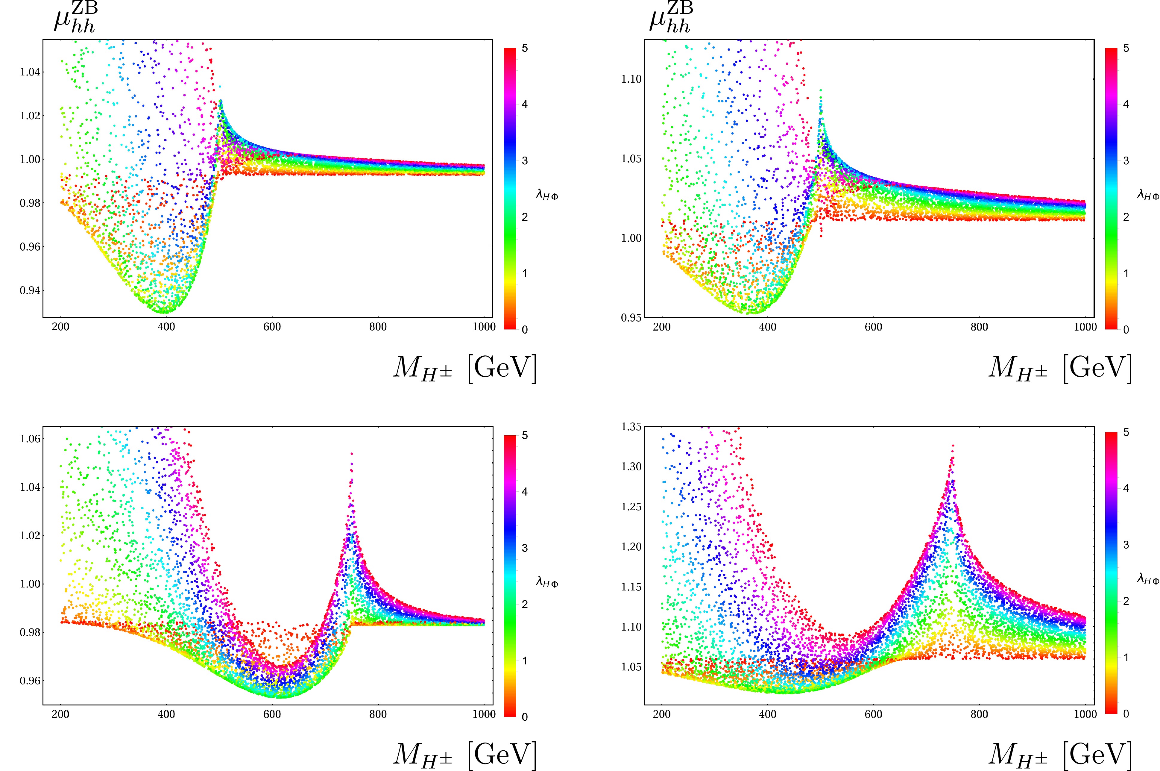

Figure 8

Figure 8. The scatter plots as functions of

$(M_{H^\pm}^2, \lambda_{H\Phi})$ . In these plots, we vary

$200$ GeV

$\leq M_{H^\pm} \leq 1000$ GeV and

$0\leq \lambda_{H\Phi}\leq 5$ .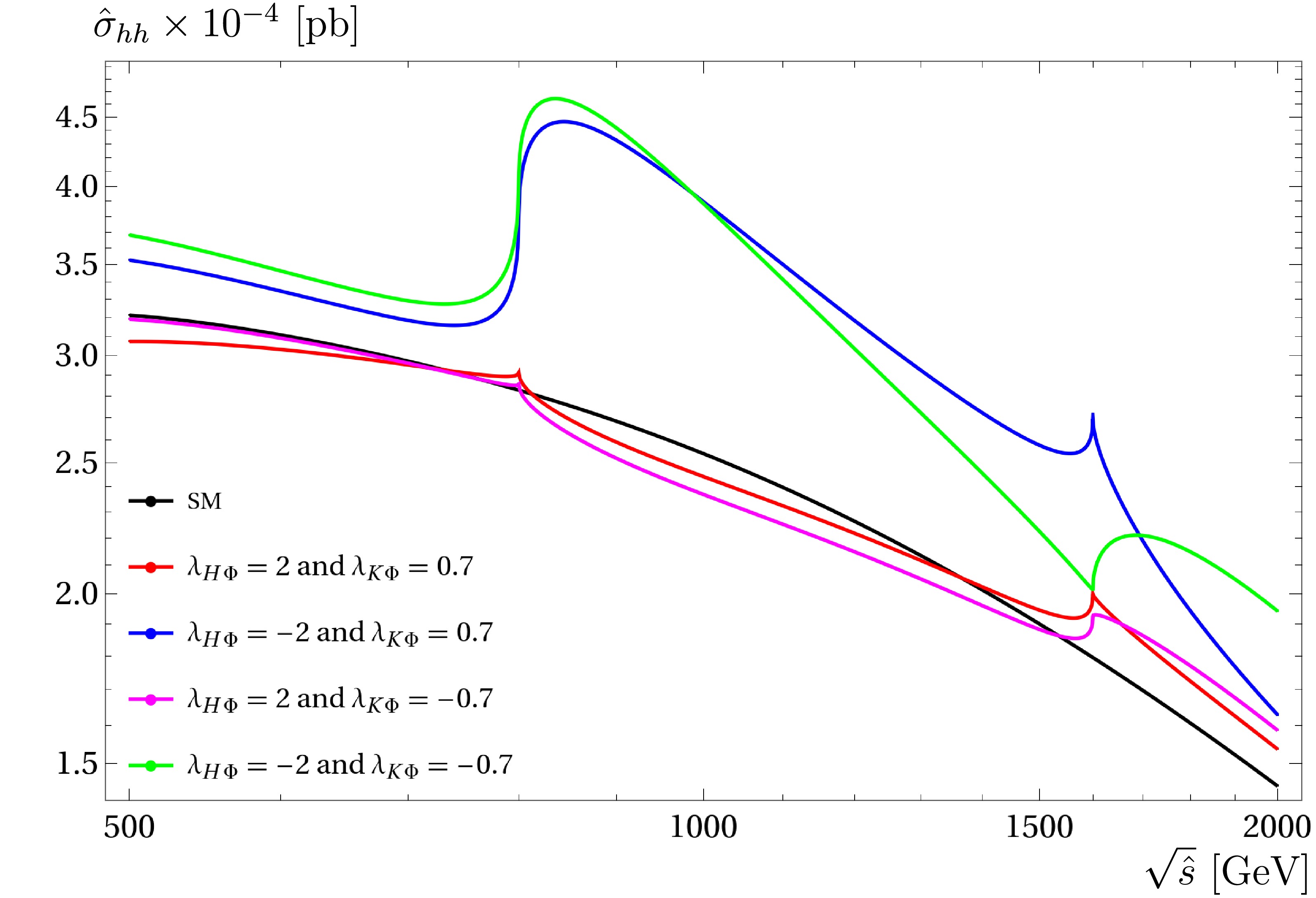

DownLoad: Full-Size Img PowerPoint

Figure 9

Figure 9. Cross section as functions of C.o.M.

$M_{H^\pm} = 400$ GeV,

$M_{K^{\pm\pm}} =800$ GeV and

$\lambda_{K\Phi}=\pm 0.7,~\lambda_{H\Phi}=\pm 2$ . In the following plots, we vary

$\sqrt{\hat{s}} =500$ GeV to

$\sqrt{\hat{s}} =2$ TeV.

DownLoad: Full-Size Img PowerPoint

The investigations for the enhancement factors in the parameter space of $(M_{H^\pm},\; M_{K^{\pm\pm}})$ are next considered. For this study, we take $\lambda_{K\Phi} = \lambda_{H\Phi} = \pm 0.7$ . In the following plots, we vary $200$ GeV $\leq M_{H^\pm},\; M_{K^{\pm\pm}} \leq 1000$ GeV at fixing $\sqrt{\hat{s}} = 1$ TeV (for all plots 10) and $\sqrt{\hat{s}} = 1.5$ TeV (for all plots 11). In general, the factors are inversly propotional to $M_{H^\pm},\; M_{K^{\pm\pm}}$ . For the cases of $\lambda_{H\Phi} = \mp 0.7$ , $\lambda_{K\Phi} = - 0.7$ (for left pannel Figures) the enhancement are domimant at low mass regions of $M_{H^\pm},\; M_{K^{\pm\pm}}$ . We have no peak of the factor around 500 GeV in this case. The factors tend to 1 beyond the regions of $M_{K^{\pm\pm}}> 500$ GeV. We next coments on the cases of $\lambda_{H\Phi} = \mp 0.7$ , $\lambda_{K\Phi} = + 0.7$ (for right pannel Figures), the factors are suppressed in the low mass regions of $M_{H^\pm},\; M_{K^{\pm\pm}}$ . They develop to the peak $2M_{K^{\pm\pm}} = 2M_{H^\pm} = 500$ GeV. The factors are in the range of $[\sim 1.0, \sim 1.15]$ beyond the peak regions.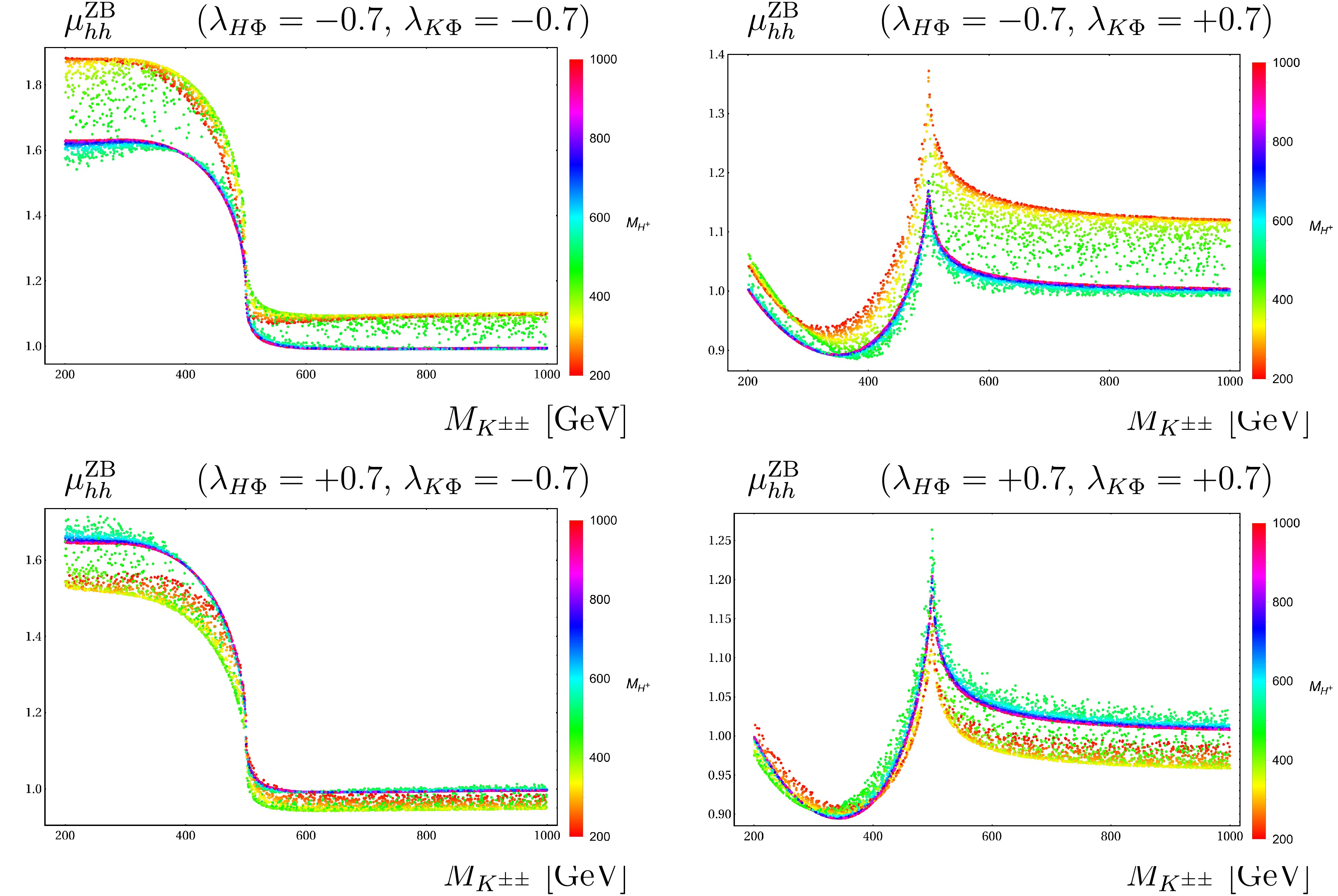

Figure 10

Figure 10. The scatter plots as functions of

$(M_{H^\pm},~M_{K^{\pm\pm}})$ at

$1$ TeV of CoM. In these plots, we vary

$200$ GeV

$\leq M_{H^\pm},~M_{K^{\pm\pm}} \leq 1000$ GeV.

DownLoad: Full-Size Img PowerPoint

The enhancement factors are examined in the parameter space of $(M_{H^\pm},\; M_{K^{\pm\pm}})$ at $1.5$ TeV of CoM. We observe the same behavior of the factors as previous 1 TeV of CoM. In both CoM energies mentioned, the factors in the case of $(\lambda_{H\Phi} = + 0.7$ , $\lambda_{K\Phi} = + 0.7)$ are smallest in comparison with other cases. It is explained as the data in Fig. 9.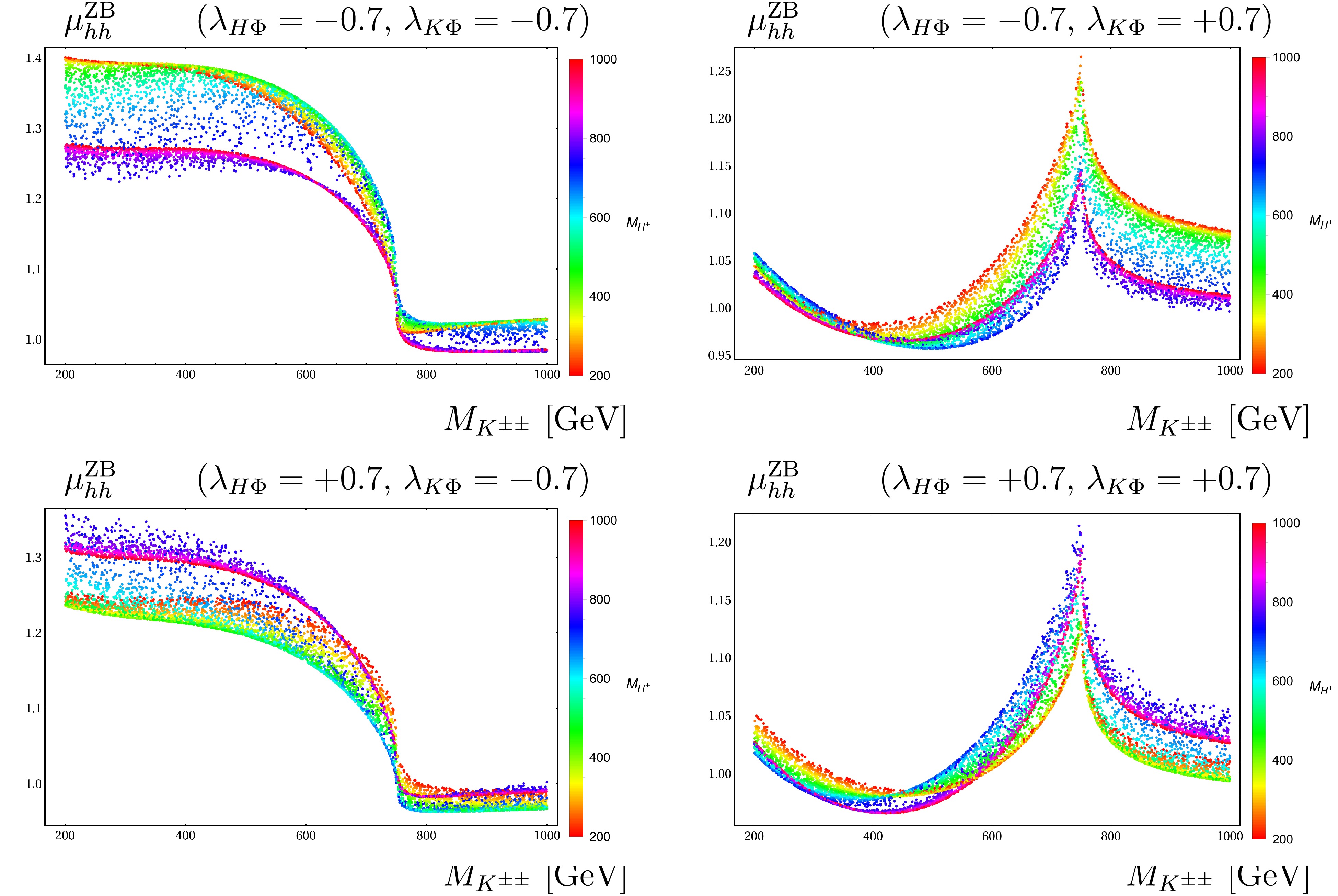

Figure 11

Figure 11. The scatter plots as functions of

$(M_{H^\pm},~M_{K^{\pm\pm}})$ at

$1.5$ TeV of CoM. In these plots, we vary

$200$ GeV

$\leq M_{H^\pm},~M_{K^{\pm\pm}} \leq 1000$ GeV.

DownLoad: Full-Size Img PowerPoint

As we mentioned in the introduction of the paper, by the convolution of the partonic processes in this work with the photon energy spectrum in lepton beams or with the parton distribution functions for initial gluons. Subsequently, we can obtain the corresponding cross-sections for scalar boson pair productions at future colliders including multi-TeV muon collider or the HL-LHC in many of HESMs. These topics are far from our current discussions and will be devoted in our future papers.

IV. CONCLUSIONS

I. INTRODUCTION
II. ONE-LOOP CONTRIBUTIONS FOR PROCESSES $gg/\gamma\gamma \rightarrow \phi_i\phi_j$ IN THE HESMs
Ⅲ. APPLICATIONS
     A Numerical tests
     B Standard model
     C Zee-Babu model
IV. CONCLUSIONS
APPENDIX A: TENSOR REDUCTION FOR ONE-LOOP INTEGRALS
APPENDIX B: ANALYTIC RESULTS FOR ONE-LOOP FORM FACTORS
APPENDIX C: LAGRANGIAN FOR ZEE-BABU MODELS

A general one-loop formulas for loop-induced processes $gg/\gamma \gamma\rightarrow \phi_i\phi_j$ with CP-even Higges $\phi_i,\phi_j = h,\; H_j$ which are valid for a class of Higgs Extensions of the Standard Models, e.g. Inert Doublet Higgs Models, Two Higgs Doublet Models, Zee-Babu models as well as Triplet Higgs Models, etc, are presented in the paper. Analytic expressions for one-loop form factors are written in terms of the basic scalar one-loop functions. The scalar functions are output in the packages ${\tt LoopTools}$ and ${\tt Collier}$ . Physical results are hence evaluated numerically by using one of the mentioned packages. Analytic results are tested by several checks such as the ultraviolet finiteness, infrared finiteness of the one-loop amplitudes. Furthermore, the amplitudes also obey the ward identity due to massless gauge bosons in the initial states. This identity is also verified numerically in the works. Additionally, both the packages ${\tt LoopTools}$ and ${\tt Collier}$ are used for cross-checking for the final results before generating physical results. In the applications, we show phenomenological results for the studied processes in the Zee-Babu model as a typical example in this reference. Production cross-section for the processes $\gamma \gamma\rightarrow hh$ scanned over the masses of singly charged Higgs, doubly charged Higges as well as their couplings to SM-like Higgs are studied.

APPENDIX A: TENSOR REDUCTION FOR ONE-LOOP INTEGRALS

I. INTRODUCTION
II. ONE-LOOP CONTRIBUTIONS FOR PROCESSES $gg/\gamma\gamma \rightarrow \phi_i\phi_j$ IN THE HESMs
Ⅲ. APPLICATIONS
     A Numerical tests
     B Standard model
     C Zee-Babu model
IV. CONCLUSIONS
APPENDIX A: TENSOR REDUCTION FOR ONE-LOOP INTEGRALS
APPENDIX B: ANALYTIC RESULTS FOR ONE-LOOP FORM FACTORS
APPENDIX C: LAGRANGIAN FOR ZEE-BABU MODELS

We apply tensor reduction method developed in Ref. [101] for this computation. The method is described briefly in the appendix. Following the technique, tensor one-loop integrals rank P with N-external legs can be decomposed into the basic scalar one-loop functions with $N\leq 4$ (they are labeled as $A_0$ , $B_0$ , $C_0$ , $D_0$ ). Definition of tensor integrals with rank P (taking $N\leq 4$ external legs for examples) is

$\begin{aligned}[b] \{A; B; C; D\}^{\mu_1\mu_2\cdots \mu_P} = \;&(\mu^2)^{2-d/2} \int \frac{d^dk}{(2\pi)^d} \\& \dfrac{k^{\mu_1}k^{\mu_2}\cdots k^{\mu_P}}{\{D_1;\; D_1 D_2;\; D_1D_2D_3; \; D_1D_2D_3D_4\}}. \end{aligned}$

(A1)

In this formula, $D_j$ ( $j = 1,\cdots, 4$ ) are the inverse Feynman propagators

$D_j = (k+ q_j)^2 -m_j^2 +i\rho,$

(A2)

$q_j = \displaystyle\sum\limits_{i = 1}^j p_i$ , $p_i$ are the external momenta, $m_j$ are internal masses in the loops. One-loop integrals are handled in the space-time dimension $d = 4-2\varepsilon$ . We note that one-loop integrals contain the ultraviolet divergences. The divergent part is as $C_{UV} = 1/\varepsilon - \log(4\pi) +\gamma_E$ with EulerGamma $\gamma_E\sim 0.57721\cdots$ . Furthermore, the fictitious mass λ is introduced for virtual photon to regularize the infrared divergences. The parameter $\mu^2$ plays a key role of a renormalization scale. Explicit reduction formulas for one-loop one-, two-, three- and four-point tensor integrals up to rank $P = 3$ [101] are presented as follows. For one-loop one-, two-, three-point tensor integrals, one has

$A^{\mu} = 0,$

(A3)

$A^{\mu\nu} = g^{\mu\nu} A_{00},$

(A4)

$A^{\mu\nu\rho} = 0,$

(A5)

$B^{\mu} = q^{\mu} B_1,$

(A6)

$B^{\mu\nu} = g^{\mu\nu} B_{00} + q^{\mu}q^{\nu} B_{11},$

(A7)

$B^{\mu\nu\rho} = \{g, q\}^{\mu\nu\rho} B_{001} + q^{\mu}q^{\nu}q^{\rho} B_{111},$

(A8)

and

$C^{\mu} = q_1^{\mu} C_1 + q_2^{\mu} C_2 = \sum\limits_{i = 1}^2q_i^{\mu} C_i,$

(A9)

$C^{\mu\nu} = g^{\mu\nu} C_{00} + \sum\limits_{i,j = 1}^2q_i^{\mu}q_j^{\nu} C_{ij},$

(A10)

$C^{\mu\nu\rho} = \sum\limits_{i = 1}^2 \{g,q_i\}^{\mu\nu\rho} C_{00i}+ \sum\limits_{i,j,k = 1}^2 q^{\mu}_i q^{\nu}_j q^{\rho}_k C_{ijk}.$

(A11)

For one-loop four-point tensor functions, the reduction formulas are given

$D^{\mu} = q_1^{\mu} D_1 + q_2^{\mu} D_2 + q_3^{\mu}D_3 = \sum\limits_{i = 1}^3q_i^{\mu} D_i,$

(A12)

$D^{\mu\nu} = g^{\mu\nu} D_{00} + \sum\limits_{i,j = 1}^3q_i^{\mu}q_j^{\nu} D_{ij},$

(A13)

$D^{\mu\nu\rho} = \sum\limits_{i = 1}^3 \{g,q_i\}^{\mu\nu\rho} D_{00i}+ \sum\limits_{i,j,k = 1}^3 q^{\mu}_i q^{\nu}_j q^{\rho}_k D_{ijk}.$

(A14)

The tensor $\{g, q_i\}^{\mu\nu\rho}$ [101] is given by $\{g, q_i\}^{\mu\nu\rho} = g^{\mu\nu} q^{\rho}_i + g^{\nu\rho} q^{\mu}_i + g^{\mu\rho} q^{\nu}_i$ . The scalar Passarino-Veltman functions (PV-functions) [101] are $A_{00}, B_1, \cdots, D_{333}$ in the right hand sides. The PV-functions are calculated in terms of the basic scalar one-loop functions with $N\leq 4$ , e.g. $A_0$ -, $B_0$ -, $C_0$ - and $D_0$ - scalar functions which are implemented into ${\tt LoopTools}$ [102] and ${\tt Collier}$ [103] for numerical computations.

APPENDIX B: ANALYTIC RESULTS FOR ONE-LOOP FORM FACTORS

I. INTRODUCTION
II. ONE-LOOP CONTRIBUTIONS FOR PROCESSES $gg/\gamma\gamma \rightarrow \phi_i\phi_j$ IN THE HESMs
Ⅲ. APPLICATIONS
     A Numerical tests
     B Standard model
     C Zee-Babu model
IV. CONCLUSIONS
APPENDIX A: TENSOR REDUCTION FOR ONE-LOOP INTEGRALS
APPENDIX B: ANALYTIC RESULTS FOR ONE-LOOP FORM FACTORS
APPENDIX C: LAGRANGIAN FOR ZEE-BABU MODELS

In this appendix, we show analytic results for one-loop form factors given in the equations 11, 12. In the analytic expressions, we use the following kinematic variables as

$x_{t(u)} = \dfrac{\hat{t}(\hat{u})}{\hat{s} }, \quad x_{\phi_{i,j,k}} = \dfrac{M_{\phi_{i,j,k}}^2 } {\hat{s} },$

(B1)

$x_{f} = \dfrac{m_f^2}{\hat{s}}, \quad x_{W} = \dfrac{M_W^2} {\hat{s} }, \quad x_{S} = \dfrac{M_S^2}{\hat{s} }$

(B2)

for $S\equiv S^Q \equiv H^{\pm}$ , $K^{\pm\pm}$ in the below results. We first arrive at the factors $F_{12,f/W/S}^{\text{Trig}}$ calculated from one-loop triangle with connecting to $\phi_k^*$ -poles. The factors are written in terms of scalar one-loop three-point functions $C_0$ . We first take into account all fermions propagating in the loop, as ploted in Fig. 1 ( $G_1$ ), the factors are given explicitly

$F_{12,f}^{\text{Trig}} = \dfrac{1 }{4 \pi ^2} \Big[ 4 x_f + 2 m_f^2 \big( 4 x_f-1 \big) C_0(0,\hat{s},0; m_f^2,m_f^2,m_f^2) \Big].$

(B3)

One next considers one-loop diagrams with W boson exchanged in the loop in connecting with $\phi_k^*$ -poles ( $G_2$ ), as shown in Fig. 1. The corresponding factors are given by

$\begin{aligned}[b] F_{12,W}^{\text{Trig}} = \;&\dfrac{e^2}{8\pi^2\; M_W^2} \Big[ x_{\phi_k} + 6 x_W + 2M_W^2 \big( x_{\phi_k} + 6 x_W - 4 \big) \\& C_0(0,\hat{s},0;M_W^2,M_W^2,M_W^2) \Big]. \end{aligned}$

(B4)

Furthermore, considering singly (as well as doubly) charged Higgses in the loop, as plotted in Fig. 1 ( $G_3$ ), the respective factors are collected as

$F_{12,S}^{\text{Trig}} = - \dfrac{ e^2 Q_S^2 }{4 \pi ^2 \; \hat{s} } \Big[ 1 + 2 M_S^2 \, C_0(0,\hat{s},0; M_S^2,M_S^2,M_S^2) \Big].$

(B5)

Here we note $Q_S$ for charged quantum numbers for charged scalars (S).

We then arrive at the factors contributing from the one-loop box diagrams with fermions f, W-bosons and singly (doubly) charged Higgses S internal lines, noted as $F_{ab, P}^{\text{Box}}$ with $ab \equiv 12, 33$ and $P = f,\; W,\; S$ . For all fermions propagating in the loop, the factors are casted into the form of

$\begin{array}{l} F_{ab,f}^{\text{Box}} = \dfrac{1}{4 \pi ^2} \Bigg[ \delta_{ab}^f + \eta_{ab,f}^{(0)} \cdot C_0(0,\hat{s},0; m_f^2,m_f^2,m_f^2) \\ \;\;\;\;\;\;\;\;\;\;\;\;\;\;\;\; + \eta_{ab,f}^{(1)} \cdot C_0(M_{\phi_i}^2,M_{\phi_j}^2, \hat{s};m_f^2,m_f^2,m_f^2) \\ \;\;\;\;\;\;\;\;\;\;\;\;\;\;\;\; + \eta_{ab,f}^{(2)} \cdot C_0(\hat{t},M_{\phi_i}^2,0 ;m_f^2,m_f^2,m_f^2) \\ \;\;\;\;\;\;\;\;\;\;\;\;\;\;\;\; + \eta_{ab,f}^{(3)} \cdot C_0(M_{\phi_i}^2,0, \hat{u};m_f^2,m_f^2,m_f^2) \\ \;\;\;\;\;\;\;\;\;\;\;\;\;\;\;\; + \eta_{ab,f}^{(4)} \cdot C_0(0,M_{\phi_j}^2,\hat{t} ;m_f^2,m_f^2,m_f^2) \\ \;\;\;\;\;\;\;\;\;\;\;\;\;\;\;\; + \eta_{ab,f}^{(5)} \cdot C_0(\hat{u},M_{\phi_j}^2,0 ;m_f^2,m_f^2,m_f^2) \\ \;\;\;\;\;\;\;\;\;\;\;\;\;\;\;\; + \zeta_{ab,f}^{(0)} \cdot D_0(0,M_{\phi_j}^2,M_{\phi_i}^2,0 ;\hat{t},\hat{s}; m_f^2,m_f^2,m_f^2,m_f^2) \\ \;\;\;\;\;\;\;\;\;\;\;\;\;\;\;\; + \zeta_{ab,f}^{(1)} \cdot D_0(0,M_{\phi_i}^2,M_{\phi_j}^2,0 ;\hat{u},\hat{s}; m_f^2,m_f^2,m_f^2,m_f^2) \\ \;\;\;\;\;\;\;\;\;\;\;\;\;\;\;\; + \zeta_{ab,f}^{(2)} \cdot D_0(M_{\phi_i}^2,0,M_{\phi_j}^2,0 ;\hat{u},\hat{t}; m_f^2,m_f^2,m_f^2,m_f^2) \Bigg]. \end{array}$

(B6)

In this formulas, we have used the notations: $\delta_{12}^f = 4 x_f$ , $\delta_{33}^f = 0$ . All presented coefficients in the above-mentioned factors are given by

$\begin{aligned}[b] \eta_{12,f}^{(0)} =\;& \dfrac{ m_f^2 }{ \Big[ (x_{\phi_i}-x_t) (x_{\phi_j}-x_t) +x_t \Big]^2 } \\ & \times \Bigg\{ 2 x_{\phi_i}^2 \Big[ 4 x_f [ 1 + (x_{\phi_j}-x_t)^2 ] -2 x_{\phi_j}+x_t+1 \Big] \\& + 8 x_t^2 x_f ( 1-x_{\phi_j}+x_t )^2 - x_{\phi_i}^3 \\ & + x_{\phi_i} \Big[ 2 x_t^2 [ 8 x_f (2 x_{\phi_j} - x_t - 1) - 1 ] + (1 - x_{\phi_j}) \\& \big( 16 x_{\phi_j} x_t x_f - 8 x_f - 2 x_t + x_{\phi_j} - 1 \big) \Big] \Bigg\}, \end{aligned}$

(B7)

$\eta_{12,f}^{(1)} = \dfrac{ m_f^2 \; x_{\phi_i} \big( x_{\phi_i}+x_{\phi_j}- 8 x_f-1 \big) \Big[ x_{\phi_i}^2 + x_{\phi_j}^2 + 1 + 2 (x_t + 1) \big( x_t - x_{\phi_i} - x_{\phi_j} \big) \Big] }{\Big[ (x_{\phi_i}-x_t) (x_{\phi_j}-x_t) + x_t \Big]^2},$

(B8)

$\begin{aligned}[b] \eta_{12,f}^{(2)} =& \dfrac{ m_f^2 \; (x_{\phi_i}-x_t)^2 }{\Big[ (x_{\phi_i}-x_t) (x_{\phi_j}-x_t) + x_t \Big]^2} \times \Bigg\{ (8 x_f-x_{\phi_i}-x_{\phi_j}) \Big[ x_t^2 (x_{\phi_i}+2 x_{\phi_j} - x_t - 2) + x_{\phi_i} x_{\phi_j}^2 \Big] + x_t \Big[ (2 x_{\phi_i} +x_{\phi_j}-2) \\& \big[ x_{\phi_j} (x_{\phi_i}+x_{\phi_j}) - 8 x_f x_{\phi_j} \big] - 8 x_f + x_{\phi_j} \Big] + x_{\phi_i} x_{\phi_j} \Bigg\}. \end{aligned}$

(B9)

We also have the following coefficients:

$\begin{aligned}[b] \zeta_{12,f}^{(0)} = \;& \dfrac{ \hat{s}^2 \; x_f } { \Big[ (x_{\phi_i} - x_t) (x_{\phi_j} - x_t) + x_t \Big]^2} \Bigg\{ 16 x_f^2 \Big[ (x_{\phi_i}-x_t) (x_{\phi_j}-x_t) +x_t \Big] \times \Big[ x_{\phi_i} (x_{\phi_j} + 1) - x_t (x_{\phi_i}+x_{\phi_j} - x_t - 1) \Big] \\& +2 x_f \Big\{ -x_{\phi_i}^2 x_{\phi_j} \Big[ x_{\phi_j} (x_{\phi_i}+x_{\phi_j}+2) + x_{\phi_i} - 1 \Big] + x_t^3 (x_{\phi_i}+x_{\phi_j}+1) \Big[ - x_t + 2 \big( x_{\phi_i} +x_{\phi_j}-1 \big) \Big] \\& -x_t^2 \Big[ x_{\phi_i} \big[ x_{\phi_j} \big( 5 x_{\phi_i} + 5 x_{\phi_j} + 1 \big) + x_{\phi_i}^2 + 2 \big] +(x_{\phi_j}-1)^2 (x_{\phi_j}+1) \Big] \\& + x_{\phi_i} x_t (x_{\phi_i}+x_{\phi_j}-1) \Big[ x_{\phi_i} (2 x_{\phi_j} + 1) + x_{\phi_j} (2 x_{\phi_j}+3) - 1 \Big] \Big\} + x_{\phi_i} x_t \big( x_{\phi_i} x_{\phi_j}+x_t^2 \big) \Bigg\}, \end{aligned}$

(B10)

$\begin{aligned}[b] \zeta_{12,f}^{(2)} =\;& \dfrac{ \hat{s}^2 \, x_f }{\Big[ (x_{\phi_i}-x_t) (x_{\phi_j}-x_t) + x_t \Big]} \Bigg\{ 16 x_f^2 \Big[ -x_t (x_{\phi_i}+x_{\phi_j}-x_t-1) + x_{\phi_i} (x_{\phi_j}+1) \Big] -2 x_f \Big\{ x_t^2 \Big[ 4 \big( x_{\phi_i}^2+x_{\phi_j}^2 \big) \\ & - 7 \big( x_{\phi_i}+x_{\phi_j} \big) + 16 x_{\phi_i} x_{\phi_j} + 5 \Big] + x_{\phi_i} \Big[ x_{\phi_i} \big( 4 x_{\phi_j}^2+x_{\phi_j}+1 \big) + x_{\phi_j} (x_{\phi_j}+2)-1 \Big] -x_t (x_{\phi_i}+x_{\phi_j}-1) \\ & \Big[ x_{\phi_i} \big( 8 x_{\phi_j} + 1 \big) + x_{\phi_j} + 1 \Big] + 4 x_t^3 \big[ x_t - 2 (x_{\phi_i} + x_{\phi_j} -1 ) \big] \Big\} + (x_{\phi_i}+x_{\phi_j}) \Big[ (x_{\phi_i}-x_t) (x_{\phi_j}-x_t) + x_t \Big]^2 \Bigg\}. \end{aligned}$

(B11)

The corresponding coefficients for the factors $F_{33,f}^{\text{Box}}$ are shown as follows:

$\begin{aligned}[b] \eta_{33,f}^{(0)} =\; &\dfrac{ m_f^2 }{\Big[ (x_{\phi_i}-x_t) (x_{\phi_j}-x_t) + x_t \Big]^2} \Bigg\{ 8 x_f (x_{\phi_i}+x_{\phi_j}-1) + x_{\phi_i} \big( 2 x_t -4 x_{\phi_j}-x_{\phi_i} + 2 \big) + 2 x_t (x_{\phi_j}-x_t-1) - (x_{\phi_j}-1)^2 \Bigg\}, \end{aligned}$

(B12)

$\eta_{33,f}^{(1)} = \dfrac{1}{x_{\phi_i}} \times \eta_{12,f}^{(1)},$

(B13)

$\eta_{33,f}^{(2)} = \dfrac{ m_f^2 \; \big( x_{\phi_i}-x_t \big) \Big[ x_t \big(x_t-8 x_f \big) + x_{\phi_i} x_{\phi_j} \Big] }{\Big[ (x_{\phi_i}-x_t) (x_{\phi_j}-x_t) + x_t \Big]^2},$

(B14)

$\begin{aligned}[b] \zeta_{33,f}^{(0)} =\;& \dfrac{ s^2 \, x_f }{\Big[ (x_{\phi_i}-x_t) (x_{\phi_j}-x_t) + x_t \Big]^2} \times \Bigg\{ 16 x_f^2 \Big[ (x_{\phi_i}-x_t) (x_{\phi_j}-x_t) + x_t \Big] + x_t \big( x_{\phi_i} x_{\phi_j} + x_t^2 \big) +2 x_f \Big[ -x_t^2 (x_{\phi_i}+x_{\phi_j}+3)\\& + \big[ x_t (x_{\phi_i}+x_{\phi_j}-1) - x_{\phi_i} x_{\phi_j} \big] (x_{\phi_i}+x_{\phi_j}-1) \Big] \Bigg\}, \end{aligned}$

(B15)

and also have

$\zeta_{33,f}^{(2)} = \dfrac{ 2m_f^4 \; \big( 8 x_f-x_{\phi_i}-x_{\phi_j}+1 \big) }{\Big[ (x_{\phi_i}-x_t) (x_{\phi_j}-x_t) + x_t \Big]}.$

(B16)

We next consider one-loop box diagrams with vector boson $W$ in the loop. The factors are then presented as follows:

$\begin{aligned}[b] F_{ab,W}^{\text{Box},1} =\;& \dfrac{e^2}{(4 \pi)^2} \dfrac{1}{ M_W^2 } \Bigg\{ \delta_{ab}^W + \varepsilon_{ab}^W \Big[ B_0(\hat{s}; M_W^2,M_W^2) - B_0(0; M_W^2,M_W^2) \Big] + \eta_{ab,W}^{(0)} \cdot C_0(0,\hat{s},0; M_W^2,M_W^2,M_W^2) + \eta_{ab,W}^{(1)} \\& \cdot C_0(M_{\phi_i}^2, M_{\phi_j}^2,\hat{s}; M_W^2,M_W^2,M_W^2) + \eta_{ab,W}^{(2)} \cdot C_0(\hat{t},M_{\phi_i}^2,0; M_W^2,M_W^2,M_W^2) + \eta_{ab,W}^{(3)} \\&\cdot C_0(M_{\phi_i}^2,0,\hat{u}; M_W^2,M_W^2,M_W^2) + \eta_{ab,W}^{(4)} \cdot C_0(0,M_{\phi_j}^2,\hat{t}; M_W^2,M_W^2,M_W^2) + \eta_{ab,W}^{(5)} \cdot C_0(\hat{u},M_{\phi_j}^2,0; M_W^2,M_W^2,M_W^2) \\& + \zeta_{ab,W}^{(0)} \cdot D_0(0,M_{\phi_j}^2,M_{\phi_i}^2,0 ;\hat{t},\hat{s}; M_W^2,M_W^2,M_W^2,M_W^2) + \zeta_{ab,W}^{(1)} \cdot D_0(0,M_{\phi_i}^2,M_{\phi_j}^2,0 ;\hat{u},\hat{s}; M_W^2,M_W^2,M_W^2,M_W^2) \\ &+ \zeta_{ab,W}^{(2)} \cdot D_0(M_{\phi_i}^2,0,M_{\phi_j}^2,0 ;\hat{u},\hat{t}; M_W^2,M_W^2,M_W^2,M_W^2) \Bigg\}, \end{aligned}$

(B17)

$\begin{array}{l} F_{12,W}^{\text{Box, 2}} = \dfrac{e^2}{(4\pi)^2} \dfrac{2}{\hat{s} } \Bigg\{ 5 +2 \Big[ B_0(\hat{s},M_W^2,M_W^2) - B_0(0,M_W^2,M_W^2) \Big] + 2 \hat{s} \big( 5 x_W - 2 \big) C_0(0,\hat{s},0,M_W^2,M_W^2,M_W^2) \Bigg\}, \end{array}$

(B18)

$F_{12,W}^{\text{Box, 3}} = -\dfrac{e^2}{(4\pi)^2} \dfrac{4}{\hat{s}} \Bigg[ 1 + 2 x_W \; \hat{s} \; C_0(0,\hat{s},0; M_W^2,M_W^2,M_W^2) \Bigg].$

(B19)

Where we definded the following functions as: $\varepsilon_{12}^W = \dfrac{2}{\hat{s} }$ , $\delta_{12}^W = - \dfrac{1}{\hat{s} }$ , $\varepsilon_{33}^W = 0$ , $\delta_{33}^W = 0$ . All coefficients involed with one-loop form factors calculated from the $W$ -boson box diagrams contributions. The coefficients are given explicitly as follows:

$\begin{aligned}[b] \eta_{12,W}^{(0)} =\;& \dfrac{1}{x_W \Big[ (x_{\phi_i}-x_t) (x_{\phi_j}-x_t) + x_t \Big]^2} \times \Bigg\{ - 2 x_t^2 x_W \big(x_W+2\big) \big(1 -x_{\phi_j}+x_t \big)^2 + x_{\phi_i}^2 \Big\{ x_{\phi_j} - x_{\phi_j}^2 \Big[ 2 x_W \big(x_W+2 \big) + 1 \Big]\\& + 4 x_{\phi_j} x_W \Big[ x_t \big(x_W+2 \big) + 3 \Big] - 2 x_W \Big[ x_t \big( 2 x_t +4 \big) + \big( x_t^2 + 6 \big) x_W + 3 \Big] \Big\} + 2 x_{\phi_i} x_W \Big\{ x_{\phi_j}^2 \Big[ 2 x_t \big(x_W+2 \big) + 1 \Big] \\ & - x_{\phi_j} \Big[ 2 x_t \big( 2 x_t x_W + 4 x_t+x_W+4 \big) +6 x_W+3 \Big] + 2 x_t \big(x_t+1\big) \Big[ x_t \big(x_W+2\big) +2 \Big] +6 x_W+2 \Big\} - x_{\phi_i}^3 \big( x_{\phi_j} - 2 x_W \big) \Bigg\}, \end{aligned}$

(B20)

$\begin{array}{l} \eta_{12,W}^{(1)} = \dfrac{ x_{\phi_i} } { x_W \Big[ (x_{\phi_i}-x_t) (x_{\phi_j}-x_t) + x_t \Big]^2 } \times \Big[ x_{\phi_i} x_{\phi_j} - 2 x_W (x_{\phi_i}+x_{\phi_j}-6 x_W-2) \Big] \times \Big[ x_{\phi_i}^2 + x_{\phi_j}^2 + 1 + 2 \big( x_t - x_{\phi_i} - x_{\phi_j} \big) \big( x_t+1 \big) \Big], \end{array}$

(B21)

$\begin{aligned}[b] \eta_{12,W}^{(2)} =\;& - \dfrac{ (x_{\phi_i}-x_t)^2 }{ x_W \Big[ (x_{\phi_i}-x_t) (x_{\phi_j}-x_t) + x_t \Big]^2 } \times \Bigg\{ x_{\phi_i} \big( x_{\phi_j}-x_t \big)^2 \Big[ x_{\phi_i} \big( x_{\phi_j}-2 x_W \big) + 12 x_W^2 \Big] -2 x_{\phi_i} x_W \Big[ x_{\phi_j} \big(x_{\phi_j}^2 + 2 x_t -2 \big) \\& - x_t^2 \big( x_t - 3 x_{\phi_j} + 2 \big) + x_t \big( 1 - 3 x_{\phi_j}^2 \big) \Big] + x_t \big( 1-x_{\phi_j}+x_t \big)^2 \Big[ 2 x_W \big( x_{\phi_j}-6 x_W \big) - x_{\phi_i} x_{\phi_j} \Big] \Bigg\}. \end{aligned}$

(B22)

All coefficients for scalar one-loop four-point functions in the above-equations are given by

$\begin{aligned}[b] \zeta_{12,W}^{(0)} =\;& \dfrac{ \hat{s} }{x_W \Big[ (x_{\phi_i}-x_t) (x_{\phi_j}-x_t) + x_t \Big]^2} \times \Bigg\{ 2 x_W x_{\phi_i}^3 \big( x_t - x_{\phi_j} \big) \Big[ x_{\phi_j}^2 - x_{\phi_j} \big(x_t+2 x_W+1 \big) + 2 x_W \big(x_t-1 \big) + 2 x_t \Big] \\& + x_{\phi_i}^2 \Big\{ 2 x_t x_W \Big[ x_{\phi_j}^2 \big(2 x_{\phi_j}-5 \big) + 2 x_t^2 \big(x_{\phi_j}-2 \big) + x_{\phi_j} x_t \big(9-4 x_{\phi_j} \big) + x_{\phi_j}-3 x_t \Big] + 4 x_W^2 \Big[ x_t^2 \big(5 x_{\phi_j}+1 \big) \\& + x_t \big( -4 x_{\phi_j}^2 -4 x_{\phi_j} + 3 \big) + x_{\phi_j} \big( x_{\phi_j}^2 + 3 x_{\phi_j} - 2 \big) - 2 x_t^3 \Big] - 24 x_W^3 \big(x_{\phi_j}-x_t \big) \big(x_{\phi_j}-x_t+1 \big) + x_{\phi_j} x_t^2 \Big\} \\& + 2 x_{\phi_i} x_t x_W \Big\{ x_t \Big[ 2 x_{\phi_j}^2 \big(x_t+2 \big) - x_{\phi_j} \big(x_t^2 + 6x_t + 4 \big) + 2 \big(x_t^2+x_t+1\big) - x_{\phi_j}^3 \Big] \\& + 2 x_W \Big[ x_t^3 - 2 x_t - 2 - 2 x_t^2 \big(2 x_{\phi_j}+1 \big) + 5 x_{\phi_j} x_t \big(x_{\phi_j}+1 \big) + x_{\phi_j} \big(7- 2 x_{\phi_j}^2 - 3 x_{\phi_j} \big) \Big] \\& + 12 x_W^2 \big(x_{\phi_j}-x_t-1 \big) \big(2 x_{\phi_j} -2 x_t+1 \big) \Big\} + 4 x_t^2 x_W^2 \big(x_{\phi_j}-6 x_W+2 \big) \big(1-x_{\phi_j}+x_t \big)^2 \Bigg\}, \end{aligned}$

(B23)

$\begin{aligned}[b] \zeta_{12,W}^{(2)} =\;& \dfrac{\hat{s} } {x_W \Big[ (x_{\phi_i}-x_t) (x_{\phi_j}-x_t) + x_t \Big]} \Bigg\{ x_{\phi_i}^3 \big(x_{\phi_j}-2 x_W \big) \big(x_{\phi_j}-x_t \big)^2 + 2 x_{\phi_i}^2 \Big\{ 2 x_W^2 \Big[ x_{\phi_j} \big( 3 x_{\phi_j} - 6 x_t + 1 \big) + x_t \big(3 x_t-1 \big) + 1 \Big] \\& - x_W \Big[ x_{\phi_j}^2 \big(x_{\phi_j}-4 x_t+1 \big) + x_{\phi_j} \big(5 x_t^2+x_t-1\big) - 2 x_t \big(x_t^2+x_t-1\big) \Big] \\& - x_{\phi_j} x_t \big(x_{\phi_j}-x_t \big) \big(x_{\phi_j}-x_t-1 \big) \Big\} + x_{\phi_i} \Big\{ -4 x_W^2 \Big[ x_{\phi_j}^2 \big(6 x_t-1 \big) -x_{\phi_j} \big( 12 x_t^2 + 4 x_t + 3 \big) + x_t \big(6 x_t^2 + 5 x_t + 1 \big) + 2 \Big] \\& + 2 x_t x_W \big(x_{\phi_j}-x_t-1 \big) \Big[ x_t \big( x_t + 1 \big) - 2 + x_{\phi_j} \big( 2 x_{\phi_j} - 3 x_t + 1 \big) \Big] + x_{\phi_j} x_t^2 \big(-x_{\phi_j}+x_t+1 \big)^2 - 24 x_W^3 \big(x_{\phi_j}-x_t+1 \big) \Big\} \\& - 2 x_t x_W \big(x_{\phi_j}-x_t-1 \big) \times \Big[ x_t \big(x_{\phi_j}-6 x_W \big) \big( x_{\phi_j} - x_t - 1 \big) + 2 x_W \big(x_{\phi_j}-6 x_W + 2 \big) \Big] \Bigg\}.\end{aligned}$

(B24)

Furthermore, one gives the coefficients appear in the factors $F_{33,W}^{\text{Box}}$

$\begin{aligned}[b] \eta_{33,W}^{(0)} =\;& \dfrac{1}{x_W \Big[ (x_{\phi_i}-x_t) (x_{\phi_j}-x_t) + x_t \Big]^2} \Bigg\{ \big( 12 x_W^2 + x_{\phi_i} x_{\phi_j} \big) \big( 1-x_{\phi_i}-x_{\phi_j} \big) + 2 x_W \Big[ x_{\phi_i} \big( x_{\phi_i} +6 x_{\phi_j}-4 x_t-3 \big)\\& + \big(x_{\phi_j}-2 x_t \big)^2 - 3 x_{\phi_j} + 4 x_t + 2 \Big] \Bigg\}, \end{aligned}$

(B25)

$\eta_{33,W}^{(1)} = \dfrac{1}{x_{\phi_i}} \times \eta_{12,W}^{(1)},$

(B26)

$\eta_{33,W}^{(2)} = \dfrac{\big(x_{\phi_i}-x_t \big) \Big[ x_{\phi_i} x_{\phi_j} \big(x_t-4 x_W \big) + 2 x_t x_W \big(x_{\phi_j} + x_{\phi_i} - 2 x_t+6 x_W \big) \Big] }{ x_W \Big[ (x_{\phi_i}-x_t) (x_{\phi_j}-x_t) + x_t \Big]^2}.$

(B27)

Furthermore, one gives

$\begin{aligned}[b] \zeta_{33,W}^{(0)} = \;&\dfrac{\hat{s} }{x_W \Big[ (x_{\phi_i}-x_t) (x_{\phi_j}-x_t) +x_t \Big]^2} \times \Bigg\{ 2 x_{\phi_i}^2 x_W \big(x_{\phi_j}-x_t \big) \big(x_{\phi_j}-2 x_t+2 x_W \big) + 8 x_W^2 x_{\phi_i} x_t \\& + x_{\phi_i} \Big\{ 4 x_W^2 \Big[ x_{\phi_j}^2 + \big(x_t - 2 x_{\phi_j}\big) \big(x_t+1\big) \Big] + 2 x_t x_W \Big[ x_{\phi_j} \big( - 3 x_{\phi_j} + 7 x_t + 1\big) - x_t \big(4 x_t+3\big) \Big] \\& + 24 x_W^3 \big(x_t-x_{\phi_j}\big) + x_{\phi_j} x_t^2 \Big\} +2 x_t x_W \Big\{ x_t \Big[ x_{\phi_j} \big(2 x_{\phi_j} - 4 x_t - 3\big) + 2 \big(x_t^2+x_t+1\big) \Big] \\& +12 x_W^2 \big(x_{\phi_j}-x_t-1 \big) +2 x_W \Big[ x_{\phi_j} \big(-x_{\phi_j}+x_t+3 \big) + x_t-2 \Big] \Big\} \; \Bigg\},\end{aligned}$

(B28)

$\zeta_{33,W}^{(2)} = \dfrac{2 \hat{s} \Big[ x_{\phi_i} \big( x_{\phi_j} - 2 x_t+2 x_W \big) + 2 x_W \big(x_{\phi_j}-6 x_W-2 \big) + 2 x_t \big( x_t - x_{\phi_j} + 1 \big) \Big] }{\Big[ (x_{\phi_i}-x_t) (x_{\phi_j}-x_t) + x_t \Big]}.$

(B29)

Besides, the remaining factors with a shorted abbreviation like $P \equiv f, W, S$ are directly expressed by the following relations as shown,

$\eta_{ab,P}^{(3)} \equiv \eta_{ab,P}^{(2)} \, \big(x_t \leftrightarrow x_u \big),\;\;\;\;\;\;\;\; \eta_{ab,P}^{(4)} = \dfrac{x_{\phi_j} - x_t}{x_{\phi_i} - x_t} \times \eta_{ab,P}^{(2)},$

(B30)

$\eta_{ab,P}^{(5)} = \dfrac{x_{\phi_j} - x_u}{x_{\phi_i} - x_u} \times \eta_{ab,P}^{(3)},\;\;\;\;\;\;\;\; \zeta_{ab,P}^{(1)} \equiv \zeta_{ab,P}^{(0)} \, \big(x_t \leftrightarrow x_u \big).$

(B31)

We pay attention to the contributions of singly (doubly) charged Higges exchanging in the loop. The factors are given by

$\begin{aligned}[b] F_{ab,S}^{\text{Box}, 1} =\;& \dfrac{ e^2 Q_S^2 }{4 \pi ^2} \Bigg\{ \eta_{ab,S}^{(0)} \cdot C_0(0,\hat{s},0 ;M_S^2,M_S^2,M_S^2) + \eta_{ab,S}^{(1)} \cdot C_0(M_{\phi_i}^2,M_{\phi_j}^2 ,\hat{s} ;M_S^2,M_S^2,M_S^2) + \eta_{ab,S}^{(2)} \cdot C_0(\hat{t},M_{\phi_i}^2,0 ;M_S^2,M_S^2,M_S^2) \\& + \eta_{ab,S}^{(3)} \cdot C_0(M_{\phi_i}^2,0,\hat{u} ;M_S^2,M_S^2,M_S^2) + \eta_{ab,S}^{(4)} \cdot C_0(0,M_{\phi_j}^2,\hat{t} ;M_S^2,M_S^2,M_S^2) \\& + \eta_{ab,S}^{(5)} \cdot C_0(\hat{u},M_{\phi_j}^2,0 ;M_S^2,M_S^2,M_S^2) + \zeta_{ab,S}^{(0)} \cdot D_0(0,M_{\phi_j}^2,M_{\phi_i}^2,0 ;\hat{t},\hat{s};M_S^2,M_S^2,M_S^2,M_S^2) \\& + \zeta_{ab,S}^{(1)} \cdot D_0(0,M_{\phi_i}^2,M_{\phi_j}^2,0 ;\hat{u},\hat{s};M_S^2,M_S^2,M_S^2,M_S^2) + \zeta_{ab,S}^{(2)} \cdot D_0(M_{\phi_i}^2,0,M_{\phi_j}^2,0 ;\hat{u},\hat{t};M_S^2,M_S^2,M_S^2,M_S^2) \Bigg\}, \end{aligned}$

(B32)

$F_{12,S}^{\text{Box},2} = \dfrac{ e^2 Q_S^2 }{4 \pi ^2} \Big[ -\dfrac{1}{\hat{s} } - 2 x_{S} \, C_0(0,\hat{s},0,M_S^2,M_S^2,M_S^2) \Big].$

(B33)

All coefficients related to the above-formulas are given explicitly

$\eta_{12,S}^{(0)} = -\dfrac{x_{\phi_i} \big( x_{\phi_i}+x_{\phi_j}-1 \big)}{s \Big[\big(x_{\phi_i}-x_t\big) \big(x_{\phi_j}-x_t\big) + x_t \Big]^2},$

(B34)

$\eta_{12,S}^{(1)} = \dfrac{x_{\phi_i} \Big[ x_{\phi_i}^2 + x_{\phi_j}^2 + 2 \big( x_t - x_{\phi_i} - x_{\phi_j} \big) \big( x_t+1 \big) + 1 \Big] }{s \Big[\big(x_{\phi_i}-x_t\big) \big(x_{\phi_j}-x_t\big) + x_t \Big]^2},$

(B35)

$\eta_{12,S}^{(2)} = -\dfrac{(x_{\phi_i}-x_t)^2 \Big[ x_{\phi_i} \big( x_{\phi_j}-x_t \big)^2 - x_t \big( -x_{\phi_j}+x_t+1 \big)^2 \Big] }{s \Big[ \big(x_{\phi_i}-x_t\big) \big(x_{\phi_j}-x_t\big) + x_t \Big]^2}.$

(B36)

The coefficients of scalar one-loop four-point integrals in the above equations are

$\begin{array}{l} \zeta_{12,S}^{(0)} = \dfrac{1}{ \Big[ \big(x_{\phi_i}-x_t\big) \big(x_{\phi_j}-x_t\big) + x_t \Big]^2} \times \Bigg\{ x_{\phi_i} x_t^2 - 2 x_{S} \Big[ \big( x_{\phi_i}-x_t \big) \big( x_{\phi_j}-x_t \big) + x_t \Big] \times \Big[ -x_t \big( x_{\phi_i}+x_{\phi_j} - 1 \big) +x_{\phi_i} \big( x_{\phi_j}+1 \big) + x_t^2 \Big] \Bigg\}, \end{array}$

(B37)

$\begin{array}{l} \zeta_{12,S}^{(2)} = \dfrac{1}{ \Big[ \big(x_{\phi_i}-x_t\big) \big(x_{\phi_j}-x_t\big) + x_t \Big]} \times \Bigg\{ \Big[ \big(x_{\phi_i}-x_t\big) \big(x_{\phi_j}-x_t\big) + x_t \Big]^2 - 2 x_{S} \Big[ -x_t \big(x_{\phi_i}+x_{\phi_j} - 1\big) + x_{\phi_i} \big(x_{\phi_j}+1\big) + x_t^2 \Big] \Bigg\}. \end{array}$

(B38)

Other coefficients are calculated as

$\eta_{33,S}^{(0)} = \dfrac{1}{x_{\phi_i}} \times \eta_{12,S}^{(0)},$

(B39)

$\eta_{33,S}^{(1)} = \dfrac{1}{x_{\phi_i}} \times \eta_{12,S}^{(1)},$

(B40)

$\eta_{33,S}^{(2)} = \dfrac{x_t \big(x_{\phi_i}-x_t\big)}{s \Big[ \big(x_{\phi_i}-x_t\big) \big(x_{\phi_j}-x_t\big) + x_t \Big]^2},$

(B41)

$\zeta_{33,S}^{(0)} = \dfrac{x_t^2-2 x_{S} \Big[ \big(x_{\phi_i}-x_t\big) \big(x_{\phi_j}-x_t\big) + x_t \Big]}{ \Big[\big(x_{\phi_i}-x_t\big) \big(x_{\phi_j}-x_t\big) + x_t \Big]^2},$

(B42)

$\zeta_{33,S}^{(2)} = -\dfrac{2 x_{S}}{ \Big[\big(x_{\phi_i}-x_t\big) \big(x_{\phi_j}-x_t\big) + x_t \Big]}.$

(B43)

We arrive at contributions of mixing charged Higgs $H^\pm$ and vector boson $W^\pm$ boxes diagrams as follows:

$\begin{aligned}[b] F_{ab,W, H^\pm}^{\text{Box}} =\;& \dfrac{e^2}{4 \pi^2} \Bigg\{ \delta_{ab}^{W, H^\pm} + \varepsilon_{ab}^{W, H^\pm} \Big[ B_0(\hat{s},M_W^2,M_W^2) - B_0(0,M_W^2,M_W^2) \Big] + \eta_{ab,W, H^\pm}^{(0)} \cdot C_0(0,\hat{s},0 ;M_W^2,M_W^2,M_W^2) \\& + \eta_{ab,W, H^\pm}^{(1)} \cdot C_0(0,\hat{s},0; M_{H^\pm}^2,M_{H^\pm}^2, M_{H^\pm}^2) + \eta_{ab,W, H^\pm}^{(2)} \cdot \Big[ C_0(M_{\phi_i}^2,\hat{s},M_{\phi_j}^2 ;M_{H^\pm}^2,M_W^2,M_W^2) + C_0(\hat{s},M_{\phi_i}^2,M_{\phi_j}^2 ;M_{H^\pm}^2,M_{H^\pm}^2,M_W^2) \Big] \\& + \eta_{ab,W, H^\pm}^{(3)} \cdot \Big[ C_0(\hat{t},0,M_{\phi_i}^2 ;M_{H^\pm}^2,M_W^2,M_W^2) + C_0(0,\hat{t},M_{\phi_i}^2 ;M_{H^\pm}^2,M_{H^\pm}^2,M_W^2) \Big] + \eta_{ab,W, H^\pm}^{(4)} \cdot \Big[ C_0(\hat{t},0,M_{\phi_j}^2 ;M_{H^\pm}^2,M_W^2,M_W^2) \\& + C_0(0,\hat{t},M_{\phi_j}^2 ;M_{H^\pm}^2,M_{H^\pm}^2,M_W^2) \Big] + \eta_{ab,W, H^\pm}^{(5)} \cdot \Big[ C_0(\hat{u},0,M_{\phi_i}^2 ;M_{H^\pm}^2,M_W^2,M_W^2) \\& + C_0(0,\hat{u},M_{\phi_i}^2 ;M_{H^\pm}^2,M_{H^\pm}^2,M_W^2) \Big] + \eta_{ab,W, H^\pm}^{(6)} \cdot \Big[ C_0(\hat{u},0,M_{\phi_j}^2; M_{H^\pm}^2,M_W^2,M_W^2) \\& + C_0(0,\hat{u},M_{\phi_j}^2; M_{H^\pm}^2,M_{H^\pm}^2,M_W^2) \Big] + \zeta_{ab,W, H^\pm}^{(0)} \cdot D_0(\hat{t},0,\hat{s},M_{\phi_i}^2 ;M_{\phi_j}^2,0; M_{H^\pm}^2,M_W^2,M_W^2,M_W^2) \\& + \zeta_{ab,W, H^\pm}^{(1)} \cdot D_0(\hat{u},0,\hat{s},M_{\phi_j}^2 ;M_{\phi_i}^2,0; M_{H^\pm}^2,M_W^2,M_W^2,M_W^2) + \zeta_{ab,W, H^\pm}^{(2)} \cdot D_0(0,\hat{s},M_{\phi_i}^2,\hat{t} ;0,M_{\phi_j}^2; M_{H^\pm}^2,M_{H^\pm}^2, M_{H^\pm}^2,M_W^2) \\& + \zeta_{ab,W, H^\pm}^{(3)} \cdot D_0(0,\hat{s},M_{\phi_j}^2,\hat{u}; 0,M_{\phi_i}^2; M_{H^\pm}^2,M_{H^\pm}^2, M_{H^\pm}^2,M_W^2) + \zeta_{ab,W, H^\pm}^{(4)} \cdot D_0(0,\hat{u},0,\hat{t} ;M_{\phi_i}^2,M_{\phi_j}^2; M_{H^\pm}^2,M_{H^\pm}^2,M_W^2,M_W^2) \Bigg\}. \end{aligned}$

(B44)

In the above-equations, we have used the following functions as: $\varepsilon_{12}^{W, H^\pm} = 2/\hat{s}$ , $\delta_{12}^{W, H^\pm} = - 1/\hat{s},$ $\varepsilon_{33}^{W, H^\pm} = 0$ and $\delta_{33}^{W, H^\pm} = 0.$ Remaining coefficients relating to the formulas are given

$\begin{aligned}[b] \eta_{12,W, H^\pm}^{(0)} =\;& \dfrac{1}{x_W \Big[ (x_{\phi_i}-x_t) (x_{\phi_j}-x_t) + x_t \Big]^2} \times \Bigg\{ x_{\phi_i} x_W \Big[ 2 x_{H^\pm} \big( x_{\phi_i} +x_{\phi_j}-3 x_{H^\pm}+1 \big) + 4 x_{\phi_i} x_{\phi_j} \big( 2 - x_{\phi_j} \big) + x_{\phi_i} \big( x_{\phi_i} - 3 \big) \\& + x_{\phi_j} \big( x_{\phi_j} - 3 \big) + 2 \Big] - 4 x_t^2 x_W \Big[ x_{\phi_i}^2 + x_t^2 + \big( 4 x_{\phi_i} + x_{\phi_j} - 1 \big) \big( x_{\phi_j}-1 \big) \Big] + 8 x_t x_W \big( x_{\phi_i}+x_{\phi_j}-1 \big) \Big[ x_t^2 + x_{\phi_i} \big( x_{\phi_j}-1 \big) \Big] \\& + x_{\phi_i} x_W^2 \Big[ 4 x_t^2 \big( 2 x_{\phi_j}-x_t-1 \big) + \big( 1 - 4 x_{\phi_j} x_t \big) \big( x_{\phi_j}-1 \big) + 6 x_{H^\pm} - 2 \Big] + x_{\phi_i}^2 x_W^2 \Big[ 1 + 2 \big( x_{\phi_j}-x_t \big)^2 \Big] \\& + 2 x_t^2 x_W^2 \big( x_{\phi_j}-x_t-1 \big)^2 + x_{\phi_i} \Big[ \big( x_{H^\pm}-x_{\phi_i} \big) \big( x_{H^\pm}-x_{\phi_j} \big) \big( 2 x_{H^\pm}-x_{\phi_i}-x_{\phi_j}+1 \big) - 2 x_W^3 \Big] \Bigg\}, \end{aligned}$

(B45)

$\begin{aligned}[b] \eta_{12,W, H^\pm}^{(1)} =\;& \dfrac{1}{x_W \Big[ (x_{\phi_i}-x_t) (x_{\phi_j}-x_t) + x_t \Big]^2} \times \Bigg\{ x_{\phi_i} x_{H^\pm}^2 \big( x_{\phi_i}+x_{\phi_j} -2 x_{H^\pm}+6 x_W+1 \big) \\& + x_{H^\pm} \Big\{ x_{\phi_i}^2 \Big[ x_{\phi_i} + 2 x_W - 1 - 4 x_W \big( x_{\phi_j}-x_t \big)^2 \Big] - 2 x_W \Big[ 3 x_{\phi_i} x_W + 2 x_t^2 \big( x_{\phi_j}-x_t-1 \big)^2 \Big] \\& + 2 x_{\phi_i} x_W \Big[ 4 x_{\phi_j} x_t \big( x_{\phi_j}+2 x_t-1 \big) + 4 x_t^2 \big( x_t+1 \big) - 3 \Big] + x_{\phi_i} x_{\phi_j} \big( x_{\phi_j}+2 x_W-1 \big) \Big\} \\& - x_{\phi_i} \big( x_{\phi_i} + x_{\phi_j} -2 x_W-1 \big) \Big[ x_{\phi_i} x_{\phi_j} - x_W \big( x_{\phi_i} +x_{\phi_j}-x_W-2 \big) \Big] \Bigg\},\end{aligned}$

(B46)

$\begin{aligned}[b] \eta_{12,W, H^\pm}^{(2)} =\;& \dfrac{x_{\phi_i}}{x_W \Big[ (x_{\phi_i}-x_t) (x_{\phi_j}-x_t) + x_t \big]^2} \times \Big[ x_{\phi_i}^2 + x_{\phi_j}^2 + 2 \big(x_t+1 \big) \big(x_t - x_{\phi_i} - x_{\phi_j} \big) + 1 \Big] \\& \times \Big[ x_{\phi_i} x_{\phi_j} - x_{H^\pm} \big( x_{\phi_i} +x_{\phi_j} -x_{H^\pm} +2 x_W \big) - x_W \big( x_{\phi_i} +x_{\phi_j} -x_W -2 \big) \Big], \end{aligned}$

(B47)

$\begin{aligned}[b] \eta_{12,W, H^\pm}^{(3)} =\;& \dfrac{ (x_{\phi_i}-x_t)^2 }{x_W \Big[ (x_{\phi_i}-x_t) (x_{\phi_j}-x_t) + x_t \Big]^2} \times \Bigg\{ x_{H^\pm} \big( x_{\phi_i}+x_{\phi_j} -x_{H^\pm}+2 x_W \big) \Big[ x_{\phi_i} \big( x_{\phi_j}-x_t \big)^2 - x_t \big( x_{\phi_j}-x_t-1 \big)^2 \Big] \\& + x_W x_{\phi_i} \Big[ x_{\phi_j} \big( x_{\phi_j}^2 - 3 x_{\phi_j} x_t + 3 x_t^2 + 2 x_t - 2 \big) - x_t \big( x_t^2 + 2 x_t - 1 \big) \Big] + x_{\phi_j} x_t x_{\phi_i} \big( x_{\phi_j}-x_t-1 \big)^2 - x_W^2 x_{\phi_i} \big( x_{\phi_j}-x_t \big)^2 \\& + \big( x_W-x_{\phi_j} \big) \Big[ x_t x_W \big( x_{\phi_j}-x_t-1 \big)^2 + x_{\phi_i}^2 \big( x_{\phi_j}-x_t \big)^2 \Big] \Bigg\}. \end{aligned}$

(B48)

Other terms are presented as follows:

$\begin{aligned}[b] \zeta_{12,W, H^\pm}^{(0)} =\;& \dfrac{ \hat{s} }{x_W \Big[ (x_{\phi_i}-x_t) (x_{\phi_j}-x_t) + x_t \Big]^2} \times \Bigg\{ x_{\phi_i} x_{H^\pm} \Big[ 2 x_{\phi_i}^2 x_W \big( x_{\phi_j} - x_t \big) \big( x_{\phi_j} - x_t + 1 \big) - x_{H^\pm}^2 \big( x_{\phi_i}+x_{\phi_j} - x_{H^\pm}+2 x_t +4 x_W \big) \Big] \\& - 2 x_{\phi_i}^3 x_W \big( x_{\phi_j}-x_t \big) \Big[ 2 x_t + x_W \big( x_t-1 \big) - x_{\phi_j} \big( x_t+x_W-x_{\phi_j}+1 \big) \Big] + 2 x_W x_t^2 \big( x_{\phi_j}-x_t-1 \big)^2 \Big[ x_W \big( x_{\phi_j}-x_W \big) \\& + x_{H^\pm} \big( x_{\phi_j}+2 x_W-2 \big) \Big] + x_{\phi_i} x_{\phi_j} x_t^2 \big( x_{\phi_i} - x_{H^\pm} \big) + x_{H^\pm}^2 \Big\{ x_{\phi_i}^2 \Big[ x_{\phi_j} + 2 x_t + x_W - 2 x_W \big( x_{\phi_j}-x_t \big) \big( x_{\phi_j}-x_t+1 \big) \Big] \\& + x_{\phi_i} \Big[ x_{\phi_j} x_W \big( 4 x_{\phi_j} x_t + 1 \big) - 2 x_{\phi_j} x_t \big( 4 x_t x_W + x_W-1 \big) + 2 x_W \big( 2 x_t + 1 \big) \big( x_t^2 + 1 \big) + x_t^2 + 6 x_W^2 \Big] - 2 x_t^2 x_W \big( x_{\phi_j}-x_t\\& - 1 \big)^2 \Big\} + x_{\phi_i}^2 x_{H^\pm} \Big\{ 2 x_W \big( x_{\phi_j} - x_t \big) \Big[ x_t \big( 2 x_t - 3 x_{\phi_j} + 3 \big) + x_{\phi_j} \big( x_{\phi_j} - 1 \big) + 1 \Big] + x_W^2 \big( 2 x_{\phi_j} - 2 x_t+1 \big)^2 - x_t \big( 2 x_{\phi_j} +x_t \big) \Big\} \\& + x_{\phi_i} x_{H^\pm} \Big\{ x_W^2 \Big[ x_{\phi_j} - 4 x_W - 2 x_t \big( 4 x_{\phi_j}^2 + 4 x_t^2 + 2 x_t + 1 \big) + 4 x_{\phi_j} x_t \big( 4 x_t+1 \big) - 4 \Big] + 2 x_t x_W \Big[ x_{\phi_j}^2 \big( 5 x_t -2 x_{\phi_j} +5 \big) \\& - x_{\phi_j} \big( 4 x_t^2 +11x_t +5 \big) + x_t \big( x_t^2+6x_t+6 \big) \Big] \Big\} + x_{\phi_i}^2 \Big\{ x_W^3 \Big[ 2 x_t \big( 2 x_{\phi_j}- x_t+1 \big) - 2 x_{\phi_j} \big( x_{\phi_j}+1 \big) - 1 \Big] \\& + x_W^2 \Big[ x_{\phi_j} \big( 2 x_{\phi_j}^2 +2 x_{\phi_j}-7 \big) + 2 x_t^2 \big( 5 x_{\phi_j} - 2 x_t-1 \big) - 8 x_t \big( x_{\phi_j}^2-1 \big) \Big] + x_t x_W \Big[ x_t \big( 18 x_{\phi_j} -8 x_{\phi_j}^2-5 \big) \\& + 2 x_{\phi_j} \big( x_{\phi_j}-2 \big) \big( 2 x_{\phi_j}-1 \big) + 4 x_t^2 \big( x_{\phi_j}-2 \big) \Big] \Big\} + x_{\phi_i} x_W \Big\{ 2 x_t x_W \big( 1-2 x_{\phi_j} \big) \big( x_{\phi_j}^2-x_{\phi_j} x_W-2 \big) \\& + 2 x_t^4 \big( x_W-x_{\phi_j}+2 \big) + 4 x_t^3 \Big[ x_{\phi_j} \big( x_{\phi_j}-3 \big) + x_W \big( x_W-2 x_{\phi_j}+1 \big) + 1 \Big] + x_t^2 \Big[ 2 x_W^2 \big( 1-4 x_{\phi_j} \big) \\& + 2 x_{\phi_j} x_W \big( 5 x_{\phi_j}-3 \big) + x_{\phi_j} \big( 8 x_{\phi_j} -2 x_{\phi_j}^2 -7 \big) - 5 x_W + 2 \Big] + x_W^2 \big( x_W-x_{\phi_j}+2 \big) \Big\} \Bigg\}, \end{aligned}$

(B49)

$\begin{aligned}[b] \zeta_{12,W, H^\pm}^{(2)} = \;&\dfrac{\hat{s}}{x_W \Big[ (x_{\phi_i}-x_t) (x_{\phi_j}-x_t) + x_t \Big]^2}\times \Big[ x_{\phi_i} x_{\phi_j} - x_{H^\pm} \big( x_{\phi_i} +x_{\phi_j} -x_{H^\pm}+2 x_W \big) - x_W \big( x_{\phi_i} +x_{\phi_j}-x_W -2 \big) \Big] \\& \times \Bigg\{ x_{\phi_i} \Big[ x_{H^\pm}^2 + \big( x_t-x_W \big)^2 \Big] - 2 x_{H^\pm} \Big[ x_{\phi_i}^2 \big( x_{\phi_j}-x_t \big) \big( x_{\phi_j}-x_t+1 \big) \\& - x_{\phi_i} x_t \big(x_{\phi_j} - x_t \big) \big(2 x_{\phi_j} -2 x_t-1 \big) + x_t^2 \big( x_{\phi_j} -x_t-1 \big)^2 + x_{\phi_i} x_W \Big] \Bigg\},\end{aligned}$

(B50)

$\zeta_{12,W, H^\pm}^{(4)} = \dfrac{2 \hat{s} }{x_W \Big[ (x_{\phi_i}-x_t) (x_{\phi_j}-x_t) + x_t \Big]^2} \times \kappa_{12,W, H^\pm}^{(4)},$

(B51)

with

$\begin{aligned}[b] \kappa_{12,W, H^\pm}^{(4)} = \;& - x_{\phi_i}^2 x_{H^\pm}^3 \Big[ x_{\phi_j} \big( x_{\phi_j} -2 x_t +1 \big) - x_t \big( 1-x_t \big) + 1 \Big] - x_t^2 x_{H^\pm}^3 \big( x_{\phi_j}-x_t-1 \big)^2 - x_{\phi_i} x_{H^\pm}^3 \Big[ x_t^2 \big( 4 x_{\phi_j} -2 x_t-1 \big) + x_{\phi_j} x_t \big( 1-2 x_{\phi_j} \big) \\& + x_t + x_{\phi_j} + 4 x_W - x_{H^\pm} \Big] + x_{H^\pm}^2 x_{\phi_i}^3 \big( x_{\phi_j}-x_t \big) \Big[ x_{\phi_j} \big( x_{\phi_j}-2 x_t +1 \big) + x_t \big( x_t-1 \big) + 1 \Big] + x_{H^\pm}^2 x_{\phi_i}^2 \Big\{ x_{\phi_j}^2 \Big[ x_{\phi_j} \big( 1-3 x_t \big) \\& - x_t \big( 1 - 9 x_t \big) + x_W + 1 \Big] + x_{\phi_j} \Big[ 1 + x_W \big( 1-2 x_t \big) - x_t^2 \big( 1+9 x_t \big) \Big] + x_W \big( 1-x_t \big) + x_t \Big[ x_t^2 \big( 1+3 x_t \big) + x_t \big( x_W-1 \big) + 1 \Big] \Big\} \\& + x_{H^\pm}^2 x_{\phi_i} x_W \Big[ 6 x_W + x_t^2 \big( 4 x_{\phi_j}-2 x_t-1 \big) + x_{\phi_j} x_t \big( 1-2 x_{\phi_j} \big) + x_t + x_{\phi_j} + 2 \Big] + x_t \big( x_{\phi_j}-x_t-1 \big) x_{H^\pm}^2 x_{\phi_i} \Big[ x_{\phi_j}^2 \big( 3 x_t-2 \big)\\& - x_{\phi_j} \big( 1+6 x_t^2 \big) + x_t \big( x_t+1 \big) \big( 3 x_t-1 \big) \Big] + x_t^2 x_{H^\pm}^2 \big( x_{\phi_j}-x_t-1 \big)^2 \Big[ x_t \big( 1+x_t \big) + x_{\phi_j} \big( 1-x_t \big) + x_W \Big] + x_{H^\pm} x_{\phi_i}^3 \big( x_t-x_{\phi_j} \big) \\& \times \Big[ x_{\phi_i} \big( x_{\phi_j}-x_t \big)^2 + x_{\phi_j}^2 \big( x_{\phi_j} -5 x_t +2 x_W +1 \big) - 2 x_W \big( x_{\phi_j}+1 \big) + x_{\phi_j} \big( 7 x_t^2 - 4 x_W x_t + 2 x_t + 1 \big) + x_t \big( x_t+1 \big) \big( 2 x_W-3 x_t \big) \Big] \\& - x_{H^\pm} x_{\phi_i}^2 \Big\{ - x_W^2 \Big[ 1 + x_{\phi_j} \big( x_{\phi_j}-2 x_t +1 \big) + x_t \big( x_t-1 \big) \Big] + 2 x_W \big( x_t-x_{\phi_j} \big) \times \Big[ x_t^2 \big( 3 x_t-6 x_{\phi_j}+5 \big) + 3 x_t \big( x_{\phi_j}-1 \big)^2 \\& + x_{\phi_j} \big( x_{\phi_j}-1 \big) - 1 \Big] + x_t \big( x_{\phi_j}-x_t-1 \big) \times \Big[ x_{\phi_j}^2 \big( 9 x_t-3 x_{\phi_j}-2 \big) + \big( x_t+1 \big) \big( 3 x_t^2-x_{\phi_j} \big) - 9 x_t^2 x_{\phi_j} \Big] \Big\} \\& - x_{H^\pm} x_{\phi_i} \Big\{ x_W^2 \Big[ 2 x_t x_{\phi_j}^2 - x_{\phi_j} \big( 4 x_t^2+x_t+1 \big) + x_t \big( 2 x_t^2+x_t-1 \big) + 4 \big( x_W+1 \big) \Big] + 2 x_t x_W \big( x_{\phi_j}-x_t-1 \big) \\& \times \Big[ x_{\phi_j}^2 \big( 3 x_t+2 \big) - 3 x_{\phi_j} \big( 2 x_t^2+2 x_t+1 \big) + x_t \big( 3 x_t^2 +4 x_t+5 \big) \Big] + x_t^2 \big( x_{\phi_j}-x_t-1 \big)^2 \Big[ x_{\phi_j} \big( 3 x_{\phi_j}-4 x_t +1 \big) \\& + x_t \big( x_t+1 \big) \Big] \Big\} - x_{H^\pm} x_t^2 \big( x_{\phi_j}-x_t-1 \big)^2 \times \Big[ - x_{\phi_j}^2 x_t + x_{\phi_j} \big( x_t+1 \big) \big( x_t-2 x_W \big) + x_W \big( 2 x_t^2 + 2 x_t-x_W+4 \big) \Big] \\& + x_W^2 \Big[ \big( x_{\phi_i}-x_t \big) \big( x_{\phi_j}-x_t \big) + x_t - x_W \Big] \Big\{ x_{\phi_i}^2 \Big[ 1 + \big( x_{\phi_j}-x_t \big)^2 \Big] - x_{\phi_i} x_W + x_{\phi_i} \Big[ \big( 1-2 x_{\phi_j} x_t \big) \big( x_{\phi_j}-1 \big) \\& + 2 x_t^2 \big( 2 x_{\phi_j}-x_t-1 \big) - 1 \Big] + x_t^2 \big( x_{\phi_j}-x_t-1 \big)^2 \Big\} - x_W \Big[ \big( x_{\phi_i}-x_t \big) \big( x_{\phi_j}-x_t \big) + x_t - x_W \Big] \Big\{ x_{\phi_i}^2 \Big[ x_{\phi_i} \big( x_{\phi_j}-x_t \big)^2 \\& + 2 x_t + \big( x_{\phi_j}-x_t-1 \big) \big( x_{\phi_j}^2 + x_{\phi_j} + 2 x_t^2 - 3 x_t x_{\phi_j} \big) \Big] + x_t \big( x_{\phi_j}-x_t-1 \big) \times \Big[ x_{\phi_j} x_t \big( x_{\phi_j}-x_t-1 \big) \\& - x_{\phi_i} \big( x_{\phi_j}-x_t+1 \big) \big( 2 x_{\phi_j}-x_t-2 \big) \Big] \Big\} + x_{\phi_i} x_{\phi_j} \Big[ \big( x_{\phi_i}-x_t \big) \big( x_{\phi_j}-x_t \big) +x_t-x_W \Big] \Big[ \big( x_{\phi_i}-x_t \big) \big( x_{\phi_j}-x_t \big) + x_t \Big]^2 \Bigg\}, \end{aligned}$

$\begin{aligned}[b] \eta_{33,W, H^\pm}^{(0)} =\;& \dfrac{1}{x_W \Big[ (x_{\phi_i}-x_t) (x_{\phi_j}-x_t) + x_t \Big]^2} \times \Bigg\{ x_W \Big[ 2 x_{H^\pm} \big( x_{\phi_i} +x_{\phi_j} - 3 x_{H^\pm}+1 \big) + x_{\phi_j} \big( x_{\phi_j} - 3 \big) - 8 x_t \big( x_{\phi_i} +x_{\phi_j}-x_t-1 \big) \\& + x_{\phi_i} \big( x_{\phi_i} + 8 x_{\phi_j} - 3 \big) + 2 \Big] + 2 x_W^2 \big( 4 x_{H^\pm} - x_W - 1 \big) + \big( 2 x_{H^\pm}-x_{\phi_i}-x_{\phi_j}+1 \big) \Big[ \big( x_{H^\pm}-x_{\phi_i} \big) \big( x_{H^\pm}-x_{\phi_j} \big) - x_W^2 \Big] \Bigg\}, \end{aligned}$

(B52)

$\begin{aligned}[b] \eta_{33,W, H^\pm}^{(1)} = \;&- \dfrac{1}{x_W \Big[ (x_{\phi_i}-x_t) (x_{\phi_j}-x_t) +x_t \Big]^2} \Big[ 2 x_{H^\pm}+x_{\phi_i}+x_{\phi_j}-2 x_W-1 \Big] \times \Bigg[ x_{\phi_i} x_{\phi_j} - x_{H^\pm} \big( x_{\phi_i}+x_{\phi_j}-x_{H^\pm}+2 x_W \big) \\& - x_W \big( x_{\phi_i}+x_{\phi_j}-x_W-2 \big) \Bigg], \end{aligned}$

(B53)

$\eta_{33,W, H^\pm}^{(2)} = \dfrac{1}{x_{\phi_i}} \times \eta_{12,W, H^\pm}^{(2)},$

(B54)

$\begin{aligned}[b] \eta_{33,W, H^\pm}^{(3)} =\;& \dfrac{ x_{\phi_i}-x_t }{x_W \Big[ (x_{\phi_i}-x_t) (x_{\phi_j}-x_t) +x_t \Big]^2} \Big\{ x_{\phi_i} \big( x_{\phi_j} x_t-2 x_{\phi_j} x_W+x_t x_W \big) + x_t \Big[ x_W \big( x_{\phi_j}-2 x_t+x_W \big) \\& - x_{H^\pm} \big( x_{\phi_i}+x_{\phi_j}-x_{H^\pm}+2 x_W \big) \Big] \Big\}, \end{aligned}$

(B55)

$\begin{aligned}[b] \zeta_{33,W, H^\pm}^{(0)} =\;& \dfrac{\hat{s} }{x_W \Big[ (x_{\phi_i}-x_t) (x_{\phi_j}-x_t) + x_t \Big]^2} \times \Bigg\{ x_W^2 x_{H^\pm} \Big[ \big( 1-4 x_t \big) \big( x_{\phi_i} +x_{\phi_j} \big) + 2 x_t \big( 2 x_t-1 \big) + 2 \big( 3 x_{H^\pm} + 2 x_{\phi_i} x_{\phi_j} - 2 \big) \Big] \\& + x_W^2 \big( x_{\phi_i} x_{\phi_j} + x_t^2 \big) \big( 2 x_{\phi_i} + 2 x_{\phi_j} - 7 \big) - 2 x_t x_W^2 \Big[ \big( x_{\phi_i} + x_{\phi_j} - 4 \big) \big( x_{\phi_i} + x_{\phi_j} \big) + 2 \Big] + \big( x_{H^\pm} - x_{\phi_i} \big) \big( x_{H^\pm}-x_{\phi_j} \big) \big( x_{H^\pm}-x_t \big)^2 \\& + x_W \Big\{ x_{H^\pm}^2 \Big[ - 4 x_{H^\pm} - 2 \big( x_{\phi_i} x_{\phi_j} + x_t^2 \big) + \big( 2 x_t + 1 \big) \big( x_{\phi_i}+x_{\phi_j}+2 \big) \Big] + 2 x_{H^\pm} \big( x_{\phi_i}+x_{\phi_j}+1 \big) \big( x_{\phi_i}-x_t \big) \big( x_{\phi_j}-x_t \big) \\& + 2 x_{\phi_i} x_{\phi_j} \Big[ x_{\phi_i} x_{\phi_j} - x_t \big( 3 x_{\phi_i}+3 x_{\phi_j}-2 \big) \Big] - 4 x_t^3 \big( 2 x_{\phi_i} +2 x_{\phi_j}-x_t-1 \big) + x_t^2 \Big[ 2 x_{\phi_i} \big( 2 x_{\phi_i}+5 x_{\phi_j} \big) \\& + \big( x_{\phi_i} + x_{\phi_j} \big) \big( 4 x_{\phi_j}-5 \big) + 2 \Big] \Big\} - x_W^3 \Big[ 4 x_{H^\pm} - x_W + \big( 1-2 x_t \big) \big( x_{\phi_i}+x_{\phi_j} \big) + 2 \big( x_{\phi_i} x_{\phi_j} + x_t^2 - 1 \big) \Big] \Bigg\},\end{aligned}$

(B56)

$\begin{aligned}[b] \zeta_{33,W, H^\pm}^{(2)} =\;& \dfrac{\hat{s} }{x_W \Big[ (x_{\phi_i}-x_t) (x_{\phi_j}-x_t) + x_t \Big]^2} \times \Big[ x_{\phi_i} x_{\phi_j} - x_{H^\pm} \big( x_{\phi_i}+x_{\phi_j}-x_{H^\pm}+2 x_W \big) - x_W \big( x_{\phi_i}+x_{\phi_j}- x_W-2 \big) \Big] \\& \times \Big\{ x_{H^\pm}^2-2 x_{H^\pm} \Big[ \big(x_{\phi_i}-x_t \big) \big(x_{\phi_j}-x_t \big) +x_W \Big] + \big(x_t-x_W \big)^2 \Big\}, \end{aligned}$

(B57)

$\begin{aligned}[b] \zeta_{33,W, H^\pm}^{(4)} =\;& \dfrac{2 \hat{s} } {x_W \Big[ (x_{\phi_i}-x_t) (x_{\phi_j}-x_t) + x_t \Big]^2} \times \Bigg\{ - x_W^3 \Big[ 4 x_{H^\pm} - x_W + x_{\phi_i} x_{\phi_j} - \big( x_t-1 \big) \big( x_{\phi_i} + x_{\phi_j}-x_t-2 \big) \Big] \\& + x_W^2 \Big\{ x_{H^\pm} \Big[ x_{\phi_i} x_{\phi_j} - 2 \big( 1-3 x_{H^\pm} \big) - \big( x_t-1 \big) \big( x_{\phi_i}+x_{\phi_j}-x_t-2 \big) \Big] + \big( x_{\phi_i}+x_{\phi_j}-4 \big) \Big[ x_{\phi_i} x_{\phi_j} \\& - x_t \big( x_{\phi_i}+x_{\phi_j}-x_t-1 \big) \Big] + x_{\phi_i} x_{\phi_j} \Big\} + x_W \Big\{ x_{H^\pm}^2 \Big[ x_{\phi_i} x_{\phi_j} - 4 \big( x_{H^\pm}-1 \big) - \big( x_t-1 \big) \big( x_{\phi_i} +x_{\phi_j}-x_t-2 \big) \Big] \\& + 2 x_{H^\pm} \Big[ x_{\phi_i} x_{\phi_j} \big( x_{\phi_i} +x_{\phi_j}-1 \big) - x_t \big( x_{\phi_i}+x_{\phi_j} \big) \big( x_{\phi_i}+x_{\phi_j}-x_t-1 \big) \Big] + \Big[ \big( x_{\phi_i}-x_t \big) \big( x_{\phi_j}-x_t \big) + x_t \Big] \Big[ x_{\phi_i} x_{\phi_j} \\& - 2 x_t \big( x_{\phi_i} +x_{\phi_j}-x_t-1 \big) \Big] \Big\} + x_{H^\pm} \big( x_{H^\pm}-x_{\phi_i} \big) \big( x_{H^\pm}-x_{\phi_j} \big) \Big[ x_{H^\pm} - x_t + \big( x_{\phi_i}-x_t \big) \big( x_t-x_{\phi_j} \big) \Big] \Bigg\}. \end{aligned}$

(B58)

Remaining coefficients are expressed by the following relations as shown

$\eta_{ab,W, H^\pm}^{(4)} = \dfrac{x_{\phi_j} - x_t}{x_{\phi_i} - x_t} \times \eta_{ab,W, H^\pm}^{(3)}, \quad \eta_{ab,W, H^\pm}^{(5)} = \eta_{ab,W, H^\pm}^{(3)} \big(x_t \leftrightarrow x_u \big),$

(B59)

$\eta_{ab,W, H^\pm}^{(6)} = \dfrac{x_{\phi_j} - x_u}{x_{\phi_i} - x_u} \times \eta_{ab,W, H^\pm}^{(5)}, \quad \zeta_{ab,W, H^\pm}^{(1/3)} = \zeta_{ab,W, H^\pm}^{(0/2)} \big(x_t \leftrightarrow x_u \big).$

(B60)

APPENDIX C: LAGRANGIAN FOR ZEE-BABU MODELS

I. INTRODUCTION
II. ONE-LOOP CONTRIBUTIONS FOR PROCESSES $gg/\gamma\gamma \rightarrow \phi_i\phi_j$ IN THE HESMs
Ⅲ. APPLICATIONS
     A Numerical tests
     B Standard model
     C Zee-Babu model
IV. CONCLUSIONS
APPENDIX A: TENSOR REDUCTION FOR ONE-LOOP INTEGRALS
APPENDIX B: ANALYTIC RESULTS FOR ONE-LOOP FORM FACTORS
APPENDIX C: LAGRANGIAN FOR ZEE-BABU MODELS

Deriving all the couplings in Zee-Babu models are presented in this appendix. After the EWSB, the hypercharge field $B_\mu$ mixes with the weak isospin field $W_\mu^3$ . They are decomposed in terms of the mass eigenstates as follows: $B_\mu = c_WA_\mu-s_WZ_\mu$ where $\theta_W$ is the weak mixing angle. The kinetic term can be expanded as

$\begin{aligned}[b] {\cal{L}}_K^{ZB} =\;& (D_{\mu}H)^{\dagger}(D^{\mu}H) +(D_{\mu}K)^{\dagger}(D^{\mu}K) \;{\supset}\; -ig_Yc_WQ_{H}A^{\mu}(H^{\mp}\partial_{\mu}H^{\pm}-H^{\pm}\partial_{\mu}H^{\mp}) +ig_Ys_WQ_{H}Z^{\mu}(H^{\mp}\partial_{\mu}H^{\pm}-H^{\pm}\partial_{\mu}H^{\mp}) \\& + g_Y^2c_W^2Q_{H}^2A^{\mu}A_{\mu}H^{\pm}H^{\mp} + g_Y^2s_W^2Q_{H}^2Z^{\mu}Z_{\mu}H^{\pm}H^{\mp} - g_Y^2s_{2W}Q_{H}^2A^{\mu}Z_{\mu}H^{\pm}H^{\mp} - ig_Yc_WQ_{K}A^{\mu}(K^{\mp\mp}\partial_{\mu}K^{\pm\pm} - K^{\pm\pm}\partial_{\mu}K^{\mp\mp}) \\& + ig_Ys_WQ_{K}Z^{\mu} (K^{\mp\mp}\partial_{\mu}K^{\pm\pm} -K^{\pm\pm}\partial_{\mu}K^{\mp\mp}) + g_Y^2c_W^2Q_{K}^2A^{\mu}A_{\mu}K^{\pm\pm}K^{\mp\mp} \\& + g_Y^2s_W^2Q_{K}^2Z^{\mu}Z_{\mu}K^{\pm\pm}K^{\mp\mp} - g_Y^2s_{2W}Q_{K}^2A^{\mu}Z_{\mu}K^{\pm\pm}K^{\mp\mp}. \end{aligned}$

(C1)

The scalar potential of $H^{\pm}$ and $K^{\pm\pm}$ are expressed in the mass basis

$\begin{aligned}[b] -{\cal{V}}_{ZB} =\;& -\mu^2_1H^{\mp}{H^\pm} -\mu^2_2K^{\mp\mp}{K}^{\pm\pm} -\lambda_H(H^\mp{H^\pm})^2 -\lambda_K(K^{\mp\mp}{K^{\pm\pm}})^2 -\lambda_{HK}(H^{\mp}{H^\pm})(K^{\mp\mp}{K^{\pm\pm}}) -\mu_L({H^{\pm}H^{\pm}K^{\mp\mp}} +{H^{\mp}H^{\mp}K^{\pm\pm}}) \\& -\lambda_{K\Phi}(K^{\mp\mp}K^{\pm\pm}) [\chi^{\mp}\chi^{\pm} +\frac{1}{2}(v^2+2vh+hh+\chi_0^2) ] -\lambda_{H\Phi}(H^{\mp\mp}H^{\pm\pm}) [\chi^{\mp}\chi^{\pm}+\frac{1}{2} (v^2+2vh+hh+\chi_0^2)] \end{aligned}$

(C2)

$\begin{aligned}[b] \supset\; &-\mu_LH^{\pm}H^{\pm}K^{\mp\mp} -v\lambda_{H\Phi}hH^{\pm}H^{\mp} -v\lambda_{K\Phi}hK^{\pm\pm}K^{\mp\mp} -\frac{\lambda_{H\Phi}}{2}hhH^{\pm}H^{\mp} -\frac{\lambda_{K\Phi}}{2}hhK^{\pm\pm}K^{\mp\mp} \\ & -\lambda_{HK}H^{\pm}H^{\mp}K^{\pm\pm}K^{\mp\mp} -\lambda_{H\Phi}H^{\pm}H^{\mp}\chi^{\pm}\chi^{\mp} -\lambda_{K\Phi}K^{\pm\pm}K^{\mp\mp}\chi^{\pm}\chi^{\mp}. \end{aligned}$

(C3)

The Yukawa of Zee-Babu model is given by

$\begin{aligned}[b] {\cal{L}}_{Y}^{ZB} \;&= f_{ij}[\overline{\tilde{L^i}}L^{j}H^\dagger-h.c]+g_{ij}[\overline{(e_R^c)^i}e_R^jK^\dagger+h.c] = f_{ij}[\left(\begin{array}{cc} (\overline{e}^c_L)^i -\overline{\nu}_L^c \\ \end{array}\right)\left(\begin{array}{c} \nu_L \\ (e_L)^j \end{array}\right)H^\dagger-h.c]+g_{ij}[\overline{(e_R^c)^i}e_R^jK^\dagger+h.c] \\& =f_{ij}\bigg\{[(\overline{e}^c_L)^i\nu_L-\overline{\nu}_L^ce_L^j]H^\dagger-h.c\bigg\} +g_{ij}[\overline{(e_R^c)^i}e_R^jK^\dagger+h.c]. \end{aligned}$

(C4)

References

[1]	A. Liss et al. (ATLAS), arXiv: 1307.7292
[2]	CMS Collaboration), arXiv: 1307.7135
[3]	H. Baer et al. (ILC), arXiv: 1306.6352
[4]	V. Shiltsev and F. Zimmermann, Rev. Mod. Phys. 93, 015006 (2021), arXiv: 2003.09084[physics.acc-ph] doi: 10.1103/RevModPhys.93.015006
[5]	G. Aad et al. (ATLAS), Phys. Rev. D 106(5), 052001 (2022), arXiv: 2112.11876[hep-ex] doi: 10.1103/PhysRevD.106.052001
[6]	G. Aad et al. (ATLAS), Phys. Rev. Lett. 114(8), 081802 (2015), arXiv: 1406.5053[hep-ex] doi: 10.1103/PhysRevLett.114.081802
[7]	G. Aad et al. (ATLAS), Eur. Phys. J. C 75(9), 412 (2015), arXiv: 1506.00285[hep-ex] doi: 10.1140/epjc/s10052-015-3628-x
[8]	G. Aad et al. (ATLAS), Phys. Rev. D 92, 092004 (2015), arXiv: 1509.04670[hep-ex] doi: 10.1103/PhysRevD.92.092004
[9]	A. M. Sirunyan et al. (CMS), JHEP 2018, 054 (2018), arXiv: 1708.04188[hep-ex] doi: 10.1007/JHEP01(2018)054
[10]	M. Aaboud et al. (ATLAS), JHEP 2018, 040 (2018), arXiv: 1807.04873[hep-ex] doi: 10.1007/JHEP11(2018)040
[11]	A. M. Sirunyan et al. (CMS), Phys. Lett. B 788, 7 (2019), arXiv: 1806.00408[hep-ex] doi: 10.1016/j.physletb.2018.10.056
[12]	A. M. Sirunyan et al. (CMS), JHEP 2021, 257 (2021), arXiv: 2011.12373[hep-ex] doi: 10.1007/JHEP03(2021)257
[13]	A. Tumasyan et al. (CMS), Phys. Rev. Lett. 129(8), 081802 (2022), arXiv: 2202.09617[hep-ex] doi: 10.1103/PhysRevLett.129.081802
[14]	G. Aad et al. (ATLAS), JHEP 2023, 040 (2023), arXiv: 2209.10910[hep-ex] doi: 10.1007/JHEP07(2023)040
[15]	G. Aad et al. (ATLAS), Phys. Rev. D 108(5), 052003 (2023), arXiv: 2301.03212[hep-ex] doi: 10.1103/PhysRevD.108.052003
[16]	G. Aad et al., arXiv: 2406.09971
[17]	G. Weiglein et al. (LHC/LC Study Group), Phys. Rept. 426, 47 (2006), arXiv: hep-ph/0410364[hep-ph] doi: 10.1016/j.physrep.2005.12.003
[18]	A. Arhrib, R. Benbrik, C. H. Chen et al., JHEP 2009, 035 (2009), arXiv: 0906.0387[hep-ph] doi: 10.1088/1126-6708/2009/08/035
[19]	J. Grigo, J. Hoff, K. Melnikov et al., Nucl. Phys. B 875, 1 (2013), arXiv: 1305.7340[hep-ph] doi: 10.1016/j.nuclphysb.2013.06.024
[20]	D. Y. Shao, C. S. Li, H. T. Li et al., JHEP 2013, 169 (2013), arXiv: 1301.1245[hep-ph] doi: 10.1007/JHEP07(2013)169
[21]	U. Ellwanger, JHEP 2013, 077 (2013), arXiv: 1306.5541[hep-ph] doi: 10.1007/JHEP08(2013)077
[22]	C. Han, X. Ji, L. Wu et al., JHEP 2014, 003 (2014), arXiv: 1307.3790[hep-ph] doi: 10.1007/JHEP04(2014)003
[23]	A. J. Barr, M. J. Dolan, C. Englert et al., Phys. Lett. B 728, 308 (2014), arXiv: 1309.6318[hep-ph] doi: 10.1016/j.physletb.2013.12.011
[24]	D. de Florian and J. Mazzitelli, Phys. Rev. Lett. 111, 201801 (2013), arXiv: 1309.6594[hep-ph] doi: 10.1103/PhysRevLett.111.201801
[25]	N. Haba, K. Kaneta, Y. Mimura et al., Phys. Rev. D 89(1), 015018 (2014), arXiv: 1311.0067[hep-ph] doi: 10.1103/PhysRevD.89.015018
[26]	J. Cao, D. Li, L. Shang et al., JHEP 2014, 026 (2014), arXiv: 1409.8431[hep-ph] doi: 10.1007/JHEP12(2014)026
[27]	T. Enkhbat, JHEP2014, 158 (2014), arXiv: 1311.4445[hep-ph] doi: 10.1007/JHEP01(2014)158
[28]	Q. Li, Q. S. Yan, and X. Zhao, Phys. Rev. D 89(3), 033015 (2014), arXiv: 1312.3830[hep-ph] doi: 10.1103/PhysRevD.89.033015
[29]	R. Frederix, S. Frixione, V. Hirschi et al., Phys. Lett. B 732, 142 (2014), arXiv: 1401.7340[hep-ph] doi: 10.1016/j.physletb.2014.03.026
[30]	J. Baglio, O. Eberhardt, U. Nierste et al., Phys. Rev. D 90(1), 015008 (2014), arXiv: 1403.1264[hep-ph] doi: 10.1103/PhysRevD.90.015008
[31]	D. E. Ferreira de Lima, A. Papaefstathiou et al., JHEP 2014, 030 (2014), arXiv: 1404.7139[hep-ph] doi: 10.1007/JHEP08(2014)030
[32]	B. Hespel, D. Lopez-Val, and E. Vryonidou, JHEP 2014, 124 (2014), arXiv: 1407.0281[hep-ph] doi: 10.1007/JHEP09(2014)124
[33]	V. Barger, L. L. Everett, C. B. Jackson et al., Phys. Rev. Lett. 114(1), 011801 (2015), arXiv: 1408.0003[hep-ph] doi: 10.1103/PhysRevLett.114.011801
[34]	J. Grigo, K. Melnikov, and M. Steinhauser, Nucl. Phys. B 888, 17 (2014), arXiv: 1408.2422[hep-ph] doi: 10.1016/j.nuclphysb.2014.09.003
[35]	F. Maltoni, E. Vryonidou, and M. Zaro, JHEP 2014, 079 (2014), arXiv: 1408.6542[hep-ph] doi: 10.1007/JHEP11(2014)079
[36]	F. Goertz, A. Papaefstathiou, L. L. Yang et al., JHEP 2015, 167 (2015), arXiv: 1410.3471[hep-ph] doi: 10.1007/JHEP04(2015)167
[37]	A. Azatov, R. Contino, G. Panico et al., Phys. Rev. D 92(3), 035001 (2015), arXiv: 1502.00539[hep-ph] doi: 10.1103/PhysRevD.92.035001
[38]	A. Papaefstathiou, Phys. Rev. D 91(11), 113016 (2015), arXiv: 1504.04621[hep-ph] doi: 10.1103/PhysRevD.91.113016
[39]	R. Grober, M. Muhlleitner, M. Spira et al., JHEP 2015, 092 (2015), arXiv: 1504.06577[hep-ph] doi: 10.1007/JHEP09(2015)092
[40]	D. de Florian and J. Mazzitelli, JHEP 2015, 053 (2015), arXiv: 1505.07122[hep-ph] doi: 10.1007/JHEP09(2015)053
[41]	H. J. He, J. Ren, and W. Yao, Phys. Rev. D 93(1), 015003 (2016), arXiv: 1506.03302[hep-ph] doi: 10.1103/PhysRevD.93.015003
[42]	J. Grigo, J. Hoff, and M. Steinhauser, Nucl. Phys. B 900, 412 (2015), arXiv: 1508.00909[hep-ph] doi: 10.1016/j.nuclphysb.2015.09.012
[43]	W. J. Zhang, W. G. Ma, R. Y. Zhang et al., Phys. Rev. D 92, 116005 (2015), arXiv: 1512.01766[hep-ph] doi: 10.1103/PhysRevD.92.116005
[44]	A. Agostini, G. Degrassi, R. Gröber et al., JHEP 2016, 106 (2016), arXiv: 1601.03671[hep-ph] doi: 10.1007/JHEP04(2016)106
[45]	R. Grober, M. Muhlleitner, and M. Spira, JHEP 2016, 080 (2016), arXiv: 1602.05851[hep-ph] doi: 10.1007/JHEP06(2016)080
[46]	G. Degrassi, P. P. Giardino, and R. Gröber, Eur. Phys. J. C 76(7), 411 (2016), arXiv: 1603.00385[hep-ph] doi: 10.1140/epjc/s10052-016-4256-9
[47]	S. Kanemura, K. Kaneta, N. Machida et al., Phys. Rev. D 94(1), 015028 (2016), arXiv: 1603.05588[hep-ph] doi: 10.1103/PhysRevD.94.015028
[48]	D. de Florian, M. Grazzini, C. Hanga et al., JHEP 2016, 151 (2016), arXiv: 1606.09519[hep-ph] doi: 10.1007/JHEP09(2016)151
[49]	S. Borowka, N. Greiner, G. Heinrich et al., JHEP 2016, 107 (2016), arXiv: 1608.04798[hep-ph] doi: 10.1007/JHEP10(2016)107
[50]	F. Bishara, R. Contino, and J. Rojo, Eur. Phys. J. C 77(7), 481 (2017), arXiv: 1611.03860[hep-ph] doi: 10.1140/epjc/s10052-017-5037-9
[51]	Q. H. Cao, G. Li, B. Yan et al., Phys. Rev. D 96(9), 095031 (2017), arXiv: 1611.09336[hep-ph] doi: 10.1103/PhysRevD.96.095031
[52]	K. Nakamura, K. Nishiwaki, K. Y. Oda et al., Eur. Phys. J. C 77(5), 273 (2017), arXiv: 1701.06137[hep-ph] doi: 10.1140/epjc/s10052-017-4835-4
[53]	R. Grober, M. Muhlleitner, and M. Spira, Nucl. Phys. B 925, 1 (2017), arXiv: 1705.05314[hep-ph] doi: 10.1016/j.nuclphysb.2017.10.002
[54]	G. Heinrich, S. P. Jones, M. Kerner et al., JHEP 2017, 088 (2017), arXiv: 1703.09252[hep-ph] doi: 10.1007/JHEP08(2017)088
[55]	S. Jones and S. Kuttimalai, JHEP 2018, 176 (2018), arXiv: 1711.03319[hep-ph] doi: 10.1007/JHEP02(2018)176
[56]	J. Davies, G. Mishima, M. Steinhauser et al., JHEP 2018, 048 (2018), arXiv: 1801.09696[hep-ph] doi: 10.1007/JHEP03(2018)048
[57]	D. Gonçalves, T. Han, F. Kling et al., Phys. Rev. D 97(11), 113004 (2018), arXiv: 1802.04319[hep-ph] doi: 10.1103/PhysRevD.97.113004
[58]	J. Chang, K. Cheung, J. S. Lee et al., Phys. Rev. D 100(9), 096001 (2019), arXiv: 1804.07130[hep-ph] doi: 10.1103/PhysRevD.100.096001
[59]	G. Buchalla, M. Capozi, A. Celis et al., JHEP 2018, 057 (2018), arXiv: 1806.05162[hep-ph] doi: 10.1007/JHEP09(2018)057
[60]	R. Bonciani, G. Degrassi, P. P. Giardino et al., Phys. Rev. Lett. 121(16), 162003 (2018), arXiv: 1806.11564[hep-ph] doi: 10.1103/PhysRevLett.121.162003
[61]	P. Banerjee, S. Borowka, P. K. Dhani et al., JHEP 2018, 130 (2018), arXiv: 1809.05388[hep-ph] doi: 10.1007/JHEP11(2018)130
[62]	A. A H, P. Banerjee, A. Chakraborty, P. K. Dhani et al., JHEP 2019, 030 (2019), arXiv: 1811.01853[hep-ph] doi: 10.1007/JHEP05(2019)030
[63]	J. Baglio, F. Campanario, S. Glaus et al., Eur. Phys. J. C 79(6), 459 (2019), arXiv: 1811.05692[hep-ph] doi: 10.1140/epjc/s10052-019-6973-3
[64]	J. Davies, F. Herren, G. Mishima et al., JHEP 2019, 157 (2019), arXiv: 1904.11998[hep-ph] doi: 10.1007/JHEP05(2019)157
[65]	J. Davies, G. Heinrich, S. P. Jones et al., JHEP 2019, 024 (2019), arXiv: 1907.06408[hep-ph] doi: 10.1007/JHEP11(2019)024
[66]	L. B. Chen, H. T. Li, H. S. Shao et al., Phys. Lett. B 803, 135292 (2020), arXiv: 1909.06808[hep-ph] doi: 10.1016/j.physletb.2020.135292
[67]	L. B. Chen, H. T. Li, H. S. Shao et al., JHEP 2020, 072 (2020), arXiv: 1912.13001[hep-ph] doi: 10.1007/JHEP03(2020)072
[68]	J. Baglio, F. Campanario, S. Glaus et al., JHEP 2020, 181 (2020), arXiv: 2003.03227[hep-ph] doi: 10.1007/JHEP04(2020)181
[69]	G. Wang, Y. Wang, X. Xu et al., Phys. Rev. D 104(5), L051901 (2021), arXiv: 2010.15649[hep-ph] doi: 10.1103/PhysRevD.104.L051901
[70]	H. Abouabid, A. Arhrib, D. Azevedo, J. E. et al., JHEP 2022, 011 (2022), arXiv: 2112.12515[hep-ph] doi: 10.1007/JHEP09(2022)011
[71]	J. Davies, G. Mishima, K. Schönwald et al., JHEP 2022, 259 (2022), arXiv: 2207.02587[hep-ph] doi: 10.1007/JHEP08(2022)259
[72]	D. He, T. F. Feng, J. L. Yang et al., J. Phys. G 49(8), 085002 (2022), arXiv: 2206.04450[hep-ph] doi: 10.1088/1361-6471/ac77a8
[73]	A. A H and H. S. Shao, JHEP 2023, 067 (2023), arXiv: 2209.03914[hep-ph] doi: 10.1007/JHEP02(2023)067
[74]	S. Iguro, T. Kitahara, Y. Omura et al., Phys. Rev. D 107(7), 075017 (2023), arXiv: 2211.00011[hep-ph] doi: 10.1103/PhysRevD.107.075017
[75]	S. Alioli, G. Billis, A. Broggio et al., JHEP 2023, 205 (2023), arXiv: 2212.10489[hep-ph] doi: 10.1007/JHEP06(2023)205
[76]	J. Davies, K. Schönwald, M. Steinhauser et al., JHEP 2023, 033 (2023), arXiv: 2308.01355[hep-ph] doi: 10.1007/JHEP10(2023)033
[77]	E. Bagnaschi, G. Degrassi, and R. Gröber, Eur. Phys. J. C 83(11), 1054 (2023), arXiv: 2309.10525[hep-ph] doi: 10.1140/epjc/s10052-023-12238-8
[78]	J. Davies, K. Schönwald, M. Steinhauser et al., arXiv: 2405.20372
[79]	V. Brigljevic, D. Ferencek, G. Landsberg. et al., arXiv: 2407.03015
[80]	J. Cao, Z. Heng, L. Shang et al., JHEP 2013, 134 (2013), arXiv: 1301.6437[hep-ph] doi: 10.1007/JHEP04(2013)134
[81]	G. V. Jikia, Nucl. Phys. B 412, 57 (1994) doi: 10.1016/0550-3213(94)90494-4
[82]	L. Z. Sun and Y. Y. Liu, Phys. Rev. D 54, 3563 (1996) doi: 10.1103/PhysRevD.54.3563
[83]	S. H. Zhu, C. S. Li, and C. S. Gao, Phys. Rev. D 58, 015006 (1998), arXiv: hep-ph/9710424[hep-ph] doi: 10.1103/PhysRevD.58.015006
[84]	S. H. Zhu, J. Phys. G 24, 1703 (1998) doi: 10.1088/0954-3899/24/9/005
[85]	G. J. Gounaris and P. I. Porfyriadis, Eur. Phys. J. C 18, 181 (2000), arXiv: hep-ph/0007110[hep-ph] doi: 10.1007/s100520000520
[86]	Y. J. Zhou, W. G. Ma, H. S. Hou et al., Phys. Rev. D 68, 093004 (2003), arXiv: hep-ph/0308226[hep-ph] doi: 10.1103/PhysRevD.68.093004
[87]	F. Cornet and W. Hollik, Phys. Lett. B 669, 58 (2008), arXiv: 0808.0719[hep-ph] doi: 10.1016/j.physletb.2008.09.035
[88]	E. Asakawa, D. Harada, S. Kanemura et al., Phys. Lett. B 672, 354 (2009), arXiv: 0809.0094[hep-ph] doi: 10.1016/j.physletb.2009.01.050
[89]	E. Asakawa, D. Harada, S. Kanemura et al., arXiv: 0902.2458
[90]	T. Takahashi, N. Maeda, K. Ikematsu et al., arXiv: 0902.3377
[91]	R. N. Hodgkinson, D. Lopez-Val, and J. Sola, Phys. Lett. B 673, 47 (2009), arXiv: 0901.2257[hep-ph] doi: 10.1016/j.physletb.2009.02.009
[92]	A. Arhrib, R. Benbrik, C. H. Chen et al., Phys. Rev. D 80, 015010 (2009), arXiv: 0901.3380[hep-ph] doi: 10.1103/PhysRevD.80.015010
[93]	E. Asakawa, D. Harada, S. Kanemura et al., Phys. Rev. D 82, 115002 (2010), arXiv: 1009.4670[hep-ph] doi: 10.1103/PhysRevD.82.115002
[94]	J. Hernandez-Sanchez, C. G. Honorato, M. A. Perez et al., Phys. Rev. D 85, 015020 (2012), arXiv: 1108.4074[hep-ph] doi: 10.1103/PhysRevD.85.015020
[95]	W. Ma, C. X. Yue, and T. T. Zhang, Chin. Phys. C 35, 333 (2011) doi: 10.1088/1674-1137/35/4/003
[96]	J. Sola and D. Lopez-Val, Nuovo Cim. C 34S1, 57 (2011), arXiv: 1107.1305[hep-ph] doi: 10.1393/ncc/i2011-11002-1
[97]	Z. Heng, L. Shang, and P. Wan, JHEP 2013, 047 (2013), arXiv: 1306.0279[hep-ph] doi: 10.1007/JHEP10(2013)047
[98]	M. Chiesa, B. Mele, and F. Piccinini, Eur. Phys. J. C 84(5), 543 (2024), arXiv: 2109.10109[hep-ph] doi: 10.1140/epjc/s10052-024-12882-8
[99]	B. Samarakoon and T. M. Figy, Phys. Rev. D 109(7), 075015 (2024), arXiv: 2312.12594[hep-ph] doi: 10.1103/PhysRevD.109.075015
[100]	M. Demirci, Turk. J. Phys. 43(5), 442 (2019), arXiv: 1902.07236[hep-ph] doi: 10.3906/fiz-1903-15
[101]	T. Hahn and M. Perez-Victoria, Comput. Phys. Commun. 118, 153 (1999) doi: 10.1016/S0010-4655(98)00173-8
[102]	A. Denner, S. Dittmaier, and L. Hofer, Comput. Phys. Commun. 212, 220 (2017), arXiv: 1604.06792[hep-ph] doi: 10.1016/j.cpc.2016.10.013
[103]	K. H. Phan, D. T. Tran, and T. H. Nguyen, Processes γγ→ϕ _iϕ _j in Inert Higgs Doublet Models and Two Higgs Doublet Models, arXiv: 2409.00662
[104]	M. Bohm, H. Spiesberger, and W. Hollik, Fortsch. Phys. 34, 687 (1986) doi: 10.1002/prop.19860341102
[105]	W. F. L. Hollik, Fortsch. Phys. 38, 165 (1990) doi: 10.1002/prop.2190380302
[106]	K. I. Aoki, Z. Hioki, M. Konuma et al., Prog. Theor. Phys. Suppl. 73, 1 (1982) doi: 10.1143/PTPS.73.1
[107]	S. Kanemura, M. Kikuchi, K. Sakurai et al., Phys. Rev. D 96(3), 035014 (2017), arXiv: 1705.05399[hep-ph] doi: 10.1103/PhysRevD.96.035014
[108]	K. H. Phan, D. T. Tran, and T. H. Nguyen, arXiv: 2406.15749
[109]	K. H. Phan, D. T. Tran, and T. H. Nguyen, PTEP 2024(8), 083B02 (2024), arXiv: 2404.02417[hep-ph] doi: 10.1093/ptep/ptae103
[110]	A. Zee, Nucl. Phys. B 264, 99 (1986) doi: 10.1016/0550-3213(86)90475-X
[111]	K. S. Babu, Phys. Lett. B 203, 132 (1988) doi: 10.1016/0370-2693(88)91584-5
[112]	M. Nebot, J. F. Oliver, D. Palao et al., Phys. Rev. D 77, 093013 (2008), arXiv: 0711.0483[hep-ph] doi: 10.1103/PhysRevD.77.093013
[113]	J. Herrero-Garcia, M. Nebot, N. Rius et al., Nucl. Phys. B 885, 542 (2014), arXiv: 1402.4491[hep-ph] doi: 10.1016/j.nuclphysb.2014.06.001
[114]	D. Aristizabal Sierra and M. Hirsch, JHEP 2006, 052 (2006), arXiv: hep-ph/0609307[hep-ph] doi: 10.1088/1126-6708/2006/12/052
[115]	J. Alcaide, M. Chala, and A. Santamaria, Phys. Lett. B 779, 107 (2018), arXiv: 1710.05885[hep-ph] doi: 10.1016/j.physletb.2018.02.001
[116]	R. Ruiz, JHEP 2022, 200 (2022), arXiv: 2206.14833[hep-ph] doi: 10.1007/JHEP10(2022)200
[117]	A. Jueid, T. A. Chowdhury, S. Nasri et al., Phys. Rev. D 109(7), 075011 (2024), arXiv: 2306.01255[hep-ph] doi: 10.1103/PhysRevD.109.075011
[118]	A. Denner and S. Dittmaier, Nucl. Phys. B 734, 62 (2006), arXiv: hep-ph/0509141[hep-ph] doi: 10.1016/j.nuclphysb.2005.11.007

References

[1]	A. Liss et al. (ATLAS), arXiv: 1307.7292
[2]	CMS Collaboration), arXiv: 1307.7135
[3]	H. Baer et al. (ILC), arXiv: 1306.6352
[4]	V. Shiltsev and F. Zimmermann, Rev. Mod. Phys. 93, 015006 (2021), arXiv: 2003.09084[physics.acc-ph] doi: 10.1103/RevModPhys.93.015006
[5]	G. Aad et al. (ATLAS), Phys. Rev. D 106(5), 052001 (2022), arXiv: 2112.11876[hep-ex] doi: 10.1103/PhysRevD.106.052001
[6]	G. Aad et al. (ATLAS), Phys. Rev. Lett. 114(8), 081802 (2015), arXiv: 1406.5053[hep-ex] doi: 10.1103/PhysRevLett.114.081802
[7]	G. Aad et al. (ATLAS), Eur. Phys. J. C 75(9), 412 (2015), arXiv: 1506.00285[hep-ex] doi: 10.1140/epjc/s10052-015-3628-x
[8]	G. Aad et al. (ATLAS), Phys. Rev. D 92, 092004 (2015), arXiv: 1509.04670[hep-ex] doi: 10.1103/PhysRevD.92.092004
[9]	A. M. Sirunyan et al. (CMS), JHEP 2018, 054 (2018), arXiv: 1708.04188[hep-ex] doi: 10.1007/JHEP01(2018)054
[10]	M. Aaboud et al. (ATLAS), JHEP 2018, 040 (2018), arXiv: 1807.04873[hep-ex] doi: 10.1007/JHEP11(2018)040
[11]	A. M. Sirunyan et al. (CMS), Phys. Lett. B 788, 7 (2019), arXiv: 1806.00408[hep-ex] doi: 10.1016/j.physletb.2018.10.056
[12]	A. M. Sirunyan et al. (CMS), JHEP 2021, 257 (2021), arXiv: 2011.12373[hep-ex] doi: 10.1007/JHEP03(2021)257
[13]	A. Tumasyan et al. (CMS), Phys. Rev. Lett. 129(8), 081802 (2022), arXiv: 2202.09617[hep-ex] doi: 10.1103/PhysRevLett.129.081802
[14]	G. Aad et al. (ATLAS), JHEP 2023, 040 (2023), arXiv: 2209.10910[hep-ex] doi: 10.1007/JHEP07(2023)040
[15]	G. Aad et al. (ATLAS), Phys. Rev. D 108(5), 052003 (2023), arXiv: 2301.03212[hep-ex] doi: 10.1103/PhysRevD.108.052003
[16]	G. Aad et al., arXiv: 2406.09971
[17]	G. Weiglein et al. (LHC/LC Study Group), Phys. Rept. 426, 47 (2006), arXiv: hep-ph/0410364[hep-ph] doi: 10.1016/j.physrep.2005.12.003
[18]	A. Arhrib, R. Benbrik, C. H. Chen et al., JHEP 2009, 035 (2009), arXiv: 0906.0387[hep-ph] doi: 10.1088/1126-6708/2009/08/035
[19]	J. Grigo, J. Hoff, K. Melnikov et al., Nucl. Phys. B 875, 1 (2013), arXiv: 1305.7340[hep-ph] doi: 10.1016/j.nuclphysb.2013.06.024
[20]	D. Y. Shao, C. S. Li, H. T. Li et al., JHEP 2013, 169 (2013), arXiv: 1301.1245[hep-ph] doi: 10.1007/JHEP07(2013)169
[21]	U. Ellwanger, JHEP 2013, 077 (2013), arXiv: 1306.5541[hep-ph] doi: 10.1007/JHEP08(2013)077
[22]	C. Han, X. Ji, L. Wu et al., JHEP 2014, 003 (2014), arXiv: 1307.3790[hep-ph] doi: 10.1007/JHEP04(2014)003
[23]	A. J. Barr, M. J. Dolan, C. Englert et al., Phys. Lett. B 728, 308 (2014), arXiv: 1309.6318[hep-ph] doi: 10.1016/j.physletb.2013.12.011
[24]	D. de Florian and J. Mazzitelli, Phys. Rev. Lett. 111, 201801 (2013), arXiv: 1309.6594[hep-ph] doi: 10.1103/PhysRevLett.111.201801
[25]	N. Haba, K. Kaneta, Y. Mimura et al., Phys. Rev. D 89(1), 015018 (2014), arXiv: 1311.0067[hep-ph] doi: 10.1103/PhysRevD.89.015018
[26]	J. Cao, D. Li, L. Shang et al., JHEP 2014, 026 (2014), arXiv: 1409.8431[hep-ph] doi: 10.1007/JHEP12(2014)026
[27]	T. Enkhbat, JHEP2014, 158 (2014), arXiv: 1311.4445[hep-ph] doi: 10.1007/JHEP01(2014)158
[28]	Q. Li, Q. S. Yan, and X. Zhao, Phys. Rev. D 89(3), 033015 (2014), arXiv: 1312.3830[hep-ph] doi: 10.1103/PhysRevD.89.033015
[29]	R. Frederix, S. Frixione, V. Hirschi et al., Phys. Lett. B 732, 142 (2014), arXiv: 1401.7340[hep-ph] doi: 10.1016/j.physletb.2014.03.026
[30]	J. Baglio, O. Eberhardt, U. Nierste et al., Phys. Rev. D 90(1), 015008 (2014), arXiv: 1403.1264[hep-ph] doi: 10.1103/PhysRevD.90.015008
[31]	D. E. Ferreira de Lima, A. Papaefstathiou et al., JHEP 2014, 030 (2014), arXiv: 1404.7139[hep-ph] doi: 10.1007/JHEP08(2014)030
[32]	B. Hespel, D. Lopez-Val, and E. Vryonidou, JHEP 2014, 124 (2014), arXiv: 1407.0281[hep-ph] doi: 10.1007/JHEP09(2014)124
[33]	V. Barger, L. L. Everett, C. B. Jackson et al., Phys. Rev. Lett. 114(1), 011801 (2015), arXiv: 1408.0003[hep-ph] doi: 10.1103/PhysRevLett.114.011801
[34]	J. Grigo, K. Melnikov, and M. Steinhauser, Nucl. Phys. B 888, 17 (2014), arXiv: 1408.2422[hep-ph] doi: 10.1016/j.nuclphysb.2014.09.003
[35]	F. Maltoni, E. Vryonidou, and M. Zaro, JHEP 2014, 079 (2014), arXiv: 1408.6542[hep-ph] doi: 10.1007/JHEP11(2014)079
[36]	F. Goertz, A. Papaefstathiou, L. L. Yang et al., JHEP 2015, 167 (2015), arXiv: 1410.3471[hep-ph] doi: 10.1007/JHEP04(2015)167
[37]	A. Azatov, R. Contino, G. Panico et al., Phys. Rev. D 92(3), 035001 (2015), arXiv: 1502.00539[hep-ph] doi: 10.1103/PhysRevD.92.035001
[38]	A. Papaefstathiou, Phys. Rev. D 91(11), 113016 (2015), arXiv: 1504.04621[hep-ph] doi: 10.1103/PhysRevD.91.113016
[39]	R. Grober, M. Muhlleitner, M. Spira et al., JHEP 2015, 092 (2015), arXiv: 1504.06577[hep-ph] doi: 10.1007/JHEP09(2015)092
[40]	D. de Florian and J. Mazzitelli, JHEP 2015, 053 (2015), arXiv: 1505.07122[hep-ph] doi: 10.1007/JHEP09(2015)053
[41]	H. J. He, J. Ren, and W. Yao, Phys. Rev. D 93(1), 015003 (2016), arXiv: 1506.03302[hep-ph] doi: 10.1103/PhysRevD.93.015003
[42]	J. Grigo, J. Hoff, and M. Steinhauser, Nucl. Phys. B 900, 412 (2015), arXiv: 1508.00909[hep-ph] doi: 10.1016/j.nuclphysb.2015.09.012
[43]	W. J. Zhang, W. G. Ma, R. Y. Zhang et al., Phys. Rev. D 92, 116005 (2015), arXiv: 1512.01766[hep-ph] doi: 10.1103/PhysRevD.92.116005
[44]	A. Agostini, G. Degrassi, R. Gröber et al., JHEP 2016, 106 (2016), arXiv: 1601.03671[hep-ph] doi: 10.1007/JHEP04(2016)106
[45]	R. Grober, M. Muhlleitner, and M. Spira, JHEP 2016, 080 (2016), arXiv: 1602.05851[hep-ph] doi: 10.1007/JHEP06(2016)080
[46]	G. Degrassi, P. P. Giardino, and R. Gröber, Eur. Phys. J. C 76(7), 411 (2016), arXiv: 1603.00385[hep-ph] doi: 10.1140/epjc/s10052-016-4256-9
[47]	S. Kanemura, K. Kaneta, N. Machida et al., Phys. Rev. D 94(1), 015028 (2016), arXiv: 1603.05588[hep-ph] doi: 10.1103/PhysRevD.94.015028
[48]	D. de Florian, M. Grazzini, C. Hanga et al., JHEP 2016, 151 (2016), arXiv: 1606.09519[hep-ph] doi: 10.1007/JHEP09(2016)151
[49]	S. Borowka, N. Greiner, G. Heinrich et al., JHEP 2016, 107 (2016), arXiv: 1608.04798[hep-ph] doi: 10.1007/JHEP10(2016)107
[50]	F. Bishara, R. Contino, and J. Rojo, Eur. Phys. J. C 77(7), 481 (2017), arXiv: 1611.03860[hep-ph] doi: 10.1140/epjc/s10052-017-5037-9
[51]	Q. H. Cao, G. Li, B. Yan et al., Phys. Rev. D 96(9), 095031 (2017), arXiv: 1611.09336[hep-ph] doi: 10.1103/PhysRevD.96.095031
[52]	K. Nakamura, K. Nishiwaki, K. Y. Oda et al., Eur. Phys. J. C 77(5), 273 (2017), arXiv: 1701.06137[hep-ph] doi: 10.1140/epjc/s10052-017-4835-4
[53]	R. Grober, M. Muhlleitner, and M. Spira, Nucl. Phys. B 925, 1 (2017), arXiv: 1705.05314[hep-ph] doi: 10.1016/j.nuclphysb.2017.10.002
[54]	G. Heinrich, S. P. Jones, M. Kerner et al., JHEP 2017, 088 (2017), arXiv: 1703.09252[hep-ph] doi: 10.1007/JHEP08(2017)088
[55]	S. Jones and S. Kuttimalai, JHEP 2018, 176 (2018), arXiv: 1711.03319[hep-ph] doi: 10.1007/JHEP02(2018)176
[56]	J. Davies, G. Mishima, M. Steinhauser et al., JHEP 2018, 048 (2018), arXiv: 1801.09696[hep-ph] doi: 10.1007/JHEP03(2018)048
[57]	D. Gonçalves, T. Han, F. Kling et al., Phys. Rev. D 97(11), 113004 (2018), arXiv: 1802.04319[hep-ph] doi: 10.1103/PhysRevD.97.113004
[58]	J. Chang, K. Cheung, J. S. Lee et al., Phys. Rev. D 100(9), 096001 (2019), arXiv: 1804.07130[hep-ph] doi: 10.1103/PhysRevD.100.096001
[59]	G. Buchalla, M. Capozi, A. Celis et al., JHEP 2018, 057 (2018), arXiv: 1806.05162[hep-ph] doi: 10.1007/JHEP09(2018)057
[60]	R. Bonciani, G. Degrassi, P. P. Giardino et al., Phys. Rev. Lett. 121(16), 162003 (2018), arXiv: 1806.11564[hep-ph] doi: 10.1103/PhysRevLett.121.162003
[61]	P. Banerjee, S. Borowka, P. K. Dhani et al., JHEP 2018, 130 (2018), arXiv: 1809.05388[hep-ph] doi: 10.1007/JHEP11(2018)130
[62]	A. A H, P. Banerjee, A. Chakraborty, P. K. Dhani et al., JHEP 2019, 030 (2019), arXiv: 1811.01853[hep-ph] doi: 10.1007/JHEP05(2019)030
[63]	J. Baglio, F. Campanario, S. Glaus et al., Eur. Phys. J. C 79(6), 459 (2019), arXiv: 1811.05692[hep-ph] doi: 10.1140/epjc/s10052-019-6973-3
[64]	J. Davies, F. Herren, G. Mishima et al., JHEP 2019, 157 (2019), arXiv: 1904.11998[hep-ph] doi: 10.1007/JHEP05(2019)157
[65]	J. Davies, G. Heinrich, S. P. Jones et al., JHEP 2019, 024 (2019), arXiv: 1907.06408[hep-ph] doi: 10.1007/JHEP11(2019)024
[66]	L. B. Chen, H. T. Li, H. S. Shao et al., Phys. Lett. B 803, 135292 (2020), arXiv: 1909.06808[hep-ph] doi: 10.1016/j.physletb.2020.135292
[67]	L. B. Chen, H. T. Li, H. S. Shao et al., JHEP 2020, 072 (2020), arXiv: 1912.13001[hep-ph] doi: 10.1007/JHEP03(2020)072
[68]	J. Baglio, F. Campanario, S. Glaus et al., JHEP 2020, 181 (2020), arXiv: 2003.03227[hep-ph] doi: 10.1007/JHEP04(2020)181
[69]	G. Wang, Y. Wang, X. Xu et al., Phys. Rev. D 104(5), L051901 (2021), arXiv: 2010.15649[hep-ph] doi: 10.1103/PhysRevD.104.L051901
[70]	H. Abouabid, A. Arhrib, D. Azevedo, J. E. et al., JHEP 2022, 011 (2022), arXiv: 2112.12515[hep-ph] doi: 10.1007/JHEP09(2022)011
[71]	J. Davies, G. Mishima, K. Schönwald et al., JHEP 2022, 259 (2022), arXiv: 2207.02587[hep-ph] doi: 10.1007/JHEP08(2022)259
[72]	D. He, T. F. Feng, J. L. Yang et al., J. Phys. G 49(8), 085002 (2022), arXiv: 2206.04450[hep-ph] doi: 10.1088/1361-6471/ac77a8
[73]	A. A H and H. S. Shao, JHEP 2023, 067 (2023), arXiv: 2209.03914[hep-ph] doi: 10.1007/JHEP02(2023)067
[74]	S. Iguro, T. Kitahara, Y. Omura et al., Phys. Rev. D 107(7), 075017 (2023), arXiv: 2211.00011[hep-ph] doi: 10.1103/PhysRevD.107.075017
[75]	S. Alioli, G. Billis, A. Broggio et al., JHEP 2023, 205 (2023), arXiv: 2212.10489[hep-ph] doi: 10.1007/JHEP06(2023)205
[76]	J. Davies, K. Schönwald, M. Steinhauser et al., JHEP 2023, 033 (2023), arXiv: 2308.01355[hep-ph] doi: 10.1007/JHEP10(2023)033
[77]	E. Bagnaschi, G. Degrassi, and R. Gröber, Eur. Phys. J. C 83(11), 1054 (2023), arXiv: 2309.10525[hep-ph] doi: 10.1140/epjc/s10052-023-12238-8
[78]	J. Davies, K. Schönwald, M. Steinhauser et al., arXiv: 2405.20372
[79]	V. Brigljevic, D. Ferencek, G. Landsberg. et al., arXiv: 2407.03015
[80]	J. Cao, Z. Heng, L. Shang et al., JHEP 2013, 134 (2013), arXiv: 1301.6437[hep-ph] doi: 10.1007/JHEP04(2013)134
[81]	G. V. Jikia, Nucl. Phys. B 412, 57 (1994) doi: 10.1016/0550-3213(94)90494-4
[82]	L. Z. Sun and Y. Y. Liu, Phys. Rev. D 54, 3563 (1996) doi: 10.1103/PhysRevD.54.3563
[83]	S. H. Zhu, C. S. Li, and C. S. Gao, Phys. Rev. D 58, 015006 (1998), arXiv: hep-ph/9710424[hep-ph] doi: 10.1103/PhysRevD.58.015006
[84]	S. H. Zhu, J. Phys. G 24, 1703 (1998) doi: 10.1088/0954-3899/24/9/005
[85]	G. J. Gounaris and P. I. Porfyriadis, Eur. Phys. J. C 18, 181 (2000), arXiv: hep-ph/0007110[hep-ph] doi: 10.1007/s100520000520
[86]	Y. J. Zhou, W. G. Ma, H. S. Hou et al., Phys. Rev. D 68, 093004 (2003), arXiv: hep-ph/0308226[hep-ph] doi: 10.1103/PhysRevD.68.093004
[87]	F. Cornet and W. Hollik, Phys. Lett. B 669, 58 (2008), arXiv: 0808.0719[hep-ph] doi: 10.1016/j.physletb.2008.09.035
[88]	E. Asakawa, D. Harada, S. Kanemura et al., Phys. Lett. B 672, 354 (2009), arXiv: 0809.0094[hep-ph] doi: 10.1016/j.physletb.2009.01.050
[89]	E. Asakawa, D. Harada, S. Kanemura et al., arXiv: 0902.2458
[90]	T. Takahashi, N. Maeda, K. Ikematsu et al., arXiv: 0902.3377
[91]	R. N. Hodgkinson, D. Lopez-Val, and J. Sola, Phys. Lett. B 673, 47 (2009), arXiv: 0901.2257[hep-ph] doi: 10.1016/j.physletb.2009.02.009
[92]	A. Arhrib, R. Benbrik, C. H. Chen et al., Phys. Rev. D 80, 015010 (2009), arXiv: 0901.3380[hep-ph] doi: 10.1103/PhysRevD.80.015010
[93]	E. Asakawa, D. Harada, S. Kanemura et al., Phys. Rev. D 82, 115002 (2010), arXiv: 1009.4670[hep-ph] doi: 10.1103/PhysRevD.82.115002
[94]	J. Hernandez-Sanchez, C. G. Honorato, M. A. Perez et al., Phys. Rev. D 85, 015020 (2012), arXiv: 1108.4074[hep-ph] doi: 10.1103/PhysRevD.85.015020
[95]	W. Ma, C. X. Yue, and T. T. Zhang, Chin. Phys. C 35, 333 (2011) doi: 10.1088/1674-1137/35/4/003
[96]	J. Sola and D. Lopez-Val, Nuovo Cim. C 34S1, 57 (2011), arXiv: 1107.1305[hep-ph] doi: 10.1393/ncc/i2011-11002-1
[97]	Z. Heng, L. Shang, and P. Wan, JHEP 2013, 047 (2013), arXiv: 1306.0279[hep-ph] doi: 10.1007/JHEP10(2013)047
[98]	M. Chiesa, B. Mele, and F. Piccinini, Eur. Phys. J. C 84(5), 543 (2024), arXiv: 2109.10109[hep-ph] doi: 10.1140/epjc/s10052-024-12882-8
[99]	B. Samarakoon and T. M. Figy, Phys. Rev. D 109(7), 075015 (2024), arXiv: 2312.12594[hep-ph] doi: 10.1103/PhysRevD.109.075015
[100]	M. Demirci, Turk. J. Phys. 43(5), 442 (2019), arXiv: 1902.07236[hep-ph] doi: 10.3906/fiz-1903-15
[101]	T. Hahn and M. Perez-Victoria, Comput. Phys. Commun. 118, 153 (1999) doi: 10.1016/S0010-4655(98)00173-8
[102]	A. Denner, S. Dittmaier, and L. Hofer, Comput. Phys. Commun. 212, 220 (2017), arXiv: 1604.06792[hep-ph] doi: 10.1016/j.cpc.2016.10.013
[103]	K. H. Phan, D. T. Tran, and T. H. Nguyen, Processes γγ→ϕ _iϕ _j in Inert Higgs Doublet Models and Two Higgs Doublet Models, arXiv: 2409.00662
[104]	M. Bohm, H. Spiesberger, and W. Hollik, Fortsch. Phys. 34, 687 (1986) doi: 10.1002/prop.19860341102
[105]	W. F. L. Hollik, Fortsch. Phys. 38, 165 (1990) doi: 10.1002/prop.2190380302
[106]	K. I. Aoki, Z. Hioki, M. Konuma et al., Prog. Theor. Phys. Suppl. 73, 1 (1982) doi: 10.1143/PTPS.73.1
[107]	S. Kanemura, M. Kikuchi, K. Sakurai et al., Phys. Rev. D 96(3), 035014 (2017), arXiv: 1705.05399[hep-ph] doi: 10.1103/PhysRevD.96.035014
[108]	K. H. Phan, D. T. Tran, and T. H. Nguyen, arXiv: 2406.15749
[109]	K. H. Phan, D. T. Tran, and T. H. Nguyen, PTEP 2024(8), 083B02 (2024), arXiv: 2404.02417[hep-ph] doi: 10.1093/ptep/ptae103
[110]	A. Zee, Nucl. Phys. B 264, 99 (1986) doi: 10.1016/0550-3213(86)90475-X
[111]	K. S. Babu, Phys. Lett. B 203, 132 (1988) doi: 10.1016/0370-2693(88)91584-5
[112]	M. Nebot, J. F. Oliver, D. Palao et al., Phys. Rev. D 77, 093013 (2008), arXiv: 0711.0483[hep-ph] doi: 10.1103/PhysRevD.77.093013
[113]	J. Herrero-Garcia, M. Nebot, N. Rius et al., Nucl. Phys. B 885, 542 (2014), arXiv: 1402.4491[hep-ph] doi: 10.1016/j.nuclphysb.2014.06.001
[114]	D. Aristizabal Sierra and M. Hirsch, JHEP 2006, 052 (2006), arXiv: hep-ph/0609307[hep-ph] doi: 10.1088/1126-6708/2006/12/052
[115]	J. Alcaide, M. Chala, and A. Santamaria, Phys. Lett. B 779, 107 (2018), arXiv: 1710.05885[hep-ph] doi: 10.1016/j.physletb.2018.02.001
[116]	R. Ruiz, JHEP 2022, 200 (2022), arXiv: 2206.14833[hep-ph] doi: 10.1007/JHEP10(2022)200
[117]	A. Jueid, T. A. Chowdhury, S. Nasri et al., Phys. Rev. D 109(7), 075011 (2024), arXiv: 2306.01255[hep-ph] doi: 10.1103/PhysRevD.109.075011
[118]	A. Denner and S. Dittmaier, Nucl. Phys. B 734, 62 (2006), arXiv: hep-ph/0509141[hep-ph] doi: 10.1016/j.nuclphysb.2005.11.007

[1]	Dzung Tri Tran , Khiem Hong Phan . One-loop formulas for H → Zν_lν_l for l = e, µ, τ in 't Hooft-Veltman gauge. Chinese Physics C, doi: 10.1088/1674-1137/acc1cf
[2]	Taejin Lee . Covariant open string field theory on multiple Dp-branes. Chinese Physics C, doi: 10.1088/1674-1137/42/11/113105
[3]	Qing-Feng Sun , An-Min Wang . Next-to-leading order QCD corrections to the decay of Higgs to vector meson and Z boson. Chinese Physics C, doi: 10.1088/1674-1137/42/3/033105
[4]	Yue-Liang Wu . Maximal symmetry and mass generation of Dirac fermions and gravitational gauge field theory in six-dimensional spacetime. Chinese Physics C, doi: 10.1088/1674-1137/41/10/103106
[5]	QIN Zhen , DONG Xin-Ping , WEI Ke-Wei . Masses of heavy-light mesons in Regge phenomenology. Chinese Physics C, doi: 10.1088/1674-1137/37/5/053102
[6]	DU Xiao-Nan , HE Yuan , YUAN You-Jin , ZHANG Sheng-Hu , WANG Zhi-Jun , XIAO Chen , XU Meng-Xin , SUN Lie-Peng . Optimization of the three-dimensional electric field in IH-DTL. Chinese Physics C, doi: 10.1088/1674-1137/36/5/013
[7]	WANG Ping . New quantization conditions for field theory without divergence. Chinese Physics C, doi: 10.1088/1674-1137/35/3/003
[8]	LIU Wei-Wei , LUO Zhi-Quan , YANG Juan , BIAN Gang . Quantum tunnelling of higher-dimensional Kerr-anti-de Sitter black holes beyond semi-classical approximation. Chinese Physics C, doi: 10.1088/1674-1137/35/1/005
[9]	LIU Li-Quan , ZHAO Shu-Min , ZHANG Jian-Jun , YANG Bao-Zhu , HUANG De-Bao . One-loop QCD contribution to the potential of QQ. Chinese Physics C, doi: 10.1088/1674-1137/35/2/003
[10]	PENG Jing , XING Li-Feng , MENG Jie . Shears mechanism in two-dimensional cranking relativistic mean field approach. Chinese Physics C, doi: 10.1088/1674-1137/33/S1/005
[11]	Wang Jiahui . Phase Structure of Z₃ Lattice Gauge Theory Coupled With the Higgs Field. Chinese Physics C,
[12]	Chen Xiangjun , Liu Lianshou . Dimensional Regularization and Analytical Continuationat Finite Temperature. Chinese Physics C,
[13]	Chen Qizhou , Fang Xiyan , Guo Shouhong . Calculation of Vacuum State for 2+1-Dimensional SU(3) Lattice Gauge Theory. Chinese Physics C,
[14]	Yu Yangzheng . N=1 Supergravity Theory and Super Higgs Effect in Three Dimensions. Chinese Physics C,
[15]	Li Yuxiao , Shi Wanzhong , Liu Li . Non-contractable Loops and Sphalerons in 1+1-dimension U(1) Higgs Model. Chinese Physics C,
[16]	Yu Yangzheng . N=1 Supergravity Theory and Super-Higgs Effect in Three Dimensions. Chinese Physics C,
[17]	Luo Xiangqian , Chen Qizhou , Guo Shuohong . Vacuum State of 2+1 Dimensional SU(2) Lattice Gauge Theory With Fermions and Spontaneous Chiral Symmetry Breaking. Chinese Physics C,
[18]	Liu Jinming , Zheng Weihong , Guo Shuohong . The Mass Gap in 2 + 1 Dimensional SU(3) Lattice Gauge Theory. Chinese Physics C,
[19]	Zheng Weihong , Liu Jinming , Guo Shuohong . The Mass Gap in 2 + 1 Dimensional SU(2) Lattice Gauge Theory. Chinese Physics C,
[20]	XUE She-Sheng , XIAN Ding-Chang . A LOCALLY GAUGE INVARIANT MEAN FIELD STUDY OF THE Yang-Mills-Higgs FIELD COUPLING SYSTEM ON LATTICE. Chinese Physics C,

Access

Figures(11) / Tables(3)

Get Citation

Khiem Hong Phan, Dzung Tri Tran and Thanh Huy Nguyen. One-loop analytical expressions for gg/γγ → ϕ_iϕ_j in Higgs Extensions of the Standard Models and its applications[J]. Chinese Physics C. doi: 10.1088/1674-1137/ada3cd

RIS(for EndNote,Reference Manager,ProCite)

BibTex

Txt

Milestone

Received: 2024-10-11

Article Metric

Article Views(1305)
PDF Downloads(15)
Cited by(0)

Policy on re-use

To reuse of Open Access content published by CPC, for content published under the terms of the Creative Commons Attribution 3.0 license (“CC CY”), the users don’t need to request permission to copy, distribute and display the final published version of the article and to create derivative works, subject to appropriate attribution.

通讯作者: 陈斌, bchen63@163.com

1.
沈阳化工大学材料科学与工程学院沈阳 110142

HTML

I. INTRODUCTION

Discovering the structure of scalar potentials and consequently understanding the nature of electroweak symmetry breaking (EWSB) are the most important objectives of future colliders, e.g., the High-Luminosity Large Hadron Collider (HL-LHC) [1, 2] and future lepton colliders (LCs) [3, 4]. Hence, probing for multi-scalar boson productions is of interest to future colliders because accurate production cross-sections not only provide crucial information for extracting triple Higgs and quadruple Higgs self-couplings but also direct searches for new scalar particles. In the former case, indirect searches for new physics contributions can be performed through the corrected measurements for Higgs self-couplings. Recently, Standard Model-like (SM-like) Higgs boson pair productions have been probed at the LHC, e.g., via the events of two bottom quarks associated with two photons, four bottom quarks events, etc., as described in [5−16]. Future LCs have also been proposed to complement the physics at the LHC; for example, the LCs can significantly improve the accuracy of LHC measurements of many observables [17]. More importantly, photon-photon collision is considered an option of LCs [3, 4], through which scalar Higgs pair productions ( $\phi_i\phi_j$ ) can be measured through scattering processes $\ell \bar{\ell} \rightarrow \ell \bar{\ell} \gamma^*\gamma^* \rightarrow \ell \bar{\ell} \phi_i\phi_j$ for $\ell \equiv e, \mu$ . Together with the LHC, LCs offer an opportunity to discover many concepts of physics beyond the SM (BSM) via multi-scalar Higgs productions.

To match the higher-precision data at the future colliders, we require theoretical evaluations for one-loop contributing to the di-Higgs boson productions. One-loop contributions to the processes at the LHC in the frameworks of the SM of the Higgs Extensions of the SM (HESM) and other BSMs have been investigated in many studies, e.g., Refs. [18−80]. For high-energy photon-photon collisions, one-loop corrections to the di-Higgs boson productions within the SM and many of BSMs have been computed in Refs. [81−95]. For future linear LCs, including future multi-TeV muon colliders, the equivalent calculations for the Higgs pair productions have been considered in Refs. [96−99]. Additionally, one-loop corrections to the scattering processes $\gamma\gamma \rightarrow A^0A^0$ ( $A^0$ is CP-odd Higgs) in the Two Higgs Doublet Model are discussed in Ref. [100]. The partonic processes $gg/\gamma \gamma \rightarrow \phi_i\phi_j$ will play an important role at future colliders. For example, we can construct the processes $pp\rightarrow \phi_i\phi_j$ at the LHC by convoluting the parton distribution functions for the initial gluons. Moreover, we can generate the total cross-sections of the scattering processes $\ell \bar{\ell} \rightarrow \ell \bar{\ell} \gamma^*\gamma^* \rightarrow \ell \bar{\ell} \phi_i\phi_j$ for $\ell \equiv e, \mu$ using the convolution of the mentioned partonic channels with the photon energy spectrum in lepton beams. Subsequently, we can obtain the corresponding cross-sections for scalar boson pair productions at future colliders, including multi-TeV muon colliders. In the scope of this paper, we present general one-loop formulas for loop-induced partonic processes $gg/\gamma \gamma \rightarrow \phi_i\phi_j$ with $\phi_i\phi_j = hh,\; hH,\; HH$ , which are valid for a class of HESMs, e.g., Inert Doublet Higgs, Two Higgs Doublet, Zee-Babu, and Triplet Higgs models.

In this computation, analytic expressions for one-loop form factors are expressed in terms of the basic scalar one-loop two-, three-, and four-point functions with the output format of the packages ${\tt LoopTools}$ [101] and ${\tt Collier}$ [102]. Hence, a numerical investigation can be performed using one of these packages. Analytic results are confirmed using several checks, such as the ultraviolet finiteness and infrared finiteness of the one-loop amplitudes. Furthermore, the amplitudes obey the ward identity due to massless gauge bosons in the initial states. This identity is also verified numerically in this study. Concerning the applications, the phenomenological results for the calculated processes in the Zee-Babu Model are examined as a typical example. In particular, the production cross-sections for the scattering $\gamma \gamma\rightarrow hh$ are scanned over the parameter space of the model under consideration.

The remainder of this paper is structured as follows. Detailed evaluations for one-loop corrections to with CP-even Higgses $\phi_{i,j}\equiv h,\; H_j$ in the HESMs are presented in Sec. II. We then discuss the numerical checks for the calculation and present the applications of this study in the Sec. III. The conclusion and outlook are given in Sec. IV. Analytic expressions for one-loop form factors are given in Appendix B. Additional couplings in the Zee-Babu model are derived in Appendix C.

II. ONE-LOOP CONTRIBUTIONS FOR PROCESSES $gg/\gamma\gamma \rightarrow \phi_i\phi_j$ IN THE HESMs

IV. CONCLUSIONS

General one-loop formulas for loop-induced processes $gg/\gamma \gamma\rightarrow \phi_i\phi_j$ with CP-even Higgses $\phi_i,\phi_j = h,\; H_j$ , which are valid for a class of HESMs, e.g., Inert Doublet Higgs Models, Two Higgs Doublet Models, Zee-Babu Models, and Triplet Higgs Models, are presented in this paper. Analytic expressions for one-loop form factors are presented in terms of the basic scalar one-loop functions. The scalar functions are output in the packages ${\tt LoopTools}$ and ${\tt Collier}$ . Hence, physical results are evaluated numerically using one of these packages. Analytic results are tested using several checks such as the ultraviolet finiteness, infrared finiteness of the one-loop amplitudes. Furthermore, the amplitudes obey the ward identity owing to massless gauge bosons in the initial states. This identity is also verified numerically. Additionally, both the packages ${\tt LoopTools}$ and ${\tt Collier}$ are used for cross-checking for the final results before generating physical results. Regarding applications, we show phenomenological results for the studied processes in the Zee-Babu model as a typical example. We study the production cross-section for the processes $\gamma \gamma\rightarrow hh$ scanned over the masses of singly and doubly charged Higgses as well as their couplings to SM-like Higgs.

APPENDIX A: TENSOR REDUCTION FOR ONE-LOOP INTEGRALS

APPENDIX B: ANALYTIC RESULTS FOR ONE-LOOP FORM FACTORS

APPENDIX C: LAGRANGIAN FOR ZEE-BABU MODELS

Reference (118)

$\big( C_{UV}, \lambda^2 \big)$	$F_{12}^{(\gamma\gamma)}$	$F_{33}^{(\gamma\gamma)}$
$(0,1)$	$-4.432377929637615 \times 10^{-10}$	$-1.274104987282513 \times 10^{-8}$
	$+ 7.427714924247333 \times 10^{-10} \, {\rm{i}}$	$+ 2.439535005865118 \times 10^{-7} \,{\rm{i}}$
$(10^2, 10^4)$	$-4.432377929637721 \times 10^{-10}$	$-1.274104987282583 \times 10^{-8}$
	$+ 7.427714924247333 \times 10^{-10} \, {\rm{i}}$	$+ 2.439535005865118 \times 10^{-7} \, {\rm{i}}$
$(10^4, 10^8)$	$-4.432377929637489 \times 10^{-10}$	$-1.274104987282561 \times 10^{-8}$
	$+ 7.427714924247333 \times 10^{-10} \, {\rm{i}}$	$+ 2.439535005865118 \times 10^{-7} \, {\rm{i}}$

One-loop analytical expressions for gg/γγ → ϕ_iϕ_j in Higgs extensions of the standard model and their applications

Abstract：

Figure 1

Figure 2

Figure 3

Figure 4

Figure 5

Figure 6

Figure 7

Table 1

Table 2

Table 3

Figure 8

Figure 9

Figure 10

Figure 11

References

References

Access

Article Metrics

Metrics

通讯作者: 陈斌, bchen63@163.com

Email This Article

One-loop analytical expressions for gg/γγ → ϕ_iϕ_j in Higgs extensions of the standard model and their applications

Corresponding author: Khiem Hong Phan, phanhongkhiem@duytan.edu.vn

HTML

A. Numerical tests

B. Standard model

C. Zee-Babu model

目录