


 Abstract
 HTML
HTML Reference
 Related
 PDF
PDF


-
Femtoscopic correlation functions are emerging as a tool for understanding the interactions of hadrons at small relative momenta. Considerable experimental research has already been conducted within the strange sector [1–14] (see also review paper [15]). Incursions in the D sector have been investigated [16], and plans to extend studies to this sector are expected in the near future [17]. In future runs of the LHC, the ALICE collaboration will likely also access the bottom sector.
The theoretical community is also devoting considerable research to the subject [18–33], and a model independent analysis of the correlation functions was very recently proposed [34–38], where instead of contrasting theoretical models with experimental data, the inverse path was followed. The data were used to determine the scattering observables of coupled channels, explore the possibility of having several bound states, and eventually determine the nature of these bound states as molecular states or otherwise.
In the present study, we address the
$ BD $ interaction, where a bound state was predicted for the$ BD $ system with isospin$ I=0 $ in Ref. [39]. The observation of the$ T_{cc} $ state [40, 41] and subsequent theoretical research support this state as a bound state of the$ D^{0}D^{*+} $ ,$ D^{+}D^{*0} $ channels in$ I=0 $ [42–53]. Two recent studies investigating$ T_{cc} $ from a different perspective also concluded that the$ T_{cc} $ state is indeed a molecular state [54, 55]. In the first study, the scattering length and effective range of the$ D^{0}D^{*+} $ ,$ D^{+}D^{*0} $ channels, as well as the shape of the$ D^{0}D^{0}\pi^{+} $ mass distributions, were theoretically studied [54], concluding that$ T_{cc} $ is a molecular state of the$ D^{0}D^{*+} $ ,$ D^{+}D^{*0} $ components, essentially constructing an$ I=0 $ state. In the second study, a different path was followed, assuming that$ T_{cc} $ could correspond to a non molecular, genuine, or preexisting state and be dressed by the meson-meson components where it is observed [55]. It was found that, in principle, it would be possible to have a$ T_{cc} $ state with negligible molecular probability, but at the heavy cost of a small$ D^{0}D^{*+} $ scattering length and large effective range, which are far from the observed experimental values.If
$ T_{cc} $ is bound, using arguments of heavy quark symmetry, the$ \bar{B}D^{*} $ state should also be bound, even more than$ T_{cc} $ because there is a general rule that the heavier the quarks, the stronger the interaction and binding energies [56–58]. This rule is also satisfied when the extension of the local hidden gauge approach [59–62] is used as a source of interaction, exchanging vector mesons between the heavy meson components. In Ref. [39], different$ B^{(*)}D^{(*)} $ ,$ B^{*}\bar{D}^{(*)} $ pairs were found to be bound using the same regulator for the loops as in Ref. [45], particularly the$ BD $ state in$ I=0 $ , which was found to be bound by approximately$ 15-30 \; {\rm{MeV}} $ . The existence of one bound state in the$ BD $ system is also supported by the phase moment obained in Ref. [63].The finding of the
$ T_{cc} $ state has been extremely useful for placing constraints on the meson-meson interaction and its range, as reflected in the cutoff used to regularize the loops [64, 65]. The information and arguments on heavy quark symmetry used in Ref. [39] consolidated their results. With confidence in the predictions of Ref. [39] and their inputs consistent with the information obtained from$ T_{cc} $ , we present here one work which should stimulate experimental measurements to corroborate these findings. First, we reproduce the results of Ref. [39] and evaluate the correlation functions of$ D^{0}B^{+} $ and$ D^{+}B^{0} $ . Next, assuming that these correlation functions correspond to actual data, we address the inverse problem of determining from them the value of the scattering observables, scattering length, and effective range for these two channels; the existence of a bound state below the threshold; the molecular probability of each of the$ D^{0}B^{+} $ and$ D^{+}B^{0} $ components; and most importantly, the precision with which we can determine these magnitudes, assuming reasonable error bars for the correlation function data. This information is important to obtain an idea of what to expect given the experimental constraints when such experiments are performed. -
The details can be found in Ref. [39]; hence, we do not cover them here. Light vector mesons are exchanged between the B and D components, as shown in Fig. 1. We can see that heavy quarks are spectators in the exchange of light vector mesons. Furthermore, assuming
$ m_{\rho}=m_{\omega} $ , the interaction for the$ B^{+}D^{0}(1) $ ,$ B^{0}D^{+}(2) $ channels is given by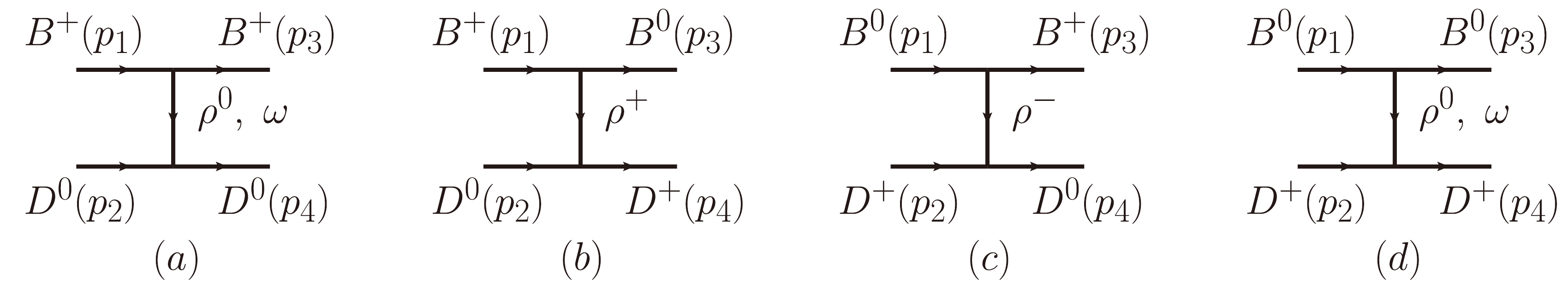
Figure 1. Vector exchange between the
$ D^{0}B^{+} $ and$ D^{+}B^{0} $ components (in brackets, the four momentum of each particle).$ V_{ij}=-\frac{1}{4f^2}\;C_{ij}\;(p_{1}+p_{2}) \cdot (p_{3}+p_{4});\quad f=93\ \text{MeV}, $

(1) with Cij the element of matrix C,
$ C_{ij}= \left(\begin{array}{*{20}{c}}{1 }&{1} \\{1} & {1} \end{array}\right), $

(2) and projected over S-wave
$ (p_{1}+p_{2})\cdot(p_{3}+p_{4})\to\frac{1}{2}\left[3s-2(m^2_{B}+m^2_{D})-\frac{(m_{B}^2-m_{D}^2)^2}{s}\right]. $

(3) The scattering matrix is then given by
$ T=[1-VG]^{-1}V, $

(4) where
$ G={{\rm{diag}}}(G_{1},G_{2}) $ , with$ G_{i} $ being the$ BD $ meson loop function regularized with a cutoff$ \begin{aligned}[b]G_i(\sqrt{s})=\;& \int_{|\vec q\,| < q_{\max}} \dfrac{{{\rm{d}}}^3 q}{(2\pi)^3} \; \dfrac{\omega_1(q)+\omega_2(q)}{2\,\omega_1(q)\, \omega_2(q)}\; \\&\times\dfrac{1}{s-[\omega_1(q)+\omega_2(q)]^2 + {\rm i} \varepsilon}, \end{aligned} $

(5) where
$ \omega_1(q)=\sqrt{\vec q^{\;2} +m_i^2} $ ,$ \omega_2(q)=\sqrt{\vec q^{\;2} +M_i^2} $ , and$ m_i, M_i $ are the masses of the D and B mesons in channel i. With the isospin states$ (B^{+}, B^{0}) $ ,$ (D^{+}, -D^{0}) $ , the$ I=0 $ combination is given by$ \left| {BD, I=0}\right\rangle=-\frac{1}{\sqrt{2}}\left| {B^+D^{0}+B^{0}D^+}\right\rangle, $

(6) with which we can obtain
$\langle B D, I=0|V| B D, I=0\rangle=\frac{1}{2}\left(V_{11}+V_{22}+2 V_{12}\right)=2 V_{11} ,$

(7) which is the result obtained in Ref. [39], with
$ V_{ij} $ given by Eqs. (1), (2), and (3). The$ I=1 $ combination is given by$\left|B D, I=1, I_3=0\right\rangle=-\frac{1}{\sqrt{2}}\left|B^+ D^0-B^0 D^+\right\rangle.$

(8) We reproduce the results of Ref. [39] using the cutoff regularization with an extra form factor (Eq. (27) from Ref. [39]) stemming from the S-wave projection of a vector meson exchange. However, practically identical results are obtained by ignoring this form factor and decreasing
$ q_{\text{max}} $ . To match the formalism of the correlation functions of Ref. [30], we ignore this form factor and take$ q_{\text{max}} $ of the order of$ 420 \; {\rm{MeV}} $ , as used in Ref. [45], to obtain the binding of the related$ T_{cc} $ state. -
We can evaluate the scattering length a,
$ r_{0} $ for the$ B^{+}D^{0} $ and$ B^{0}D^{+} $ channels by recalling the relationship between our T matrix and that used in quantum mechanics [64]$ T=-8\pi\sqrt{s}\;f^{QM}\simeq -8\pi\sqrt{s}\;\frac{1}{-\dfrac{1}{a}+\dfrac{1}{2}r_{0}k^2-{\rm i}k}, $

(9) with
$ k=\frac{\lambda^{1/2}(s,m_{1}^2,m_{2}^2)}{2\sqrt{s}}, $

(10) from which we easily find
$ -\frac{1}{a_{i}}=\left.\left(-8\pi\sqrt{s}\;T_{ii}^{-1}\right)\right|_{s_{{{\rm{th}}},i}}, $

(11) $ r_{0,i}=\left[\frac{2\sqrt{s}}{\mu_{i}}\frac{\partial}{\partial s}\left(-8\pi\sqrt{s}\;T_{ii}^{-1}+{\rm i}k_{i}\right)\right]_{s_{{{\rm{th}}},i}}, $

(12) where
$ \mu_{i} $ is the reduced mass in channel i, and$ s_{{{\rm{th}}},i} $ and$ k_{i} $ are the square of the threshold mass and the center of mass momenta of the mesons for channel i, respectively. -
We find that there is a pole, which is below the threshold of the two channels and hence corresponds to a bound state. The couplings are obtained from the T matrix in the vicinity of the pole,
$ T_{ij}=\frac{g_{i}\,g_{j}}{s-s_{p}}, $

(13) where
$ s_p $ is the square of the mass at the pole. Thus,$ g_{1}^2=\lim\limits_{s\to s_{p}}(s-s_{p})\;T_{11}, $

(14) $ g_{1}\,g_{j}=\lim\limits_{s\to s_{p}}(s-s_{p})\;T_{1j}, $

(15) which determine the relative sign of
$ g_2 $ with respect to$ g_1 $ . Once the couplings are evaluated, we calculate the molecular probabilities of the$ B^+ D^0 $ and$ B^0 D^+ $ channels, as in Refs. [64, 66, 67].$ {\cal{P}}_{i}=-g_{i}^2\left.\frac{\partial G_{i}}{\partial s}\right|_{s=s_{p}}. $

(16) Another magnitude of relevance is the wave function at the origin in coordinate space, given by [64]
$ \psi_{i}(r=0)=\left.g_{i}\,G_{i}\right|_{s_{{{\rm{th}}},i}}. $

(17) -
We follow the formalism of Ref. [30] and write the correlation functions for the two channels as
$ \begin{aligned}[b] C_{B^+D^0} (p_{D^0})=\;& 1+4\,\pi\, \theta(q_{\max}-p_{D^0})\, \int {\rm d} r \, r^2 S_{12}(r) \\ &\times \left\{\left|j_0(p_{D^0}\, r)+T_{B^+D^0, B^+D^0}(E)\; \tilde{G}^{(B^+D^0)}(r; E)\right|^2 \right. \\ &\;\left. + \left|T_{B^0D^+, B^+D^0}(E)\; \tilde{G}^{(B^0D^+)}(r; E) \right|^2 - j_0^2 (p_{D^0}\, r) \right\}, \end{aligned} $

(18) $ \begin{aligned}[b] C_{B^0D^+} (p_{D^+})=\;& 1+4\,\pi\, \theta(q_{\max}-p_{D^+})\, \int {\rm d}r \, r^2 S_{12}(r) \\ &\times \left\{\left|j_0(p_{D^+}\, r)+T_{B^0D^+, B^0D^+}(E)\; \tilde{G}^{(B^0D^+)}(r; E)\right|^2 \right. \\ &\;\left. + \left|T_{B^+D^0, B^0D^+}(E)\; \tilde{G}^{(B^+D^0)}(r; E) \right|^2 - j_0^2 (p_{D^+}\, r) \right\}, \end{aligned} $

(19) where
$ p_i $ is the momentum of the particles in the rest frame of the pair,$ p_i=\dfrac{\lambda^{1/2}(s, m_i^2, M_i^2)}{2\, \sqrt{s}}, $

(20) $ S_{12}(r) $ is the source function, parameterized as a Gaussian normalized to$ 1 $ ,$ S_{12}(r)= \dfrac{1}{(\sqrt{4\pi}\, R)^3} \; {\rm e}^{-(r^2/4R^2)}, $

(21) and the
$ \tilde{G}^{(i)}(r; E) $ function is defined as$ \tilde{G}^{(i)}(r; E)= \int \dfrac{{{\rm{d}}}^3 q}{(2\pi)^3} \; \dfrac{\omega_1(q)+\omega_2(q)}{2\,\omega_1(q)\, \omega_2(q)}\; \dfrac{j_0(q\, r)}{s-[\omega_1(q)+\omega_2(q)]^2 + {\rm i} \varepsilon}, $

(22) where
$ j_0(q\, r) $ is the spherical Bessel function, and$ E=\sqrt{s} = \sqrt{m_i^2 + \vec p_i^{\; 2}} + \sqrt{M_i^2 + \vec p_i^{\; 2}} $ . -
Here, we assume that the correlation functions have already been measured and attempt to extract the maximum information available using a general framework in which no model assumptions are made. To perform the test, we use the correlation function with the model described in the previous sections, assuming errors at the order of
$ \pm 0.02 $ , which are slightly larger than those obtained in current measurements of correlation functions.We begin by assuming that there is an interaction between the coupled channels, given by
$ V= \left(\begin{array}{*{20}{c}} {V_{11}} & {V_{12}} \\ {V_{12} }& {V_{22} } \end{array}\right), $

(23) where
$ V_{ij} $ are unknown potentials to be determined, and the T matrix is given by Eq. (4), using the G function of Eq. (5) with an unknown$ q_{\max} $ . We make no assumption on the isospin structure of a possible bound state but assume that the interaction is isospin symmetric, which implies, according to Eqs. (6), (7), and (8), that$\langle B D, \;I=0|V| B D, \;I=1\rangle=\frac{1}{2}\left(V_{11}-V_{22}\right)=0, $

(24) $ V_{22}=V_{11}. $

(25) In addition, to consider possible sources of interaction originating from channels neglected in our approach, we introduce several energy dependent terms, as discussed in Refs. [68, 69] and studied in [34–36]:
$ V_{11}=V_{11}'+\frac{\alpha}{m_{V}^2}(s-s_{{{\rm{th}}},1}), $

(26) $ V_{12}=V_{12}'+\frac{\beta}{m_{V}^2}(s-s_{{{\rm{th}}},1}), $

(27) where the factor
$ m^2_V $ (with$ m_V=800\; {\rm{MeV}} $ ) is introduced to make$ \alpha, \beta $ dimensionless. Then, we have$ 4 $ free parameters for the interaction, as well as$ q_{\max} $ and R, which is a total of$ 6 $ parameters to fit the two correlation functions. We must be aware that there are strong correlations between these parameters because the input used to obtain the correlation functions corresponds to an interaction at$ I=0 $ ; hence, what matters is the combination$ V_{11}+V_{12} $ . This means that the values we obtain for the parameters in fits to the pseudodata are not meaningful, and only the values of the observables obtained from them are significant. To manage with these correlations, we use the bootstrap or resampling method [70–72], generating random centroids of the data with a Gaussian distribution weight and performing a large number of fits to the data with the new centroids and same errors. After each fit, the values of the observables are evaluated, and the average and dispersion for each are calculated. -
Next, we use the model in Section II with a cutoff regularization of
$ q_{\max}=420\; {\rm{MeV}} $ , as in the study of the$ T_{cc} $ state in Ref. [45]. We obtain a pole at$ \sqrt{s}=7110.41 $ MeV and the couplings given in Table 1. Similarly, the probabilities obtained and the wave functions at the origin are given in Table 2, and the scattering length and effective range are shown in Table 3. As shown, the probability obtained for the sum of the two$ B^+D^0, B^0D^+ $ channels is of the order of 96%. The small deviation from unity is due to the energy dependence of the original potential of Eqs. (1) and (3). We also observe that while$ a_1, r_{0,1} $ are real,$ a_2, r_{0, 2} $ are complex because the$ B^+D^0 $ channel is open at the threshold of the$ B^0 D^+ $ channel. The couplings are very similar, and so are the wave functions at the origin, indicating an$ I=0 $ state, according to Eq. (6). The results for the correlation functions of the two channels are shown in Fig. 2, calculated with$ R=1\, {\rm{fm}} $ .$ \sqrt{s_p} $ 

$ g_1 $ 

$ g_2 $ 

$(7110.41+0\,{\rm i})$ 

$ 31636.8 $ 

$ 31631.0 $ 

Table 1. Pole position and couplings with
$ q_{\max}=420\; {{\rm{MeV}}} $ . [in units of MeV]$ {\cal{P}}_1 $ 

$ {\cal{P}}_2 $ 

$ \psi_1(r=0) $ 

$ \psi_2(r=0) $ 

$ 0.52 $ 

$ 0.44 $ 

$ -14.75 $ 

$ -13.61 $ 

Table 2. Probability
$ {\cal{P}}_i $ and wave function at the origin$ \psi_i(r=0) $ for channel i.$ a_{1} $ 

$ a_{2} $ 

$ r_1 $ 

$ r_2 $ 

$ 0.71 $ 

$0.50-0.16\,{\rm i}$ 

$ -0.61 $ 

$1.22-1.77\,{\rm i}$ 

Table 3. Scattering length
$ a_i $ and effective range$ r_{i} $ for channel i. [in units of fm]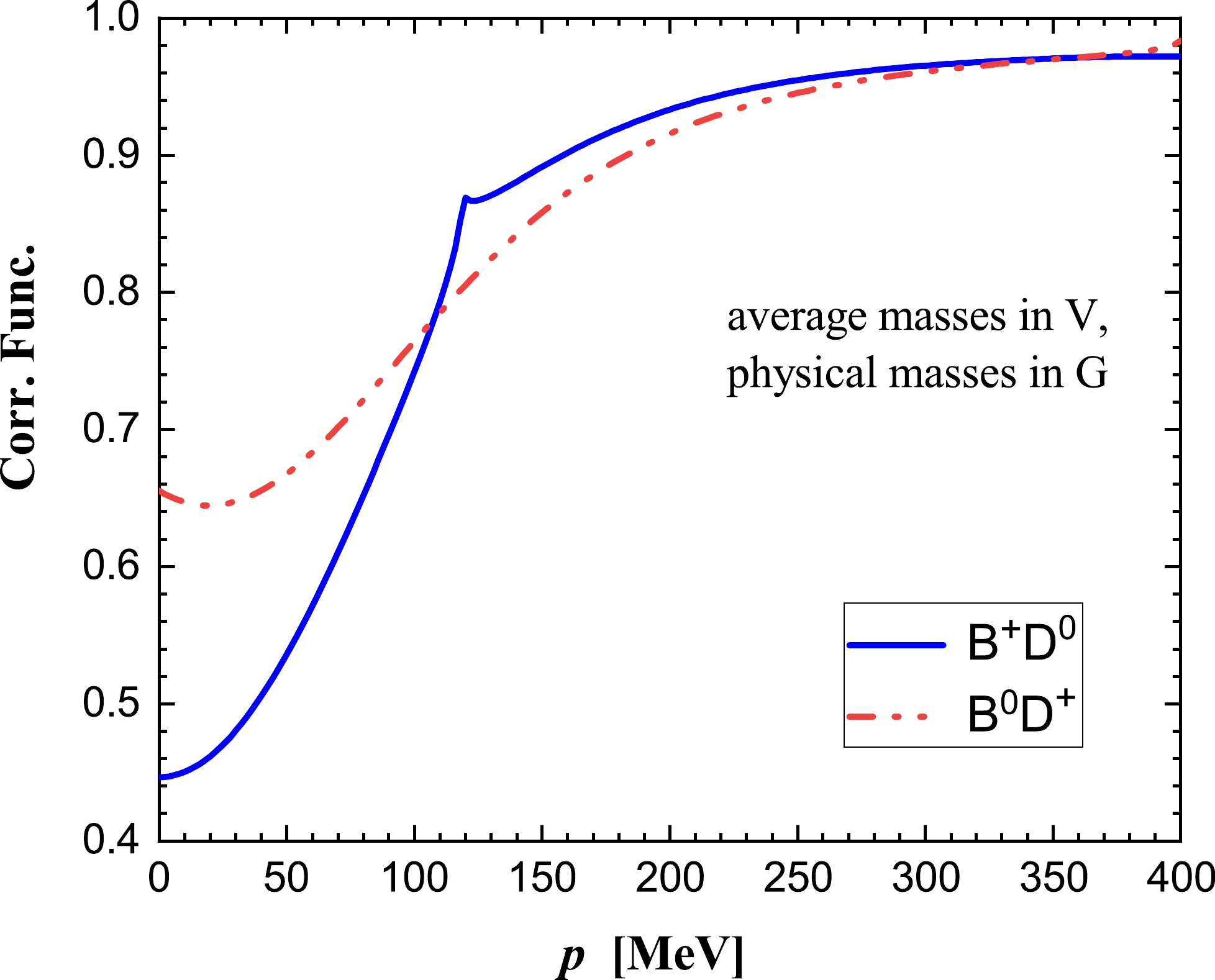
Figure 2. (color online) Correlation functions for the
$ B^+D^0 $ and$ B^0D^+ $ channels.Next, we discuss the results obtained from the resampling method fits to the data. The data with the assumed errors are shown in Fig. 3. A warning should be given: as discussed in detail in Ref. [36], the sign of
$ V_{12} $ is undefined in the present procedure; however, we rely on arguments of heavy quark flavor symmetry to choose solutions with$ V_{11} $ and$ V_{12} $ of the same sign.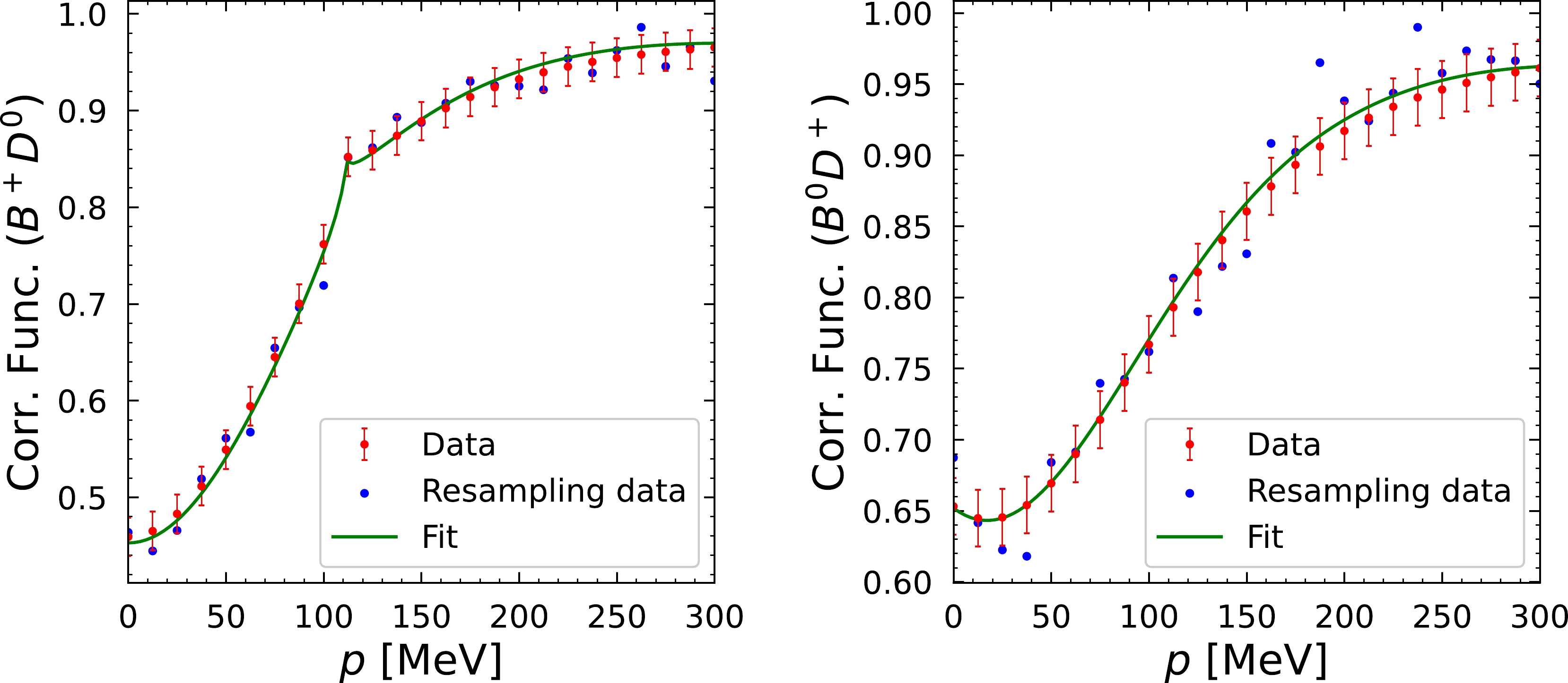
Figure 3. (color online) Correlation functions for the
$ B^+D^0 $ (left) and$ B^0D^+ $ (right) channels, with 26 points in each curve with an error of$ \pm 0.02 $ . The centroids of the red data follow the theoretical curve. In blue, we plot the centroids obtained in one of the resampling runs, with a random Gaussian generation of the centroids of each point.In Table 4, we show the average values and dispersion of the parameters obtained. As we discussed above, they are not significative owing to the existing correlations. One indication of these correlations is the relatively large parameter errors. Nevertheless, the important aspect is the value of the observables. These can be found in Tables 5, 6, and 7.
$ V'_{11} $ 

$ V'_{12} $ 

α β $q_{\max} /{\rm{MeV} }$ 

$R /{\rm{fm} }$ 

$ -1537.54\pm 918.93 $ 

$ -1512.32\pm 913.55 $ 

$ -31.89\pm 10.00 $ 

$ -165.16\pm 133.31 $ 

$ 407.9\pm 60.8 $ 

$ 1.01 \pm 0.04 $ 

Table 4. Values obtained for the parameters
$ V'_{11}, V'_{12} $ ,$ \alpha, \beta $ ,$ q_{\max} $ , and R.$ \sqrt{s_p} $ 

$ g_1 $ 

$ g_2 $ 

$ 7107.84\pm 17.79 $ 

$ 34623.08\pm 14300.15 $ 

$ 34506.64 \pm 14304.57 $ 

Table 5. Average values and dispersion of the pole position and couplings. [in units of MeV]
$ {\cal{P}}_1 $ 

$ {\cal{P}}_2 $ 

$ \psi_1(r=0) $ 

$ \psi_2(r=0) $ 

$ 0.49 \pm 0.03 $ 

$ 0.42 \pm 0.03 $ 

$ -13.61\pm 2.65 $ 

$ -12.61\pm 2.423 $ 

Table 6. Average value and dispersion of the probability
$ {\cal{P}}_i $ and wave function at the origin$ \psi_i(r=0) $ for channel i.$ a_{1} $ 

$ a_{2} $ 

$ r_1 $ 

$ r_2 $ 

$ 0.72\pm 0.03 $ 

$ (0.51\pm 0.02)-$ 

$(0.17 \pm 0.01)\,{\rm i}$ 

$ -0.61\pm 0.19 $ 

$ (1.41\pm 0.28)- $ 

$(1.65\pm 0.07)\,{\rm i}$ 

Table 7. Average value and dispersion of the scattering length
$ a_i $ and effective range$ r_{i} $ for channel i. [in units of fm]In Table 5, we show the value of the energy at which the bound state is found, together with the values of the couplings. As shown, a bound state is found around
$ 7108\; {\rm{MeV}} $ , compatible with the bound state obtained with the original model within uncertainties. Interestingly, the error obtained is of the order of$ 18\; {\rm{MeV}} $ . This is not a small error for a binding energy of$ 39\; {\rm{MeV}} $ ; however, this is what can be achieved with the assumed precision of the correlation data. More positively, using the data of the correlations at the$ BD $ threshold, we are still able to predict that there is a bound state with an approximately$ 40\; {\rm{MeV}} $ binding.The couplings
$ g_1, g_2 $ obtained are also compatible with the original ones, and the errors are also not small. Yet, the approximately equal values of the couplings suggest that we are dealing with an$ I=0 $ state.It is interesting to analyze our obtained probabilities of the states, which are shown in Table 6. We again obtain numbers for the probabilities of the two channels compatible with those obtained from the original model, but once again, it is the precision by which they can be obtained that is important. The uncertainties are very small, that is, of the order of 6%. This may be surprising in view of the formula used to obtain
$ {\cal{P}}_i $ (Eq. (16)), which is proportional to$ g_i^2 $ , and$ g_i $ has large errors according to Table 5. If$ g_i^2 $ is bigger in a fit because the state is more bound,${\partial G_{i}}/{\partial s}$ also decreases in strength and the product becomes more stable. This is an interesting and fortunate result of our analysis, which allows us to conclude that the application of the inverse method from the femtoscopic correlation functions would allow us to determine the nature of the bound state obtained with a high accuracy.As shown in Table 7, it is also rewarding to find that we can determine the scattering lengths with good precision and the effective ranges with smaller precision but significant values.
We should also stress that the inverse method allows us to obtain the size of the source function with a relative accuracy of approximately 4% (see Table 4).
-
We address the problem of evaluating the correlation functions for the
$ BD $ system using inputs extracted from a successful study of the$ T_{cc}(3875) $ state. We take two channels,$ B^0 D^+ $ and$ B^+ D^0 $ , the small mass differences between which induce visible differences in the correlation functions. The system also develops a bound state of approximately 40 MeV. Once this is achieved, we address the inverse problem of obtaining the observables associated with this system, starting from the correlation functions, assuming errors as in current measurements. Although we obtain results compatible with those obtained from the original model, an important new result is the uncertainty by which we can obtain the observables of the system. We obtain the size of the source with a precision of approximately 4%. We also determine that there is a bound state using the data of the correlation functions above the threshold of the channels, although with an uncertainty of approximately 50% of the binding energy. However, remarkably, we can determine the molecular nature of the obtained state with a good precision of approximately 6%. The scattering lengths of the two channels are obtained with good precision and significant values, and the effective ranges are also obtained but with smaller precision. All these results indicate that the measurement of these correlation functions in the future will allow us to obtain valuable information on the$ BD $ interaction and the bound states associated with this interaction. This study could serve as motivation to conduct such measurements in the future.
Correlation function and the inverse problem in the BD interaction
- Received Date: 2024-02-07
- Available Online: 2024-05-15
Abstract: We study the correlation functions of the


 DownLoad: