


 Abstract
 HTML
HTML Reference
 Related
 PDF
PDF


-
The top quark is the heaviest elementary particle in the Standard Model (SM), and its mass is one of the most important input parameters of the SM. The largest mass among quarks, or equivalently the strongest Yukawa coupling, implies that the top quark plays a crucial role in governing the stability of the electroweak vacuum. Determining the top-quark mass accurately is helpful for testing the precision of the SM, assessing whether the vacuum is in stable or meta-stable state, and searching for new physics beyond the SM. Direct measurements of the top-quark mass exhibit high precision in proton-proton (
$ pp $ ) collisions at the LHC [1–8]; these measurements rely on the reconstruction of the top quark decay products and multipurpose Monte Carlo (MC) event generators. Other measurements were also reported in Refs. [9–17]. In the theoretical side, many studies aimed to relate the top-quark mass to its on-shell (OS) scheme mass, c.f. Refs. [18–25]. A$ 0.5\sim 1 $ GeV difference between the top-quark MC mass ($ M_t^{{\rm{MC}}} $ ) and top-quark OS mass ($ M_t^{{\rm{OS}}} $ ) has been reported [26–32].The top-quark OS mass has been investigated in detail in Refs. [33–52]. This mass can be related to the modified minimal subtraction (
$ \overline{{\rm{MS}}} $ ) scheme running mass by using the perturbative relations between the top-quark bare mass ($ m_{t,0} $ ) and renormalized mass in the OS- or$ \overline{{\rm{MS}}} $ - scheme, e.g.,$ m_{t,0}=Z^{{\rm{OS}}}_{m}M_t^{{\rm{OS}}} $ and$ m_{t,0}=Z^{\overline{{\rm{MS}}}}_{m}{{\overline{m}}}_t(\mu_r) $ . In these expressions,$ Z^{{\rm{OS}}}_{m} $ and$ Z^{\overline{{\rm{MS}}}}_{m} $ are quark mass renormalization constants in the OS- and$ \overline{{\rm{MS}}} $ - schemes, respectively. In perturbative Quantum Chromodynamics (pQCD) theory, the relation between the OS mass and$ \overline{{\rm{MS}}} $ mass has been calculated up to four-loop level [53–65]. This allows for determining the OS mass with the help of experimental results for the$ \overline{{\rm{MS}}} $ mass. In the determination process, the key issue is to set the exact values of the strong coupling constant ($ \alpha_s $ ) and$ \overline{{\rm{MS}}} $ mass (e.g.,$ {{\overline{m}}}_q $ ,$ q=c,b,t $ denote the charm, bottom, and top quarks, respectively). The scale running behavior of$ \alpha_s $ and$ {{\overline{m}}}_q $ is governed by general renormalization group equations (RGEs) involving both the β function and quark mass anomalous dimension$ \gamma_m $ :$ \frac{{\rm d} a_s(\mu_r)} {{\rm d}\ln\mu^2_r}= \beta(a_s)=-\sum\limits_{i=0}^\infty \beta_i a^{i+2}_s(\mu_r), $

(1) $ \frac{{\rm d}{{\overline{m}}}_q(\mu_r)}{{\rm d}\ln{\mu_r^2}} = {{\overline{m}}}_q(\mu_r) \gamma_m(a_s)=-{{\overline{m}}}_q(\mu_r) \sum\limits_{i=0}^\infty \gamma_i a^{i+1}_s(\mu_r), $

(2) where
$ a_s(\mu_r)=\alpha_s(\mu_r)/(4\pi) $ . The$ \{\beta_i\} $ - and$ \{\gamma_i\} $ -functions have been calculated up to five-loop level in the$ \overline{{\rm{MS}}} $ -scheme [66–74], e.g.,$ \beta_0=11-{2}n_f/{3} $ and$ \gamma_0=4 $ , where$ n_f $ is the number of active flavors. Using reference points such as$ \alpha_s(M_Z)=0.1179\pm 0.0009 $ and$ {{\overline{m}}}_t({{\overline{m}}}_t)=162.5^{+2.1}_{-1.5} $ GeV, reported by the Particle Data Group [75], their values can be obtained at any scale.Because of renormalization group invariance (RGI), the physical observable is independent of any choices of renormalization scheme and scale. However, for a fixed-order pQCD prediction, the mismatching of
$ \alpha_s $ and the pQCD coefficients at each order leads to the well-known renormalization scheme-and-scale ambiguities. To eliminate such artificially introduced renormalization scheme-and-scale ambiguities, the principle of maximum conformality (PMC) was proposed [76–79]. This principle sets the underlying procedure for the well-known Brodsky-Lepage-Mackenzie (BLM) method [80] as well as a rule for generalizing the BLM procedure up to all orders. A short review of the development of the PMC from the BLM method can be found in Ref. [81]. All the features previously observed in the studies on the BLM method are also adaptable to the PMC with or without proper transformations, e.g., only the RG-involved$ n_f $ -terms in the pQCD series should be treated as non-conformal terms and be adopted for setting the correct magnitude of$ \alpha_s $ . The PMC thus provides a rigorous scale-setting approach for obtaining unambiguous fixed-order pQCD predictions consistent with the principles of the renormalization group1 . Moreover, its predictions satisfy all the requirements for renormalization group invariance [87, 88]. A complete discussion about the PMC can be found in review articles [89–91].To date, the PMC method has been successfully applied to many high-energy processes, c.f. Refs. [92–98], aiming to determine the correct magnitude of the strong running coupling
$ \alpha_s $ of the pQCD series by using the procedures suggested in Refs. [99, 100]. However, there are also many other advances related to both the running coupling$ \alpha_s $ and quark$ \overline{{\rm{MS}}} $ running mass$ \overline{m}_q $ . If the pQCD series contains both the$ n_f $ -terms related to the renormalization of$ \alpha_s $ and the$ n_f $ -terms related to the renormalization of$ {{\overline{m}}}_q $ , some extra treatments must be applied before using the formulas listed in Refs. [99, 100]; those formulas are based on the assumption that both the conformal and non-conformal terms have been correctly distributed2 . To achieve a correct PMC prediction, the degeneracy relations among different orders, which jointly constitute a general property of the QCD theory [103], should be applied correctly. In this paper, we derive new degeneracy relations with the help of the RGEs involving both the β-function and quark mass anomalous dimension$ \gamma_m $ -function, which lead to improved PMC scale-setting procedures. Such procedures are then applied for determining the top-quark OS mass by simultaneously determining the correct magnitudes of$ \alpha_s $ and quark$ \overline{{\rm{MS}}} $ running mass$ {{\overline{m}}}_q $ of the perturbative series with the help of RGEs for either the running coupling$ \alpha_s $ or running mass.The rest of this paper is organized as follows. In Sec. II, we describe the special degeneracy relations of the non-conformal terms in the perturbative coefficients by using the
$ {{\cal{R}}}_\delta $ -scheme. Then, we elaborate on the improved procedures of the PMC scale-setting approach under the running mass scheme. We apply these procedures in Sec. III to determine the top-quark OS mass$ M_t $ via its perturbative relation to the$ \overline{{\rm{MS}}} $ mass. Section IV presents a summary. -
The
$ {{\cal{R}}}_\delta $ -scheme represents the$ {{\rm{MS}}} $ -type renormalization scheme with a subtraction term$ \ln(4\pi)-\gamma_{E}-\delta $ , where δ is an arbitrary finite number [99] satisfying that$ {{\cal{R}}}_{\delta=0}=\overline{{\rm{MS}}} $ . As an extension of Ref. [99], we consider the pQCD prediction$ \rho(Q^2) $ including the$ \overline{{\rm{MS}}} $ running mass. In the reference scheme$ {{\cal{R}}}_0 $ , this prediction can be expressed as follows:$ \rho_0(Q^2)=r_0 {{\overline{m}}}_q^n(\mu_r)\bigg[1+\sum\limits_{k=1}^\infty r_{k}(\mu_r^2/Q^2)a_s^k(\mu_r)\bigg], $

(3) where
$ \rho_0 $ denotes the pQCD prediction ρ in the$ {{\cal{R}}}_0 $ scheme, Q represents a physical scale of the measured observable3 ,$ {{\overline{m}}}_q $ is the quark$ \overline{{\rm{MS}}} $ running mass, n is the power of$ {{\overline{m}}}_q $ associated with the tree-level term, and$ r_0 $ is a global factor. For simplicity, we assume that$ r_0 $ does not have$ a_s $ . The pQCD series is independent of the choice of renormalization scale$ \mu_r $ , provided that it has been calculated up to all orders. However, it is not feasible to achieve this goal owing to the difficulty of high-order calculations. Generally, the pQCD series becomes a renormalization scale that depends on the scheme at any finite order; this dependence can be exposed by using the$ {{\cal{R}}}_\delta $ -scheme. One can derive the general expression for ρ in$ {{\cal{R}}}_\delta $ by using the scale displacements in any$ {{\cal{R}}}_\delta $ -scheme:$ a_s(\mu_r) = a_s(\mu_\delta) + \sum\limits_{n=1}^\infty \frac{1}{n!} { \frac{{{\rm{d}}}^n a_s(\mu_r)}{({{\rm{d}}} \ln \mu_r^2)^n}{\bigg |}_{\mu_r=\mu_\delta}(-\delta)^n}, $

(4) $ {{\overline{m}}}_q(\mu_r) = {{\overline{m}}}_q(\mu_\delta)+\sum\limits_{n=1}^\infty\frac{1}{n!}\frac{d^n{{\overline{m}}}_q(\mu_r)}{(d\ln{\mu_r^2})^n}{\bigg |}_{\mu_r=\mu_\delta}(-\delta)^n, $

(5) where
$ \delta=-\ln{(\mu_r^2/\mu_\delta^2)} $ . It is useful to derive the general displacement relations as expansions up to fixed order, as shown in Appendix A.Inserting these scale displacements into Eq. (3), one can obtain the expression of
$ \rho_\delta $ for an arbitrary δ in any$ {{\cal{R}}}_\delta $ -scheme:$ \begin{aligned}[b] \rho_\delta(Q^2)=\;& r_0 {{\overline{m}}}_q^n(\mu_{\delta})\{1+(r_1+n \gamma_0 \delta)a_s(\mu_{\delta}) \\ &+[r_2+\beta_0r_1\delta+n(\gamma_1+\gamma_0r_1)\delta+\frac{n}{2}\beta_0\gamma_0\delta^2\\ &+\frac{n^2}{2}\gamma_0^2\delta^2]a^2_s(\mu_{\delta})+{\rm{O}}[a^3_s(\mu_{\delta})]\}, \end{aligned} $

(6) where
$ \rho_\delta $ denotes the pQCD prediction ρ in the$ {{\cal{R}}}_\delta $ scheme and$ \mu_{\delta}^2=\mu_r^2 e^\delta $ . A useful expression of$ \rho_\delta $ up to$ a_s^4 $ -order is provided in Appendix B. It is easy to return to$ \rho_0 $ by setting$ \delta=0 $ . A further description of the$ {{\cal{R}}}_\delta $ -scheme can be found in Sec. II of Ref. [99].The renormalization group invariance requires that the perturbative series up to all orders for a physical observable be independent of the theoretical convention:
$ \begin{aligned}[b]\frac{{\rm d} \rho_{\delta}}{{\rm d} \delta}&=\frac{\partial \rho_{\delta}}{\partial \delta}+\beta(a_s)\frac{\partial \rho_{\delta}}{\partial a_s}+{{\overline{m}}}_q \gamma_m(a_s)\frac{\partial \rho_{\delta}}{\partial {{\overline{m}}}_q}.\\& = 0. \end{aligned} $

(7) Thus, we can obtain
$ \frac{\partial \rho_{\delta}}{\partial \delta}=-\beta(a_s)\frac{\partial \rho_{\delta}}{\partial a_s}-{{\overline{m}}}_q \gamma_m(a_s)\frac{\partial \rho_{\delta}}{\partial {{\overline{m}}}_q}. $

(8) Therefore, by absorbing all
$ \{\beta_i\} $ and$ \{\gamma_i\} $ dependences into the running coupling constant and quark running mass in Eq. (6), one can obtain a scheme-invariant prediction given that the δ-dependence is vanished. Therefore, the coefficients of the resultant series will be equal to those of the conformal (or scale-invariant) theory, that is,$ \partial \rho_\delta /\partial \delta = 0 $ .The expression in Eq. (6) also exposes the pattern of
$ \{\beta_i\} $ -terms and$ \{\gamma_i\} $ -terms in the coefficients at each order. Given that there is nothing special about any particular value of δ, it is possible to infer some degenerate relations between certain coefficients of the$ \{\beta_i, \gamma_i\} $ -terms from the expression$ \rho_\delta $ . That is, the coefficients of$ \beta_0 a_s^2 $ and$ n\gamma_0 a_s^2 $ can be set equal, given that their coefficients are both$ r_1\delta $ . Therefore, for any scheme, the expression for ρ can be transformed into a similar form to that of$ \rho_\delta $ :$ \begin{aligned}[b] \rho(Q^2)=\;& r_0 {{\overline{m}}}_q^n(\mu_r)\bigg\{1+\left({\hat r}_{1,0}+n\gamma_0\ln\frac{\mu_r^2}{Q^2}\right) a_s(\mu_r) \\ &+\bigg[{\hat r}_{2,0}+\beta_0{\hat r}_{2,1}+n\gamma_0{\hat r}_{2,1} \\ &+\left(\beta_0{\hat r}_{1,0}+n\gamma_1+n\gamma_0{\hat r}_{1,0}\right)\ln\frac{\mu_r^2}{Q^2} \\ &+\frac{1}{2}\left(n\beta_0\gamma_0+n^2\gamma_0^2\right)\ln^2\frac{\mu_r^2}{Q^2}\bigg] a^2_s(\mu_r) \\ &+ {\rm{O}}[a^3_s(\mu_r)]\bigg\}, \end{aligned} $

(9) where
$ {\hat r}_{i,j} $ are coefficients that do not depend on$ \mu_r $ ,$ {\hat r}_{i,0} $ are conformal coefficients, and the$ \{\beta_i, \gamma_i\} $ -terms are non-conformal terms. A useful expression up to$ a_s^4 $ -order is provided in Appendix C. It is easy to find the relationships between the coefficients$ r_{k}(\mu_r^2/Q^2) $ and$ {\hat r}_{i,j} $ :$ r_{1}(\mu_r^2/Q^2)= {\hat r}_{1,0}+n\gamma_0\ln\frac{\mu_r^2}{Q^2}, $

(10) $ \begin{aligned}[b] r_{2}(\mu_r^2/Q^2)=\;& {\hat r}_{2,0}+\beta_0{\hat r}_{2,1}+n\gamma_0{\hat r}_{2,1} \\ &+ (\beta_0{\hat r}_{1,0}+n\gamma_1+n\gamma_0{\hat r}_{1,0})\ln\frac{\mu_r^2}{Q^2} \\ &+ \frac{1}{2}(n\beta_0\gamma_0+n^2\gamma_0^2)\ln^2\frac{\mu_r^2}{Q^2}, \end{aligned} $

(11) The relationships between the coefficients
$r_{k}(\mu_r^2/Q^2) (k=3,4)$ and$ {\hat r}_{i,j} $ are provided in Appendix D. These relationships lead to systematic procedures to determine the coefficients$ {\hat r}_{i,j} $ . In some cases, the coefficients$ r_{k}(\mu_r^2/Q^2) $ in Eq. (3) are computed numerically, and the$ \{\beta_i, \gamma_i\} $ dependence is not known explicitly. However, it is straightforward to obtain the dependence on the number of quark flavors$ n_f $ , because$ n_f $ enters analytically in any loop diagram computation. To apply the PMC scale-setting approach, one should put the pQCD expression into the form of Eq. (9). Owing to the special degeneracy relations in the coefficients of$ \{\beta_i, \gamma_i\} $ -terms, the$ n_f $ series can be matched to the$ {\hat r}_{i,j} $ coefficients in a unique manner. The$ k_{{\rm{th}}} $ -order coefficient in pQCD has an expansion in$ n_f $ that reads$ r_{k}(\mu_r^2/Q^2)=c_{k,0}+c_{k,1}n_f+...+c_{k,k-1}n_f^{k-1}, $

(12) where the coefficients
$ c_{k,l} $ are obtained from the pQCD calculation and are a function of$ \mu_r $ and Q. Then, the coefficients$ {\hat r}_{i,j} $ in Eq. (9) can be determined by using their relationship with$ r_{k}(\mu_r^2/Q^2) $ and the known coefficients$ c_{k,l} $ . The steps are detailed in Appendix E. In the next section, we will show improved PMC formulas under the running mass scheme. -
Adopting the PMC single-scale approach [100], the overall effective running coupling
$ a_s(Q_*) $ and effective running mass$ {{\overline{m}}}_q(Q_*) $ can be determined by absorbing all the non-conformal terms. Eq. (9) transforms into the following conformal series:$ \begin{aligned}[b] \rho(Q^2)=\;& r_0 {{\overline{m}}}_q^n(Q_*)\big\{1+{\hat r}_{1,0}a_s(Q_*) + {\hat r}_{2,0}a_s^2(Q_*) \\ &+ {\hat r}_{3,0}a_s^3(Q_*)+{\hat r}_{4,0}a_s^4(Q_*)+{\rm{O}}[a^5_s(Q_*)]\big\}, \end{aligned} $

(13) where
$ Q_* $ is the PMC scale. More explicitly, by using the scale displacement relations to shift the scale$ \mu_r $ to$ Q_* $ in Eq. (9), the PMC scale$ Q_* $ can be determined by requiring that all non-conformal terms (NonConf.) vanish:$ \begin{aligned}[b] \rho(Q^2)_{{\rm{NonConf}}.}=\;& r_0 {{\overline{m}}}_q^n(Q_*)\{r_{\rm 1, NonConf.}(Q_*) a_s(Q_*) \\ &+ r_{\rm 2, NonConf.}(Q_*) a^2_s(Q_*) \\ &+ r_{\rm 3, NonConf.}(Q_*) a^3_s(Q_*) \\ &+ r_{\rm 4, NonConf.}(Q_*) a^4_s(Q_*)+{{\cal{O}}}[a^5_s(Q_*)]\} \\ =\;& 0, \end{aligned} $

(14) where
$ r_{\rm 1, NonConf.}(Q_*) = n\gamma_0\ln\frac{Q_*^2}{Q^2}, $

(15) $ \begin{aligned}[b] r_{\rm 2, NonConf.}(Q_*)=\;& \beta_0{\hat r}_{2,1}+n\gamma_0{\hat r}_{2,1} \\ &+(\beta_0{\hat r}_{1,0}+n\gamma_1+n\gamma_0{\hat r}_{1,0})\ln\frac{Q_*^2}{Q^2} \\ &+\frac{1}{2}(n\beta_0\gamma_0+n^2\gamma_0^2)\ln^2\frac{Q_*^2}{Q^2}, \end{aligned} $

(16) where the higher-order coefficients
$r_{i,\rm NonConf.}(i=3,4)$ are provided in Appendix F.Owing to its perturbative nature, the solution of
$ \ln(Q^2_*/Q^2) $ can be expanded as a power series over$ a_s(Q_*) $ :$ \ln\frac{Q^2_*}{Q^2}=\sum\limits_{i=0}^{n} S_{i}a^i_s(Q_*), $

(17) where
$ S_i $ are perturbative coefficients that can be derived by solving Eq. (14). For$ n\neq0 $ , the first three coefficients$ S_i(i=0,1,2) $ are$ S_0 = 0, $

(18) $ S_1 = -\frac{(\beta_0+n\gamma_0){\hat r}_{2,1}}{n\gamma_0}, $

(19) $ \begin{aligned}[b] S_2=\;& {\hat r}_{1,0}{\hat r}_{2,1}-{\hat r}_{3,1}-\frac{n\gamma_0{\hat r}_{3,2}}{2}-\frac{\beta_1{\hat r}_{2,1}}{n\gamma_0}\\ &+\beta_0\left(\frac{\gamma_1{\hat r}_{2,1}}{n\gamma_0^2}+\frac{2{\hat r}_{1,0}{\hat r}_{2,1}-2{\hat r}_{3,1}}{n\gamma_0}-\frac{3{\hat r}_{3,2}}{2}\right)\\ &+\beta_0^2\left(\frac{{\hat r}_{1,0}{\hat r}_{2,1}}{n^2\gamma_0^2}-\frac{{\hat r}_{3,2}}{n\gamma_0}\right), \end{aligned} $

(20) and
$ S_3 $ is provided in Appendix G. Following this idea, the PMC scale$ Q_* $ can be fixed at any order; the correct magnitudes of the quark running mass$ {{\overline{m}}}_q $ and running coupling constant$ a_s $ are determined simultaneously. Matching the$ \mu_r $ -independent conformal coefficients$ {\hat r}_{i,0} $ , the resultant PMC series will be free of conventional renormalization scale ambiguity. In the following section, we apply these formulas to determine the top-quark OS mass$ M_t $ via its perturbative relation to the$ \overline{{\rm{MS}}} $ mass. -
For numerical calculations, we adopted
$\alpha_s(M_Z)= 0.1179\pm 0.0009$ and$ {{\overline{m}}}_t({{\overline{m}}}_t)=162.5^{+2.1}_{-1.5} $ GeV [75]. The running of the strong coupling$ \alpha_s(\mu_r) $ was evaluated using the RunDec program [104]. -
The relation between the
$ \overline{{\rm{MS}}} $ quark mass and OS quark mass can be expressed as$ \frac{{{\overline{m}}}_t(\mu_r)}{M_t}=\frac{Z_m^{{\rm{OS}}}}{Z_m^{\overline{{\rm{MS}}}}}=\sum\limits_{n\geq0}a^n_s(\mu_r) z^{(n)}_m(\mu_r), $

(21) where
$ z^{(0)}_m(\mu_r)=1 $ and$ z^{(n)}_m(\mu_r) $ is a function of$ \ln(\mu_r^2/M_t^2) $ . As an expansion of a previous study [95], we focus on the inverted relation with respect to Eq. (21),$ \frac{M_t}{{{\overline{m}}}_t(\mu_r)}=\frac{Z_m^{\overline{{\rm{MS}}}}}{Z_m^{{\rm{OS}}}}=\sum\limits_{n\geq0}a^n_s(\mu_r) c^{(n)}_m(\mu_r), $

(22) where
$ c^{(0)}_m(\mu_r)=1 $ and$ c^{(n)}_m(\mu_r) $ is a function of$ \ln(\mu_r^2/{{\overline{m}}}_t^2(\mu_r)) $ . Then, we can determine the top-quark OS mass using the following relationship:$ \begin{aligned}[b] M_t=\;& {{\overline{m}}}_t(\mu_r)\{1+r_1(\mu_r)a_s(\mu_r) + r_2(\mu_r)a_s^2(\mu_r)\\ &+ r_3(\mu_r)a_s^3(\mu_r)+ r_4(\mu_r)a_s^4(\mu_r)+{\rm{O}}[a^5_s(\mu_r)]\}, \end{aligned} $

(23) where the perturbative coefficients
$ r_i(\mu_r)(i=1,2,3,4) $ were reported in Refs. [61, 62] and$ r_i(\mu_r) $ are functions of$ \ln (\mu_r^2/{{\overline{m}}}_t^2(\mu_r)) $ . The$ \mu_r $ dependence of the top-quark$ \overline{{\rm{MS}}} $ running mass$ {{\overline{m}}}_t(\mu_r) $ is governed by the quark mass anomalous dimension$ \gamma_m $ , which has been calculated up to$ {{\cal{O}}}(\alpha_s^5) $ [71, 72]. Thus, the top-quark$ \overline{{\rm{MS}}} $ running mass$ {{\overline{m}}}_t(\mu_r) $ can be determined by the following equation [72]:$ {{\overline{m}}}_t(\mu_r)={{\overline{m}}}_t({{\overline{m}}}_t)\frac{c_t[\alpha_s(\mu_r)/\pi]}{c_t[\alpha_s({{\overline{m}}}_t)/\pi]}, $

(24) where
$c_t[x]=x^{4/7}(1+1.19796x+ 1.79348x^2- 0.683433x^3 -3.53562x^4)$ .By setting all input parameters to their central values, the top-quark OS mass
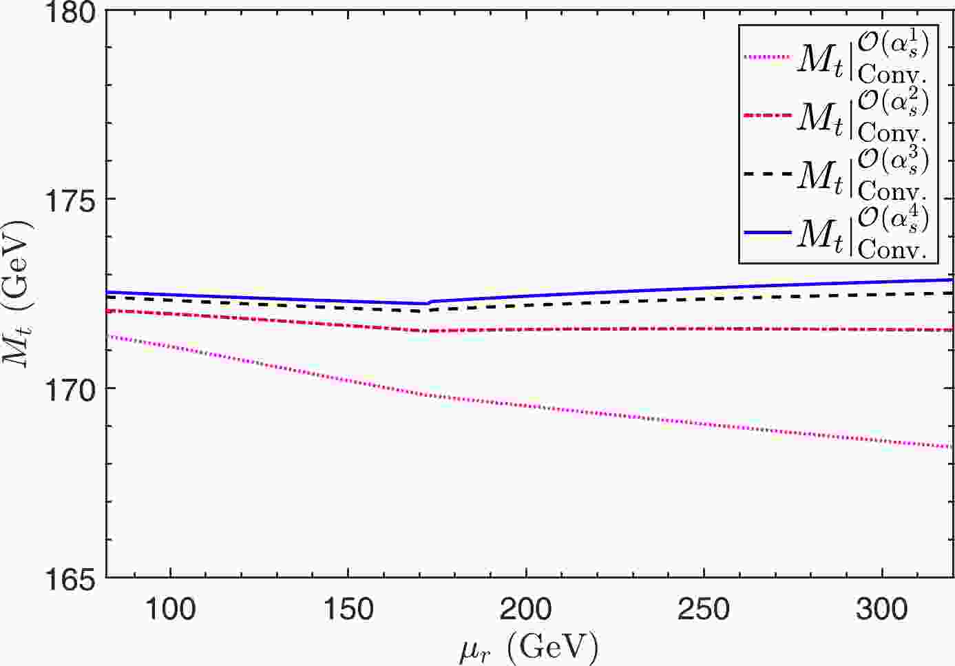
$ M_t $ under the conventional scale-setting approach can be represented as depicted in Fig. 1. In particular, Fig. 1 shows that, in agreement with conventional wisdom, the renormalization scale dependence of conventional series becomes smaller when more loop terms have been included. Numerically, we have$ M_t|_{{\rm{Conv}}.}^{{\rm{O}}(\alpha_s^4)} =[172.23,172.88] $ for$ \mu_r \in [{{\overline{m}}}_t({{\overline{m}}}_t)/2, 2{{\overline{m}}}_t({{\overline{m}}}_t)] $ ; e.g., the net scale uncertainty becomes ~0.4% for a$ \alpha_s^4 $ -order correction. This small net scale dependence for the prediction up to$ a_s^4 $ -order is due to the well convergent behavior of the perturbative series. The relative magnitudes among different orders change significantly for different choices of$ \mu_r $ ; for example, the relative magnitudes of the leading-order-terms (LO): next-to-leading-order-terms (NLO): next-to-next-to-leading-order-terms (N2LO): next-to-next-to-next-to-leading-order-terms (N3LO): next-to-next-to-next-to-next-to-leading-order-terms (N4LO)$ \simeq $ 1: 4.60%: 0.98%: 0.30%: 0.12% for$\mu_r= {{\overline{m}}}_t({{\overline{m}}}_t)$ , which represents a proper perturbative nature. More specifically,$ M_t $ up to N4LO-level has the following perturbative behavior: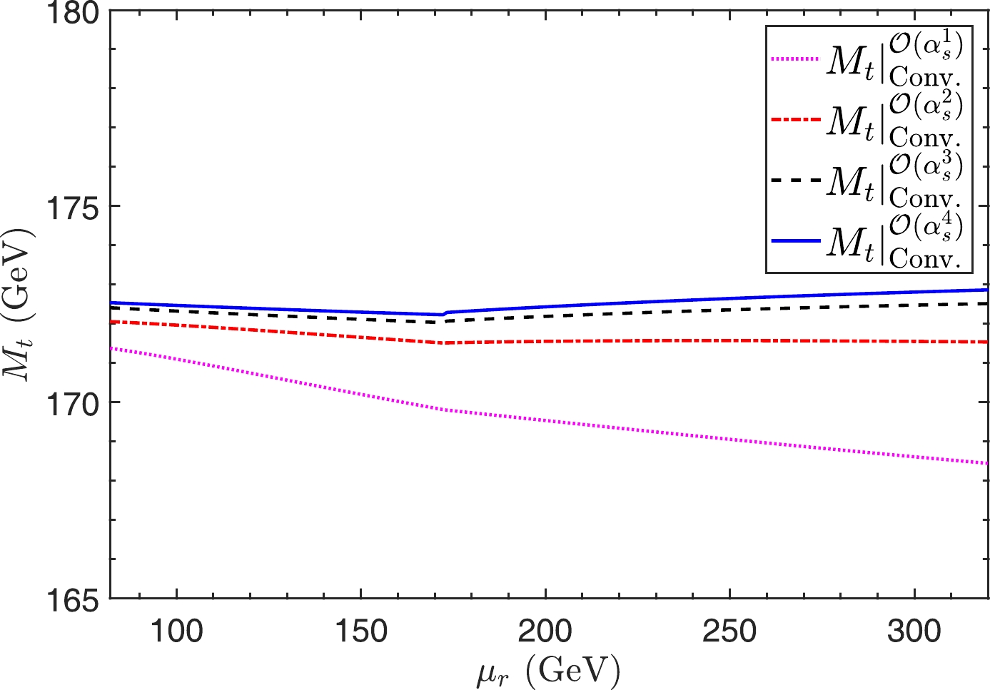
Figure 1. (color online) Top-quark OS mass
$ M_t $ versus renormalization scale ($ \mu_r $ ) under the conventional scale-setting approach up to different perturbative orders.$ \begin{aligned}[b] M_t|_{{\rm{Conv}}.}=\; &162.5^{-8.15}_{-0.83} +7.48^{+6.36}_{+0.62} + 1.60^{+1.80}_{+0.14} \\ & + 0.49^{+0.47}_{+0.03} + 0.19^{+0.14}_{+0.01} \\ = \;&172.26^{+0.62}_{-0.03} \; ({\rm{GeV}}), \end{aligned} $

(25) whose central values are those for
$ \mu_r={{\overline{m}}}_t({{\overline{m}}}_t) $ , and the scale uncertainties are estimated by varying$\mu_r \in [{{\overline{m}}}_t({{\overline{m}}}_t)/2, 2{{\overline{m}}}_t({{\overline{m}}}_t)]$ . The higher-order prediction of$ M_t $ is not a monotonic function of$ \mu_r $ , which leads to asymmetric uncertainty. By using another usual choice, i.e.,$\mu_r= 172.5$ GeV, and varying this value within the range of$[1/2 \times 172.5, 2 \times 172.5]$ , we obtain$ M_t=172.29^{+0.64}_{-0.06} $ GeV. The central value shifts from$ 172.26 $ GeV by$ +0.03 $ GeV, and its uncertainty remains asymmetric.We present
$ M_t $ under PMC scale-setting approach inFig. 2, which shows the top-quark OS mass$ M_t $ under the PMC single-scale approach up to different perturbative orders: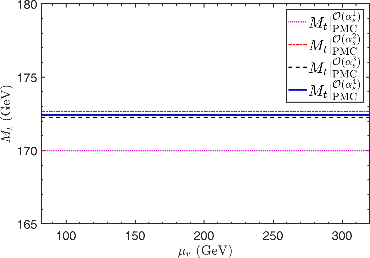
Figure 2. (color online) Top-quark OS mass
$ M_t $ versus renormalization scale ($ \mu_r $ ) under the PMC single-scale approach up to different perturbative orders.$ M_t|_{{\rm{PMC}}}^{{\rm{O}}(\alpha_s^n)}=\{170.01,172.66,172.27,172.41\} \; ({\rm{GeV}}) $

(26) for
$ n=1 $ , 2, 3, and 4, respectively. There is no renormalization scale ambiguity for the PMC prediction, and$ M_t $ quickly approaches its steady value. After applying the PMC, the perturbative nature of the$ M_t $ pQCD series is notably improved owing to the elimination of divergent renormalization terms. Moreover, the relative importance of the LO-terms: NLO-terms: N2LO-terms: N3LO-terms: N4LO-terms changes to 1: 4.79%: –1.15%: –0.15%: 0.07%. Up to N4LO-level, we have$ \begin{aligned}[b] M_t|_{{\rm{PMC}}}=\; &{{\overline{m}}}_t(Q_*)\{1+{\hat r}_{1,0}a_s(Q_*) + {\hat r}_{2,0}a_s^2(Q_*) \\ &+{\hat r}_{3,0}a_s^3(Q_*)+ {\hat r}_{4,0}a_s^4(Q_*)+{\rm{O}}[a^5_s(Q_*)]\} \\=\;& 166.49 + 7.97 - 1.92 - 0.25 + 0.12 \\ =\;& 172.41 \; ({\rm{GeV}}), \end{aligned} $

(27) where the PMC scale
$ Q_* $ can be established up to next-to-next-to-leading-log (N2LL) accuracy by using Eq. (17) as follows:$ \begin{aligned}[b] \ln\frac{Q^2_*}{{{\overline{m}}}_t^2(Q_*)}= \;&-68.73 a_s(Q_*)+247.483 a^2_s(Q_*) \\ &-6447.27 a^3_s(Q_*), \end{aligned} $

(28) which leads to
$ Q_*=123.3 $ GeV. Owing to its perturbative nature, we take the magnitude of the last known term as the unknown N3LL term in a conservative estimation of the unknown perturbative terms. Thus, we obtain a scale shift of$ \Delta Q_*=\left(^{+0.2}_{-0.3}\right) $ GeV, which leads to$ \begin{align} \Delta M_t|_{{\rm{PMC}}}=(^{+0.04}_{-0.03}) \; ({\rm{GeV}}). \end{align} $

(29) This uncertainty can be defined as the first type of residual scale dependence due to unknown higher-order terms [105]. Such residual scale dependence is distinct from the conventional scale ambiguities and is suppressed owing to the perturbative nature of the PMC scale. For the present case, the residual scale dependence expressed by Eq. (29) is much smaller than the conventional scale uncertainty presented in Eq. (25).
-
In pQCD calculations, the magnitude of unknown perturbative terms is also a major source of uncertainty. It is helpful to find a reliable prediction of the unknown higher-order terms. The Padé approximation approach (PAA) [106, 107] is a well-known method to estimate the
$ (n+1)_{{\rm{th}}} $ -order coefficient for a given$ n_{{\rm{th}}} $ -order perturbative series; this method has been tested on various known QCD results [108]. More explicitly, for the pQCD approximant$ \rho(Q^2)=c_1 a_s+c_2 a_s^2+c_3 a_s^3+c_4 a_s^4 $ , the preferable [n/n+1]-type PAA prediction [109] of the$ a_s^5 $ -terms of$ M_t $ under the conventional scale-setting approach is$\rho^{{\rm{N}}^{5}{\rm{LO}}}_{[1/2]} = \frac{2c_2 c_3 c_4-c_3^3-c_1 c_4^2} {c_2^2-c_1 c_3} a_s^5, $

(30) whereas the preferable [0/n-1]-type PAA prediction of the
$ a_s^5 $ -terms of$ M_t $ under the PMC scale-setting approach [92] is$ \rho^{{\rm{N}}^{5}{\rm{LO}}}_{[0/3]} = \frac{c_2^4-3c_1 c_2^2 c_3+2c_1^2 c_2 c_4+c_1^2 c_3^2} {c_1^3} a_s^5. $

(31) This uncertainty can be defined as the second type of residual scale dependence due to unknown higher-order terms. Then, our prediction of the magnitude of the N5LO-terms of top-quark OS mass
$ M_t $ is$ \Delta M_t\big|_{{\rm{Conv}}.}^{{\rm{N}}^{5}{\rm{LO}}}= \pm 0.08 \; ({\rm{GeV}}), $

(32) $ \Delta M_t\big|_{{\rm{PMC}}}^{{\rm{N}}^{5}{\rm{LO}}}= \pm 0.02 \; ({\rm{GeV}}). $

(33) Note that the conventional result is obtained by setting
$ \mu_r={{\overline{m}}}_t({{\overline{m}}}_t) $ , leading to numerical values that vary with the renormalization scale owing to the fact that the coefficients$ c_i $ are not fixed at each order. However, the PAA prediction of the PMC series exhibits no renormalization scale ambiguity, given that the PMC coefficients are scale-invariant.The combination of the two aforementioned residual scale dependences leads to a net perturbative uncertainty due to uncalculated higher-order terms under conventional and PMC scale-setting approaches:
$ {\Delta {M_t}} \big|_{{\rm{Conv}}.}^{{\rm{High}}\;{\rm{order}}} = (_{ - 0.09}^{ + 0.63})\;({\rm{GeV}}), $

(34) $ {\Delta {M_t}} \big|_{{\rm{PMC}}}^{{\rm{High}}\;{\rm{order}}} = \pm 0.04 \; ({\rm{GeV}}). $

(35) This shows that the PMC scale-invariant series provides a more accurate basis than the conventional scale-dependent series for estimating the uncertainty caused by uncalculated higher-order terms.
There are uncertainties from
$ \Delta\alpha_s(M_Z) $ and$ \Delta{{\overline{m}}}_t({{\overline{m}}}_t) $ . As an estimation, setting$ \Delta\alpha_s(M_Z)=\pm 0.0009 $ [75], we obtain$ \Delta M_t\big|_{{\rm{Conv}}.}^{\Delta\alpha_s(M_Z)} = \pm 0.09 \; ({\rm{GeV}}), $

(36) $ \Delta M_t \big|_{{\rm{PMC}}}^{\Delta\alpha_s(M_Z)} = (^{+0.10}_{-0.08}) \; ({\rm{GeV}}). $

(37) To estimate the uncertainty from the top-quark
$ \overline{{\rm{MS}}} $ mass, setting$ \Delta{{\overline{m}}}_t({{\overline{m}}}_t)=(^{+2.1}_{-1.5}) $ GeV, we obtain$ \Delta M_t \big|_{{\rm{Conv}}.}^{\Delta{{\overline{m}}}_t({{\overline{m}}}_t)}= (^{+2.20}_{-1.57}) \; ({\rm{GeV}}), $

(38) $ \Delta M_t \big|_{{\rm{PMC}}}^{\Delta{{\overline{m}}}_t({{\overline{m}}}_t)} = (^{+2.21}_{-1.57}) \; ({\rm{GeV}}). $

(39) This shows that the magnitude of
$ \Delta M_t $ is close to that of$ \Delta{{\overline{m}}}_t({{\overline{m}}}_t) $ .The final results for the top-quark OS mass are as follows:
$ M_t|_{{\rm{Conv}}.} = 172.26^{+2.29}_{-1.58} \; ({\rm{GeV}}), $

(40) $ M_t|_{{\rm{PMC}}}= 172.41^{+2.21}_{-1.57} \; ({\rm{GeV}}), $

(41) where the average uncertainties are squared with respect to those of
$ \Delta M_t|^{\text{High order}} $ ,$ \Delta M_t|^{\Delta\alpha_s(M_Z)} $ , and$ \Delta M_t|^{\Delta{{\overline{m}}}_t({{\overline{m}}}_t)} $ , respectively. Among these uncertainties, the one caused by$ \Delta{{\overline{m}}}_t({{\overline{m}}}_t) $ is dominant4 ; more accurate data are needed to suppress this uncertainty.We compare our results with experimental measurements [9, 75, 110] and some other theoretical predictions based on the analyses of top-pair production at hadronic colliders [46–48] in Table 1. All the predictions are consistent with each other within reasonable errors. Owing to the large input error of the top-quark
$ \overline{{\rm{MS}}} $ mass$ {{\overline{m}}}_t({{\overline{m}}}_t) $ , our results show larger uncertainty than those of Refs. [46–48]. Up to the present known N4LO level, the predictions under the PMC and conventional scale-setting approaches are both consistent with the latest experimental measurements [9].At present, the experimentally measured value of top-quark OS mass is more precise than that of the top-quark
$ \overline{{\rm{MS}}} $ mass. Thus, one can extract the$ \overline{{\rm{MS}}} $ mass$ {{\overline{m}}}_t({{\overline{m}}}_t) $ by inversely using Eq. (23) or the resultant PMC series. This is discussed in the following section. -
Using experimental results of OS mass is also a suitable approach for extracting the
$ \overline{{\rm{MS}}} $ mass$ {{\overline{m}}}_t({{\overline{m}}}_t) $ . The PDG [75] reports that the world average results of top-quark OS mass is$ M_t=172.5\pm 0.7 $ GeV, exhibiting a higher accuracy than that of the top-quark$ \overline{{\rm{MS}}} $ mass, i.e.,${{\overline{m}}}_t({{\overline{m}}}_t)= 162.5^{+2.1}_{-1.5}$ GeV.In the conventional scale-setting approach, one can extract the
$ \overline{{\rm{MS}}} $ mass$ {{\overline{m}}}_t({{\overline{m}}}_t) $ by using Eq. (23) and setting the renormalization scale$ \mu_r={{\overline{m}}}_t({{\overline{m}}}_t) $ :$ {{\overline{m}}}_t({{\overline{m}}}_t)|_{{\rm{Conv}}.}=162.73^{+0.67}_{-0.67} \; ({\rm{GeV}}), $

(42) where the central value is obtained by setting
$ M_t=172.5 $ GeV and the uncertainty is caused by$ \Delta M_t=\pm 0.7 $ GeV.Considering the uncertainty of the renormalization scale
$ \mu_r \in[\frac{1}{2}{{\overline{m}}}_t({{\overline{m}}}_t),2{{\overline{m}}}_t({{\overline{m}}}_t)] $ , we obtain$ {{\overline{m}}}_t({{\overline{m}}}_t)|_{{\rm{Conv}}.}=162.73^{+0.00}_{-1.16} \; ({\rm{GeV}}), $

(43) Thus, the conventional prediction is
$ {{\overline{m}}}_t({{\overline{m}}}_t)|_{{\rm{Conv}}.}=162.73^{+0.67}_{-1.34} \; ({\rm{GeV}}), $

(44) where the average uncertainty is squared with respect to that of
$ \Delta M_t=\pm 0.7 $ GeV and the renormalization scale$ \mu_r \in[\frac{1}{2}{{\overline{m}}}_t({{\overline{m}}}_t),2{{\overline{m}}}_t({{\overline{m}}}_t)] $ .In the PMC scale-setting approach, one can extract the
$ \overline{{\rm{MS}}} $ mass$ {{\overline{m}}}_t({{\overline{m}}}_t) $ by using the PMC series without renormalization scale uncertainty:$ \begin{aligned}[b] M_t=\;& {{\overline{m}}}_t(Q_*)\{1+{\hat r}_{1,0}a_s(Q_*) + {\hat r}_{2,0}a_s^2(Q_*) \\ &+{\hat r}_{3,0}a_s^3(Q_*)+ {\hat r}_{4,0}a_s^4(Q_*)+{\rm{O}}[a^5_s(Q_*)]\}, \end{aligned} $

(45) where the PMC scale
$ Q_* $ satisfies Eq. (28). Thus, the PMC prediction is$ {{\overline{m}}}_t({{\overline{m}}}_t)|_{{\rm{PMC}}}=163.08^{+0.66}_{-0.66} \; ({\rm{GeV}}), $

(46) where the central value is obtained by setting
$ M_t=172.5 $ GeV and the uncertainty is caused by$ \Delta M_t=\pm 0.7 $ GeV. It can be demonstrated that the PMC result predicted by Eq. (46) is more accurate than the conventional result predicted by Eq. (44). Finally, these results overlap with those of a previous study of ours,$ {{\overline{m}}}_t({{\overline{m}}}_t)=162.6^{+0.4}_{-0.4} $ GeV, obtained by using the RGE of$ \alpha_s $ alone [95] and the experimental result$ {{\overline{m}}}_t({{\overline{m}}}_t)=162.9\pm 0.5\pm 1.0^{+2.1}_{-1.2} $ GeV [10]. -
In the present paper, we have derived new degeneracy relations with the help of the RGEs involving both the β-function and quark mass anomalous dimension
$ \gamma_m $ -function, leading to improved PMC scale-setting procedures. Such procedures can be used to eliminate the conventional renormalization scale ambiguity of the fixed-order pQCD series under the$ \overline{{\rm{MS}}} $ running mass scheme, which simultaneously determines the correct magnitudes of$ \alpha_s $ and the$ \overline{{\rm{MS}}} $ running mass$ {{\overline{m}}}_q $ of the perturbative series with the help of RGEs. By applying such formulas, we have obtained a scale-invariant$ \overline{{\rm{MS}}} $ -on-shell quark mass relation. Consequently, we have determined the top-quark on-shell or$ \overline{{\rm{MS}}} $ mass without conventional renormalization scale ambiguity. By setting the top-quark$ \overline{{\rm{MS}}} $ mass as$ {{\overline{m}}}_t({{\overline{m}}}_t)=162.5^{+2.1}_{-1.5} $ given in PDG as an input, we obtain the top-quark OS mass$ M_t|_{{\rm{PMC}}}=172.41^{+2.21}_{-1.57} $ (GeV). It can be demonstrated that this result is characterized by a larger uncertainty than the experimental value, given that the input error$ \Delta{{\overline{m}}}_t({{\overline{m}}}_t) $ still exhibits a larger magnitude. We have also inversely determined the top-quark$ \overline{{\rm{MS}}} $ mass$ {{\overline{m}}}_t({{\overline{m}}}_t)=163.08^{+0.66}_{-0.66} $ by using the top-quark OS mass$ M_t=172.5\pm 0.7 $ GeV as input; the resultant prediction of the top-quark$ \overline{{\rm{MS}}} $ mass is more precise than the experimental value given in PDG.The accuracy of the pQCD prediction under the
$ \overline{{\rm{MS}}} $ running mass scheme strongly depends on the exact values of$ \alpha_s $ and$ {{\overline{m}}}_q $ . After applying the PMC, the correct values of the effective$ \alpha_s $ and$ {{\overline{m}}}_q $ can be determined simultaneously, resulting in a more convergent pQCD series that leads to a much smaller residual scale dependence. Thus, a reliable and precise pQCD prediction can be achieved. This is also a useful method to determine the bottom-quark OS mass and charm-quark OS mass in the future. -
We thank Sheng-Quan Wang, Jian-Ming Shen, Jun Zeng and Qing Yu for helpful discussions.
-
The general scale displacement relations of the strong coupling constant
$ a_s $ and quark running mass$ \overline{m}_q $ up to fourth-order are$ \begin{aligned}[b]\\[-3pt] a^k_s(\mu_r) =\;& a^k_s(\mu_\delta) + k \beta_0 \delta a^{k+1}_s(\mu_\delta) + k \bigg(\beta_1 \delta + \frac{k+1}{2}\beta_0^2 \delta^2 \bigg) a^{k+2}_s(\mu_\delta) \delta\\ &+ k\bigg[\beta_2 +\frac{2k+3}{2}\beta_0\beta_1 \delta^2 +\frac{(k+1)(k+2)}{3!}\beta_0^3 \delta^3 \bigg]a^{k+3}_s(\mu_\delta)+{\rm{O}}[a^{k+4}_s(\mu_\delta)]. \end{aligned}\tag{A1}$ 
$\begin{aligned}[b] {{\overline{m}}}_q^n(\mu_r)=\;& {{\overline{m}}}_q^n(\mu_\delta)\bigg\{1+n\gamma_0\delta a_s+\bigg[\frac{1}{2} \left(n\beta_0\gamma_0+n^2\gamma_0^2\right)\delta^2 +n\gamma_1\delta\bigg]a_s^2 +\bigg[n\gamma_2\delta+\frac{1}{2} (2n\beta_0\gamma_1 \\ &+ n\beta_1\gamma_0+2n^2\gamma_0\gamma_1)\delta^2+\frac{1}{3!}\bigg(2n\beta_0^2\gamma_0 +3n^2\beta_0\gamma_0^2+n^3\gamma_0^3\bigg)\delta^3\bigg]a_s^3 +\bigg[n\gamma_3\delta \\ &+\frac{1}{2}\bigg(3n\beta_0\gamma_2+2n \beta_1\gamma_1+n\beta_2\gamma_0+2n^2\gamma_0\gamma_2+n^2\gamma_1^2\bigg) \delta^2 +\frac{1}{3!} \bigg(6n\beta_0^2\gamma_1+5n\beta_0\beta_1\gamma_0 \\ &+9n^2\beta_0\gamma_0\gamma_1+3 n^2\beta_1\gamma_0^2+3n^3\gamma_0^2\gamma_1\bigg) \delta ^3 +\frac{1}{4!} \bigg(6n\beta_0^3\gamma_0+11n^2\beta_0^2\gamma_0^2+6n^3\beta_0\gamma_0^3 + n^4\gamma_0^4\bigg)\delta ^4 \bigg]a_s^4+{\rm{O}}(a^5_s)\bigg\}. \end{aligned}\tag{A2} $

-
$ \begin{aligned}[b] \rho_\delta(Q^2)=\;& r_0 {{\overline{m}}}_q^n(\mu_{\delta}) \Big\{1+(r_1+n \gamma_0 \delta)a_s(\mu_{\delta}) + \Big[r_2+\beta_0r_1\delta+n(\gamma_1+\gamma_0r_1)\delta+\frac{n}{2}\beta_0\gamma_0\delta^2+\frac{n^2}{2}\gamma_0^2\delta^2 \Big] a^2_s(\mu_{\delta})\\ &+ \Big[r_3+\beta_1r_1\delta+2\beta_0r_2\delta+\beta_0^2r_1\delta^2+n(\gamma_2+\gamma_0r_2+\gamma_1r_1)\delta+n\beta_0 \Big(\gamma_1+\frac{3\gamma_0r_1}{2}\Big)\delta^2+\frac{n}{2}\beta_1\gamma_0\delta^2+\frac{n}{3}\beta_0^2\gamma_0\delta^3\\ &+n^2 \Big(\gamma_1\gamma_0+\frac{\gamma_0^2r_1}{2}\Big) \delta^2+\frac{n^2}{2}\beta_0\gamma_0^2\delta^3+\frac{n^3}{6}\gamma_0^3\delta^3 \Big] a^3_s(\mu_{\delta})+ \Big[r_4+(2\beta_1r_2+\beta_2r_1)\delta+3\beta_0r_3\delta+\frac{5}{2}\beta_0\beta_1r_1\delta^2+3\beta_0^2r_2\delta^2\\ &+\beta_0^3r_1\delta^3+n(\gamma_3+\gamma_0r_3+\gamma_1r_2+\gamma_2r_1)\delta+n\beta_0\Big(\frac{3\gamma_2}{2}+\frac{5\gamma_0r_2}{2}+2\gamma_1r_1\Big)\delta^2+ n \Big(\frac{\beta_2\gamma_0}{2}+\beta_1\gamma_1+\frac{3}{2}\beta_1\gamma_0r_1\Big)\delta^2\\ &+n\beta_0^2 \Big(\gamma_1+\frac{11\gamma_0r_1}{6}\Big)\delta^3+\frac{5n}{6}\beta_0\beta_1\gamma_0\delta^3+\frac{n}{4}\beta_0^3\gamma_0\delta^4+n^2 \Big(\gamma_2\gamma_0+\frac{\gamma_1^2}{2}+\frac{\gamma_0^2r_2}{2}+\gamma_1\gamma_0r_1\Big)\delta^2+n^2\beta_0 \Big(\frac{3\gamma_1\gamma_0}{2}+\gamma_0^2r_1\Big)\delta^3\\ &+\frac{n^2}{2}\beta_1\gamma_0^2\delta^3+\frac{11n^2}{24}\beta_0^2\gamma_0^2\delta^4+n^3 \Big(\frac{\gamma_1\gamma_0^2}{2}+\frac{\gamma_0^3r_1}{6}\Big)\delta^3+\frac{n^3}{4}\beta_0\gamma_0^3\delta^4+\frac{n^4}{24}\gamma_0^4\delta^4 \Big] a^4_s(\mu_{\delta})+{\rm{O}}[a^5_s(\mu_{\delta})]\Big\}. \end{aligned}\tag{B1} $

-
$ \begin{aligned}[b] \rho(Q^2)=\;& r_0 {{\overline{m}}}_q^n(\mu_r)\Big\{1+ \Big({\hat r}_{1,0}+n\gamma_0\ln\frac{\mu_r^2}{Q^2}\Big) a_s(\mu_r) + \Big[{\hat r}_{2,0}+\beta_0{\hat r}_{2,1}+n\gamma_0{\hat r}_{2,1} +(\beta_0{\hat r}_{1,0}+n\gamma_1+n\gamma_0{\hat r}_{1,0})\ln\frac{\mu_r^2}{Q^2}\\ &+\frac{1}{2}(n\beta_0\gamma_0+n^2\gamma_0^2)\ln^2\frac{\mu_r^2}{Q^2}\Big] a^2_s(\mu_r) +\{{\hat r}_{3,0}+\beta_1{\hat r}_{2,1}+2\beta_0{\hat r}_{3,1}+\beta_0^2{\hat r}_{3,2}+n(\gamma_0{\hat r}_{3,1}+\gamma_1{\hat r}_{2,1})+\frac{3n}{2}\beta_0\gamma_0{\hat r}_{3,2}\\ &+\frac{n^2}{2}\gamma_0^2{\hat r}_{3,2}+[\beta_1{\hat r}_{1,0}+2\beta_0{\hat r}_{2,0}+2\beta_0^2{\hat r}_{2,1}+n(\gamma_2+\gamma_1{\hat r}_{1,0}+\gamma_0{\hat r}_{2,0}+3\beta_0\gamma_0{\hat r}_{2,1}+ n\gamma_0^2{\hat r}_{2,1})]\ln\frac{\mu_r^2}{Q^2}\\ &+ \Big[\beta_0^2{\hat r}_{1,0}+n(\beta_0\gamma_1+\frac{1}{2}\beta_1\gamma_0+\frac{3}{2}\beta_0\gamma_0{\hat r}_{1,0})+n^2(\gamma_0\gamma_1 +\frac{1}{2}\gamma_0^2{\hat r}_{1,0})\Big]\ln^2\frac{\mu_r^2}{Q^2}+\frac{1}{6}(2n\beta_0^2\gamma_0+3n^2\beta_0\gamma_0^2+n^3\gamma_0^3)\ln^3\frac{\mu_r^2}{Q^2}\Big\} a^3_s(\mu_r) \\ &+ \Big\{{\hat r}_{4,0}+\beta_2{\hat r}_{2,1}+2\beta_1{\hat r}_{3,1}+3\beta_0{\hat r}_{4,1}+\frac{5}{2}\beta_0\beta_1{\hat r}_{3,2}+3\beta_0^2{\hat r}_{4,2}+\beta_0^3{\hat r}_{4,3} + n\beta_0 \Big(2\gamma_1{\hat r}_{3,2}+\frac{5}{2}\gamma_0{\hat r}_{4,2}\Big)\\ &+n \Big(\frac{3}{2}\beta_1\gamma_0{\hat r}_{3,2}+\gamma_2{\hat r}_{2,1}+\gamma_1{\hat r}_{3,1}+\gamma_0{\hat r}_{4,1}\Big)+\frac{11n}{6}\beta_0^2\gamma_0{\hat r}_{4,3}+n^2 \Big(\frac{\gamma_0^2{\hat r}_{4,2}}{2}+\gamma_1\gamma_0{\hat r}_{3,2}\Big)+n^2\beta_0\gamma_0^2{\hat r}_{4,3}+\frac{n^3}{6}\gamma_0^3{\hat r}_{4,3}\\ &+ \Big[\beta_2{\hat r}_{1,0}+2\beta_1{\hat r}_{2,0}+3\beta_0{\hat r}_{3,0}+6\beta_0^2{\hat r}_{3,1}+3\beta_0^3{\hat r}_{3,2}+5\beta_1\beta_0{\hat r}_{2,1}+n \Big(\gamma_3+\gamma_2{\hat r}_{1,0}+\gamma_1{\hat r}_{2,0}+\gamma_0{\hat r}_{3,0}+\frac{11}{2}\beta_0^2\gamma_0{\hat r}_{3,2}\\ &+4\beta_0\gamma_1{\hat r}_{2,1}+5\beta_0\gamma_0{\hat r}_{3,1}+3\beta_1\gamma_0{\hat r}_{2,1}\Big)+n^2(3\beta_0\gamma_0^2{\hat r}_{3,2}+2\gamma_0\gamma_1{\hat r}_{2,1})+\frac{n^3}{2}\gamma_0^3{\hat r}_{3,2}\Big]\ln\frac{\mu_r^2}{Q^2}\\ &+ \Big[3\beta_0^2{\hat r}_{2,0}+3\beta_0^3{\hat r}_{2,1}+\frac{5}{2}\beta_0\beta_1{\hat r}_{1,0}+n \Big(\frac{3}{2}\beta_0\gamma_2+\beta_1\gamma_1+\frac{1}{2}\beta_2\gamma_0+\frac{3}{2}\beta_1\gamma_0{\hat r}_{1,0}+\frac{11}{2}\beta_0^2\gamma_0{\hat r}_{2,1}+2\beta_0\gamma_1{\hat r}_{1,0}+\frac{5}{2}\beta_0\gamma_0{\hat r}_{2,0}\Big)\\ &+ n^2\Big(\frac{1}{2}\gamma_1^2+\gamma_0\gamma_2+\gamma_0\gamma_1{\hat r}_{1,0}+\frac{1}{2}\gamma_0^2{\hat r}_{2,0}+3\beta_0\gamma_0^2{\hat r}_{2,1}\Big)+\frac{n^3}{2}\gamma_0^3{\hat r}_{2,1}\Big]\ln^2\frac{\mu_r^2}{Q^2}+ \Big[\beta_0^3{\hat r}_{1,0}+n\Big(\beta_0^2\gamma_1+\frac{11}{6}\beta_0^2\gamma_0{\hat r}_{1,0}+\frac{5}{6}\beta_0\beta_1\gamma_0\Big)\\ &+n^2\Big(\beta_0\gamma_0^2{\hat r}_{1,0}+\frac{1}{2}\beta_1\gamma_0^2+\frac{3}{2}\beta_0\gamma_0\gamma_1\Big)+n^3\Big(\frac{1}{6}\gamma_0^3{\hat r}_{1,0}+\frac{1}{2}\gamma_0^2\gamma_1\Big)\Big]\ln^3\frac{\mu_r^2}{Q^2}\\&+\Big(\frac{n}{4}\beta_0^3\gamma_0+\frac{11n^2}{24}\beta_0^2\gamma_0^2+\frac{n^3}{4}\beta_0\gamma_0^3+\frac{n^4}{24}\gamma_0^4\Big)\ln^4\frac{\mu_r^2}{Q^2}\Big\} a^4_s(\mu_r)+{\rm{O}}[a^5_s(\mu_r)\Big]\Big\}. \end{aligned}\tag{C1} $

-
$ \begin{aligned}[b] r_3(\mu_r^2/Q^2)= {\hat r}_{3,0}+\beta_1{\hat r}_{2,1}+2\beta_0{\hat r}_{3,1}+\beta_0^2{\hat r}_{3,2}+n(\gamma_0{\hat r}_{3,1}+\gamma_1{\hat r}_{2,1})+\frac{3n}{2}\beta_0\gamma_0{\hat r}_{3,2}+\frac{n^2}{2}\gamma_0^2{\hat r}_{3,2}+[\beta_1{\hat r}_{1,0}+2\beta_0{\hat r}_{2,0}+2\beta_0^2{\hat r}_{2,1} \end{aligned} $

$ \begin{aligned}[b] \quad\quad\quad\quad\quad\quad &+n(\gamma_2+\gamma_1{\hat r}_{1,0}+\gamma_0{\hat r}_{2,0}+3\beta_0\gamma_0{\hat r}_{2,1}+ n\gamma_0^2{\hat r}_{2,1})]\ln\frac{\mu_r^2}{Q^2}+[\beta_0^2{\hat r}_{1,0}+n(\beta_0\gamma_1+\frac{1}{2}\beta_1\gamma_0+\frac{3}{2}\beta_0\gamma_0{\hat r}_{1,0})\\ &+n^2(\gamma_0\gamma_1+\frac{1}{2}\gamma_0^2{\hat r}_{1,0})]\ln^2\frac{\mu_r^2}{Q^2}+\frac{1}{6}(2n\beta_0^2\gamma_0+3n^2\beta_0\gamma_0^2+n^3\gamma_0^3)\ln^3\frac{\mu_r^2}{Q^2}, \end{aligned}\tag{D1} $

$\begin{aligned}[b] r_4(\mu_r^2/Q^2)=\;& {\hat r}_{4,0}+\beta_2{\hat r}_{2,1}+2\beta_1{\hat r}_{3,1}+3\beta_0{\hat r}_{4,1}+\frac{5}{2}\beta_0\beta_1{\hat r}_{3,2}+3\beta_0^2{\hat r}_{4,2}+\beta_0^3{\hat r}_{4,3} + n\beta_0 \Big(2\gamma_1{\hat r}_{3,2}+\frac{5}{2}\gamma_0{\hat r}_{4,2}\Big)\\ &+n\Big(\frac{3}{2}\beta_1\gamma_0{\hat r}_{3,2}+\gamma_2{\hat r}_{2,1}+\gamma_1{\hat r}_{3,1}+\gamma_0{\hat r}_{4,1}\Big)+\frac{11n}{6}\beta_0^2\gamma_0{\hat r}_{4,3}+n^2\Big(\frac{\gamma_0^2{\hat r}_{4,2}}{2}+\gamma_1\gamma_0{\hat r}_{3,2}\Big)+n^2\beta_0\gamma_0^2{\hat r}_{4,3}+\frac{n^3}{6}\gamma_0^3{\hat r}_{4,3}\\ &+ \Big[\beta_2{\hat r}_{1,0}+2\beta_1{\hat r}_{2,0}+3\beta_0{\hat r}_{3,0}+6\beta_0^2{\hat r}_{3,1}+3\beta_0^3{\hat r}_{3,2}+5\beta_1\beta_0{\hat r}_{2,1}+n\Big(\gamma_3+\gamma_2{\hat r}_{1,0}+\gamma_1{\hat r}_{2,0}+\gamma_0{\hat r}_{3,0}\\ &+\frac{11}{2}\beta_0^2\gamma_0{\hat r}_{3,2}+4\beta_0\gamma_1{\hat r}_{2,1}+5\beta_0\gamma_0{\hat r}_{3,1}+3\beta_1\gamma_0{\hat r}_{2,1}\Big)+n^2(3\beta_0\gamma_0^2{\hat r}_{3,2}+2\gamma_0\gamma_1{\hat r}_{2,1})+\frac{n^3}{2}\gamma_0^3{\hat r}_{3,2}\Big]\ln\frac{\mu_r^2}{Q^2}\\ &+ \Big[3\beta_0^2{\hat r}_{2,0}+3\beta_0^3{\hat r}_{2,1}+\frac{5}{2}\beta_0\beta_1{\hat r}_{1,0}+n\Big(\frac{3}{2}\beta_0\gamma_2+\beta_1\gamma_1+\frac{1}{2}\beta_2\gamma_0+\frac{3}{2}\beta_1\gamma_0{\hat r}_{1,0}+\frac{11}{2}\beta_0^2\gamma_0{\hat r}_{2,1}+2\beta_0\gamma_1{\hat r}_{1,0}+\frac{5}{2}\beta_0\gamma_0{\hat r}_{2,0}\Big)\\ &+ n^2\Big(\frac{1}{2}\gamma_1^2+\gamma_0\gamma_2+\gamma_0\gamma_1{\hat r}_{1,0}+\frac{1}{2}\gamma_0^2{\hat r}_{2,0}+3\beta_0\gamma_0^2{\hat r}_{2,1}\Big)+\frac{n^3}{2}\gamma_0^3{\hat r}_{2,1}\Big]\ln^2\frac{\mu_r^2}{Q^2} +\Big[\beta_0^3{\hat r}_{1,0}+n\Big(\beta_0^2\gamma_1+\frac{11}{6}\beta_0^2\gamma_0{\hat r}_{1,0}\\ &+\frac{5}{6}\beta_0\beta_1\gamma_0\Big)+n^2\Big(\beta_0\gamma_0^2{\hat r}_{1,0}+\frac{1}{2}\beta_1\gamma_0^2+\frac{3}{2}\beta_0\gamma_0\gamma_1\Big)+n^3\Big(\frac{1}{6}\gamma_0^3{\hat r}_{1,0}+\frac{1}{2}\gamma_0^2\gamma_1\Big)\Big]\ln^3\frac{\mu_r^2}{Q^2}\\ &+\Big(\frac{n}{4}\beta_0^3\gamma_0+\frac{11n^2}{24}\beta_0^2\gamma_0^2+\frac{n^3}{4}\beta_0\gamma_0^3+\frac{n^4}{24}\gamma_0^4\Big)\ln^4\frac{\mu_r^2}{Q^2}. \end{aligned}\tag{D2} $

-
It is possible to infer some degenerate relations from Eq. (B1). For example, the coefficients of
$ \beta_0 a_s^2 $ ,$ n\gamma_0 a_s^2 $ ,$ \beta_1 a_s^3 $ ,$ n\gamma_1 a_s^3 $ ,$ \beta_2 a_s^4 $ , and$ n\gamma_2 a_s^4 $ are the same, namely$ r_1\delta $ . By substituting$ r_i\delta^j \rightarrow r_{i+j,j} $ , the expression for ρ at$ \mu_r=Q $ can be rewritten as$\begin{aligned}[b] \rho(Q^2)=\;& r_0 {{\overline{m}}}_q^n(Q)\Big\{1+{\hat r}_{1,0}a_s(Q) +\left({\hat r}_{2,0}+\beta_0{\hat r}_{2,1}+n\gamma_0{\hat r}_{2,1}\right)a^2_s(Q)+\Big[{\hat r}_{3,0}+\beta_1{\hat r}_{2,1}+2\beta_0{\hat r}_{3,1}+\beta_0^2{\hat r}_{3,2}+n(\gamma_0{\hat r}_{3,1}+\gamma_1{\hat r}_{2,1})+\frac{3n}{2}\beta_0\gamma_0{\hat r}_{3,2}\\ &+\frac{n^2}{2}\gamma_0^2{\hat r}_{3,2}\Big]a^3_s(Q)+ \Big[{\hat r}_{4,0}+\beta_2{\hat r}_{2,1}+2\beta_1{\hat r}_{3,1}+3\beta_0{\hat r}_{4,1}+\frac{5}{2}\beta_0\beta_1{\hat r}_{3,2}+3\beta_0^2{\hat r}_{4,2}+\beta_0^3{\hat r}_{4,3}+n\beta_0 \Big(2\gamma_1{\hat r}_{3,2}+\frac{5}{2}\gamma_0{\hat r}_{4,2}\Big)\\ &+n\Big(\frac{3}{2}\beta_1\gamma_0{\hat r}_{3,2}+\gamma_2{\hat r}_{2,1}+\gamma_1{\hat r}_{3,1}+\gamma_0{\hat r}_{4,1}\Big)+\frac{11n}{6}\beta_0^2\gamma_0{\hat r}_{4,3}+n^2\Big(\frac{\gamma_0^2{\hat r}_{4,2}}{2}+\gamma_1\gamma_0{\hat r}_{3,2}\Big)\\ &+n^2\beta_0\gamma_0^2{\hat r}_{4,3}+\frac{n^3}{6}\gamma_0^3{\hat r}_{4,3}\Big]a^4_s(Q)+{\rm{O}}[a^5_s(Q)]\Big\}. \end{aligned}\tag{E1} $

A pQCD calculation prediction for a physical observable at
$ \mu_r=Q $ is$ \rho(Q^2)= r_0{{\overline{m}}}_q^n(Q) \bigg[1+\sum\limits_{k=1}^{\infty} \left(\sum\limits_{l=0}^{k-1} c_{k,l} n_f^{l}\right) a_s^k(Q)\bigg]. \tag{E2} $

Comparing Eq. (E1) with Eq. (E2) for each order, the coefficients of the
$ n_f $ series can be matched to the$ r_{i,j} $ coefficients in a unique manner. More explicitly, one can derive the relations between$ c_{k,l} $ and$ r_{i,j} $ by using the$ \beta_i $ and$ \gamma_i $ coefficients given in [70, 72]; e.g., it is easy to find that$ {\hat r}_{1,0}=c_{1,0} $ . Substituting$ \beta_0=11-\frac{2}{3}n_f $ and$ \gamma_0=4 $ into the$ a_s^2 $ -order coefficient of Eq. (E1), we can find$ r_{2,0} $ and$ r_{2,1} $ :$ c_{2,0}+c_{2,1}n_f={\hat r}_{2,0}+\left(11-\frac{2}{3}n_f\right){\hat r}_{2,1}+4n{\hat r}_{2,1}, \tag{E3} $

which leads to
$ {\hat r}_{1,0}= c_{1,0}, \tag{E4} $

$ {\hat r}_{2,0}= c_{2,0}+\left(6n+\frac{33}{2}\right)c_{2,1},\; {\hat r}_{2,1}=-\frac{3}{2}c_{2,1}. \tag{E5} $

Following the same procedures, one can derive these relations up to any order. In the present paper, we use the relations up to fourth order:
$ \begin{aligned}[b]{\hat r}_{3,0}=\;&c_{3,0}+\left(3n+\frac{33}{2}\right)c_{3,1}+\left(9n^2+99n+\frac{1089}{4}\right)c_{3,2}-\left(10n^2+11n+\frac{321}{2}\right)c_{2,1},\\ {\hat r}_{3,1}=\;& -\frac{3}{4}c_{3,1}-\frac{27n+99}{4}c_{3,2}+\frac{10n+57}{4}c_{2,1},\; {\hat r}_{3,2}=\frac{9}{4}c_{3,2}, \end{aligned}\tag{E6} $

$ \begin{aligned}[b]{\hat r}_{4,0}=\;& c_{4,0}+\left(2n+\frac{33}{2}\right)c_{4,1}+\left(4n^2+66n+\frac{1089}{4}\right)c_{4,2}+\Bigg(8n^3+198n^2+\frac{3267n}{2}+\frac{35937}{8}\Bigg)c_{4,3}\\ &-\left(\frac{50n^3}{3}+185n^2+\frac{2595n}{2}+\frac{10593}{2}\right)c_{3,2}-\left(\frac{10n^2}{3}+15n+\frac{321}{2}\right)c_{3,1}\\ &+\left(\frac{20n^3}{27}-160\zeta_3n^2-\frac{2411n^2}{9}-\frac{860n}{3}-1320\zeta_3n+\frac{11675}{16}\right)c_{2,1}, \end{aligned}\tag{E7} $

$ \begin{aligned}[b]{\hat r}_{4,1}=\;& -\frac{1}{2}c_{4,1}-\frac{1}{2}\left(5n+33\right)c_{4,2}-\left(\frac{19n^2}{2}+\frac{495n}{4}+\frac{3267}{8}\right)c_{4,3}+\left(\frac{5n}{6}+\frac{19}{2}\right)c_{3,1}+\left(\frac{85n^2}{6}+\frac{401n}{4}+\frac{4113}{8}\right)c_{3,2}\\ &+\left(\frac{100n^2}{27}+40\zeta_3n+\frac{2467n}{72}-\frac{479}{4}\right)c_{2,1}, \end{aligned}\tag{E8} $

$ {\hat r}_{4,2}= \frac{3}{4}c_{4,2}+\left(\frac{33n}{4}+\frac{297}{8}\right)c_{4,3}-\left(5n+\frac{285}{8}\right)c_{3,2}+\left(\frac{325}{48}-\frac{35n}{18}\right)c_{2,1}, \tag{E9} $

$ {\hat r}_{4,3} = -\frac{27}{8}c_{4,3}. \tag{E10} $

Note that one must treat the
$ n_f $ terms which are not related to renormalization of the running coupling and running mass as part of the conformal coefficient; e.g., the$ n_f $ terms coming from the light-by-light diagrams in QCD belong to the conformal series. The contributions of light-by-light diagrams are always established separately, given that the light-by-light diagrams can be easily distinguished from the other Feynman diagrams. -
$ \begin{aligned}[b]r_{\rm 3, NonConf.}(Q_*)= \beta_1{\hat r}_{2,1}+2\beta_0{\hat r}_{3,1}+\beta_0^2{\hat r}_{3,2}+n(\gamma_0{\hat r}_{3,1}+\gamma_1{\hat r}_{2,1})+\frac{3n}{2}\beta_0\gamma_0{\hat r}_{3,2}+\frac{n^2}{2}\gamma_0^2{\hat r}_{3,2}+\Big[\beta_1{\hat r}_{1,0}+2\beta_0{\hat r}_{2,0}+2\beta_0^2{\hat r}_{2,1} \end{aligned} $

$ \begin{aligned}[b]\qquad\qquad\qquad &+n(\gamma_2+\gamma_1{\hat r}_{1,0}+\gamma_0{\hat r}_{2,0}+3\beta_0\gamma_0{\hat r}_{2,1}+ n\gamma_0^2{\hat r}_{2,1})\Big]\ln\frac{Q_*^2}{Q^2}+\Big[\beta_0^2{\hat r}_{1,0}+n\Big(\beta_0\gamma_1+\frac{1}{2}\beta_1\gamma_0+\frac{3}{2}\beta_0\gamma_0{\hat r}_{1,0}\Big)\\ &+n^2(\gamma_0\gamma_1+\frac{1}{2}\gamma_0^2{\hat r}_{1,0})\Big]\ln^2\frac{Q_*^2}{Q^2}+\frac{1}{6}(2n\beta_0^2\gamma_0+3n^2\beta_0\gamma_0^2+n^3\gamma_0^3)\ln^3\frac{Q_*^2}{Q^2}, \end{aligned}\tag{F1} $

$ \begin{aligned}[b]r_{\rm 4, NonConf.}(Q_*)=\;& \beta_2{\hat r}_{2,1}+2\beta_1{\hat r}_{3,1}+3\beta_0{\hat r}_{4,1}+\frac{5}{2}\beta_0\beta_1{\hat r}_{3,2}+3\beta_0^2{\hat r}_{4,2}+\beta_0^3{\hat r}_{4,3} + n\beta_0\Big(2\gamma_1{\hat r}_{3,2}+\frac{5}{2}\gamma_0{\hat r}_{4,2}\Big)\\ &+n\Big(\frac{3}{2}\beta_1\gamma_0{\hat r}_{3,2}+\gamma_2{\hat r}_{2,1}+\gamma_1{\hat r}_{3,1}+\gamma_0{\hat r}_{4,1}\Big)+\frac{11n}{6}\beta_0^2\gamma_0{\hat r}_{4,3}+n^2\Big(\frac{\gamma_0^2{\hat r}_{4,2}}{2}+\gamma_1\gamma_0{\hat r}_{3,2}\Big)+n^2\beta_0\gamma_0^2{\hat r}_{4,3}\\ &+\frac{n^3}{6}\gamma_0^3{\hat r}_{4,3}+ \Big[\beta_2{\hat r}_{1,0}+2\beta_1{\hat r}_{2,0}+3\beta_0{\hat r}_{3,0}+6\beta_0^2{\hat r}_{3,1}+3\beta_0^3{\hat r}_{3,2}+5\beta_1\beta_0{\hat r}_{2,1}+n(\gamma_3+\gamma_2{\hat r}_{1,0}+\gamma_1{\hat r}_{2,0}\\ &+\gamma_0{\hat r}_{3,0}+\frac{11}{2}\beta_0^2\gamma_0{\hat r}_{3,2}+4\beta_0\gamma_1{\hat r}_{2,1}+5\beta_0\gamma_0{\hat r}_{3,1}+3\beta_1\gamma_0{\hat r}_{2,1})+n^2(3\beta_0\gamma_0^2{\hat r}_{3,2}+2\gamma_0\gamma_1{\hat r}_{2,1})+\frac{n^3}{2}\gamma_0^3{\hat r}_{3,2}\Big]\ln\frac{Q_*^2}{Q^2}\\ &+\Big[3\beta_0^2{\hat r}_{2,0}+3\beta_0^3{\hat r}_{2,1}+\frac{5}{2}\beta_0\beta_1{\hat r}_{1,0}+n\Big(\frac{3}{2}\beta_0\gamma_2+\beta_1\gamma_1+\frac{1}{2}\beta_2\gamma_0+\frac{3}{2}\beta_1\gamma_0{\hat r}_{1,0}+\frac{11}{2}\beta_0^2\gamma_0{\hat r}_{2,1}+2\beta_0\gamma_1{\hat r}_{1,0}+\frac{5}{2}\beta_0\gamma_0{\hat r}_{2,0}\Big)\\ &+ n^2\Big(\frac{1}{2}\gamma_1^2+\gamma_0\gamma_2+\gamma_0\gamma_1{\hat r}_{1,0}+\frac{1}{2}\gamma_0^2{\hat r}_{2,0}+3\beta_0\gamma_0^2{\hat r}_{2,1}\Big)+\frac{n^3}{2}\gamma_0^3{\hat r}_{2,1}\Big]\ln^2\frac{Q_*^2}{Q^2}\\ &+\Big[\beta_0^3{\hat r}_{1,0}+n\Big(\beta_0^2\gamma_1+\frac{11}{6}\beta_0^2\gamma_0{\hat r}_{1,0}+\frac{5}{6}\beta_0\beta_1\gamma_0\Big)+n^2\Big(\beta_0\gamma_0^2{\hat r}_{1,0}+\frac{1}{2}\beta_1\gamma_0^2+\frac{3}{2}\beta_0\gamma_0\gamma_1\Big)\\ &+n^3\Big(\frac{1}{6}\gamma_0^3{\hat r}_{1,0}+\frac{1}{2}\gamma_0^2\gamma_1\Big)\Big]\ln^3\frac{Q_*^2}{Q^2}+\Big(\frac{n}{4}\beta_0^3\gamma_0+\frac{11n^2}{24}\beta_0^2\gamma_0^2+\frac{n^3}{4}\beta_0\gamma_0^3+\frac{n^4}{24}\gamma_0^4\Big)\ln^4\frac{Q_*^2}{Q^2}. \end{aligned}\tag{F2} $

-
$\begin{aligned}[b] S_3=\;& {\hat r}_{1,0}{\hat r}_{3,1}-{\hat r}_{1,0}^2{\hat r}_{2,1}+{\hat r}_{2,0}{\hat r}_{2,1}-{\hat r}_{4,1}+\frac{n\gamma_0}{2}({\hat r}_{2,1}^2+{\hat r}_{1,0}{\hat r}_{3,2}-{\hat r}_{4,2})-\frac{n\gamma_1{\hat r}_{3,2}}{2}-\frac{n^2\gamma_0^2{\hat r}_{4,3}}{6} -\frac{\beta_2{\hat r}_{2,1}}{n\gamma_0}\\ &+\beta_1\Big(\frac{\gamma_1{\hat r}_{2,1}}{n\gamma_0^2}+\frac{2{\hat r}_{1,0}{\hat r}_{2,1}-2{\hat r}_{3,1}}{n\gamma_0}-\frac{3{\hat r}_{3,2}}{2}\Big)+\beta_0\beta_1\Big(\frac{2{\hat r}_{1,0}{\hat r}_{2,1}}{n^2\gamma_0^2}-\frac{5{\hat r}_{3,2}}{2n\gamma_0}\Big) +\beta_0\bigg(\frac{5{\hat r}_{2,1}^2}{2}-n\gamma_0{\hat r}_{4,3}-\frac{5{\hat r}_{4,2}}{2}+2{\hat r}_{1,0}{\hat r}_{3,2}-\frac{\gamma_1^2{\hat r}_{2,1}}{n\gamma_0^3}\\ &+\frac{\gamma_2{\hat r}_{2,1}+2\gamma_1{\hat r}_{3,1}-2\gamma_1{\hat r}_{1,0}{\hat r}_{2,1}}{n\gamma_0^2} -\frac{n\gamma_1{\hat r}_{3,2}+6{\hat r}_{2,1}{\hat r}_{1,0}^2-6{\hat r}_{3,1}{\hat r}_{1,0}-6{\hat r}_{2,0}{\hat r}_{2,1}+6{\hat r}_{4,1}}{2n\gamma_0}\bigg)+\beta_0^2\bigg(\frac{7{\hat r}_{2,1}^2+5{\hat r}_{1,0}{\hat r}_{3,2}-6{\hat r}_{4,2}}{2n\gamma_0}\\ &+\frac{n\gamma_1{\hat r}_{3,2}-3{\hat r}_{2,1}{\hat r}_{1,0}^2+2{\hat r}_{3,1}{\hat r}_{1,0}+2{\hat r}_{2,0}{\hat r}_{2,1}}{n^2\gamma_0^2}-\frac{2\gamma_1{\hat r}_{1,0}{\hat r}_{2,1}}{n^3\gamma_0^3}-\frac{11{\hat r}_{4,3}}{6}\bigg)+\beta_0^3\Big(\frac{3{\hat r}_{2,1}^2+2{\hat r}_{1,0}{\hat r}_{3,2}}{2n^2\gamma_0^2}-\frac{{\hat r}_{2,1}{\hat r}_{1,0}^2}{n^3\gamma_0^3}-\frac{{\hat r}_{4,3}}{n\gamma_0}\Big). \end{aligned}\tag{G1} $

Precise determination of the top-quark on-shell mass ${\boldsymbol M_t}$ via its scale- invariant perturbative relation to the top-quark ${\overline{\bf MS}}$ mass ${{\overline {\boldsymbol m}}_{\boldsymbol t}({\overline {\boldsymbol m}}_{\boldsymbol t})}$
- Received Date: 2024-01-18
- Available Online: 2024-05-15
Abstract: The principle of maximum conformality (PMC) provides a systematic approach to solve the conventional renormalization scheme and scale ambiguities. Scale-fixed predictions of physical observables using the PMC are independent of the choice of renormalization scheme – a key requirement for renormalization group invariance. In this paper, we derive new degeneracy relations based on the renormalization group equations that involve both the usual β-function and the quark mass anomalous dimension


 DownLoad: