


 Abstract
 HTML
HTML Reference
 Related
 PDF
PDF


-
Machine learning (ML) is changing many fields, including physical statistics [1−4]. For example, the well-known ChatGPT has demonstrated powerful capabilities in chatting and has significant potential for improving the scientific research efficiency of physicists, such as by helping physicists write code for histograms of physical statistics [5, 6]. ML can also be applied in lattice QCD. Simulating data for topological quantities of lattice QCD using traditional Monte Carlo (MC) methods is time-consuming [7, 8]; therefore, we attempt to use ML to accelerate data simulation. Many studies have been conducted on the application of ML in lattice QCD. Wetzel and Scherzer used ML to explore the phase transition locations of SU(2) lattice gauge theory [9]. Pawlowski and Urban applied generative adversarial networks (GANs) to reduce autocorrelation times for lattice simulations [10]. Bacchio et al. used ML based on Lüscher's perturbative results to learn trivializing maps in a 2D Yang-Mills theory [11]. Favoni et al. proposed lattice gauge equivariant convolutional neural networks to study lattice gauge theory [12]. These studies demonstrate the broad application of ML in lattice QCD, including phase transition studies in critical regions, correlation time reduction, field transformations, and the approximation of the gauge covariant function. Our research focuses on constructing a ML framework to study the topological quantities of lattice QCD and is committed to generating corresponding data based on a necessary amount of MC data to reduce computing time.
We use the generative ML model framework in this study. The so-called generative model does not simply label the data but learns the original training data and generates new data. A GAN is a type of generative model that uses two components, a generator and discriminator, which not only receive data, but also compete with each other internally to select better components. This is different from using a single model to passively receive and digest data [3, 4]. Next, we discuss the distribution generation of a GAN. Assume that we now have some original data and the data obey a certain Gaussian distribution. At this time, we can first write the Gaussian distribution probability density function with the mean and variance of the undetermined parameters and then calculate the parameters based on the data. This probability density function can then be combined with a certain algorithm to obtain the target Gaussian distribution that is the same as the distribution of the original data from the uniform distribution. If we package the probability density function and this algorithm as a function, we can start from the uniform distribution and obtain the Gaussian distribution of the original data through this function. In many other cases, the distribution of certain original data has thousands or even millions of parameters, and it will be difficult for us to follow the above steps to obtain this new distribution from the uniform distribution. Therefore, it is necessary to use ML to find a function
$G(x) $ that can generate a distribution$ \mathbb{P}_{g} $ that is the same or very similar to the distribution$ \mathbb{P}_{r} $ of the real data from a known simple distribution$ \mathbb{P}_{k} $ . Different ML models have different methods of finding this function$G(x) $ , and the GAN obtains the function$G(x) $ using the following two quantities [3, 4]:$ \begin{array}{*{20}{l}} \mathrm{max}\left\{\mathbb{E}_{x\sim\mathbb{P}_{r}}[\ln D(x)]+\mathbb{E}_{y\sim\mathbb{P}_{g}}[\ln\left(1-D(y)\right)]\right\}, \end{array} $

(1) and
$ \begin{array}{*{20}{l}} \mathrm{max}\mathbb{E}_{z\sim\mathbb{P}_{k}}[\ln(D(G(z)))], \end{array} $

(2) where
$D(x) $ is the discriminator function,$ \mathbb{E} $ refers to the expectation and$ \mathrm{max}\mathbb{E} $ is the maximizing expectation. The GAN uses these two formulas to find the function$G(x) $ from the known original data, such that the new data generated by$G(x) $ has the same or a very similar distribution to the original data. The topological charge density and topological charge distribution that we discuss can all be regarded as distributions; hence, the GAN can be used to generate related data. Since the GAN was proposed, there have been many variants, one of which being the deep convolutional GAN (DCGAN) [13, 14]. The DCGAN introduces strided convolutions in the discriminator and fractional-strided convolutions in the generator and also uses batchnorm, ReLU activation, and LeakyReLU activation. As a result, the DCGAN greatly improves the stability of GAN training as well as the quality of the results. -
QCD is a standard dynamical theory used to describe fermion quarks and gauge boson gluons in the strong interaction. The perturbation theory is invalid in the low energy regime of QCD [15], and a reliable non-perturbative method is desired. Therefore, it is necessary for us to find ways to construct a non-perturbative theory to address problems in QCD. Lattice QCD is a non-perturbative theory that can be used to study QCD based on first principles [7]. In lattice QCD, Euclidean spacetime is used instead of Minkowski spacetime, which helps the computer handle real numbers instead of complex numbers. Therefore, the formulas we use default to the form in Euclidean spacetime. In addition, we must discretize the physical quantities in continuous spacetime and use the discrete gauge action known as the Wilson gauge action [8],
$ \begin{array}{*{20}{l}} {S_G}\left[ U \right] = \dfrac{\beta }{3}\mathop {\displaystyle\sum \limits_{n \in {\rm{\Lambda }}}} \mathop {\displaystyle\sum \limits_{\mu < \nu}}{\mathop{\rm Re}\nolimits} {\rm{Tr}}\left[ {1 - {U_{\mu \nu}}\left( n \right)} \right], \end{array} $

(3) where
$ U_{\mu\nu}\left(n\right) $ is the plaquette, and β is the inverse coupling. Next, we must introduce the topological quantities, namely, the topological charge density, topological charge, and topological susceptibility. The topological charge density is written as$ \begin{array}{*{20}{l}} q\left(n\right)=\dfrac{1}{32\pi^2}\varepsilon_{\mu\nu\rho\sigma}{\rm Re}\,{{\rm Tr}{\left[F_{\mu\nu}^{\rm clov}\left(n\right)F_{\rho\sigma}^{\rm clov}\left(n\right)\right]}}, \end{array} $

(4) where
$F_{\mu\nu}^{\rm clov}\left(n\right)$ is the clover improved lattice discretization of the field strength tensor$ F_{\mu\nu}\left(x\right) $ .$F_{\mu\nu}^{\rm clov}\left(n\right)$ can be described as$ \begin{aligned}[b] F_{\mu\nu}^{\rm clov}(n)= &-\dfrac{\rm i}{8a^2}\\ & \times \left[\left(C_{\mu\nu}\left(n\right)-C_{\mu\nu}^\dagger(n)\right)-\dfrac{{\rm Tr} \left(C_{\mu\nu}\left(n\right)-C_{\mu\nu}^\dagger(n)\right)}{3}\right], \end{aligned} $

(5) where the clover can be expressed as
$ \begin{array}{*{20}{l}} C_{\mu\nu}(n)=U_{\mu,\nu}(n)+U_{\nu,-\mu}(n)+U_{-\mu,-\nu}(n)+U_{-\nu,\mu}(n). \end{array} $

(6) The topological charge density appears in the anomalous axial vector current relation [16] and provides a resolution of the
$ {U\left(1\right)}_A $ problem in QCD [8, 17]. In the path integral formalism of QCD, this$ {U\left(1\right)}_A $ anomaly originates from the noninvariance of the quark field measure under the$ {U\left(1\right)}_A $ transformation of quark fields. Furthermore, the topological charge is given as$ \begin{array}{*{20}{l}} Q_{\rm top}=a^4 \,{\displaystyle\sum\limits_{n\in\mathrm{\Lambda}}} q\left(n\right), \end{array} $

(7) which is an integer in the continuous case [18]. The topological charge density and topological charge are important in understanding the property of the QCD vacuum [19, 20]. Moreover, the topological susceptibility
$ \chi_t $ is expressed as$ \begin{array}{*{20}{l}} \chi_t\ =\dfrac{1}{V}\langle{Q_{\rm top}}^2\rangle, \end{array} $

(8) where V is the 4D volume. The Witten-Veneziano relation shows that the mass squared of the
$ \eta^\prime $ meson is proportional to the topological susceptibility of pure gauge theory for massless quarks [21, 22]. In addition, the Wilson flow is introduced to improve the configuration [23−25].The next part is the preparation of original data. We use the pseudo heat bath algorithm with periodic boundary conditions to simulate configurations of lattice QCD and apply Wilson flow to smear the configurations [8]. We then calculate the topological charge density, topological charge, and topological susceptibility from the configurations. The configurations are generated by the software Chroma on an individual workstation [26]. In detail, the updating steps are repeated 10 times for the visited link variable because the computation of the sum of staples is costly and hot start is applied. The Wilson flow step time
$ \varepsilon_f=0.01 $ and total number of steps$ N_{\rm flow}=600 $ are chosen. Moreover, we use the mean value of plaquette$\langle {\frac{1}{3}{\rm Re\, Tr}{U_{plaq}}} \rangle$ with$ \beta=6.0 $ to determine whether the system has reached equilibrium. Figure 1 shows that the system reaches equilibrium after approximately 200 sweeps because the mean value of plaquette has evolved to a similar value starting from different initial conditions, including cold and hot starts. Furthermore, we must calculate the integrated autocorrelation time, which should be small. For the Markov sequence generated by MC,$ X_i $ is a random variable, and we can introduce the autocorrelation function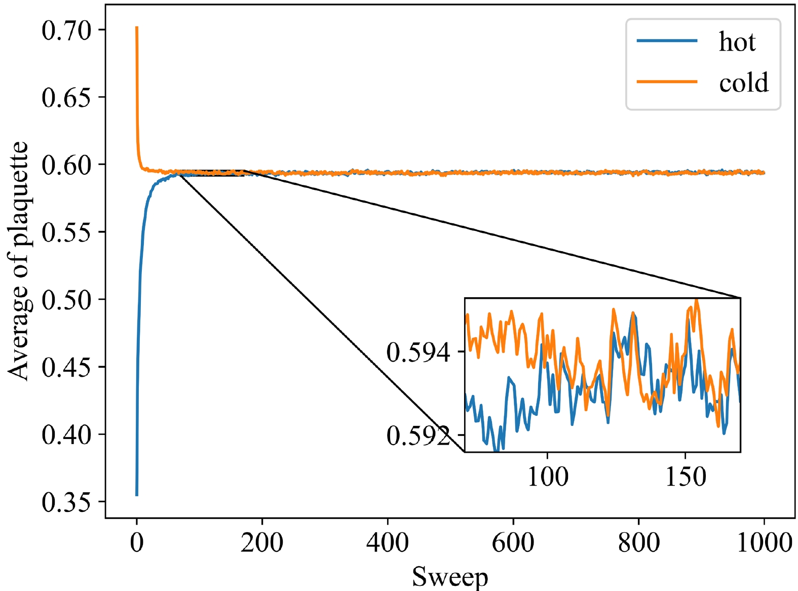
Figure 1. (color online) Evolution of the average of plaquette under different initial conditions.
$ \begin{array}{*{20}{l}} {C_X}\left( {{X_i},{X_{i + t}}} \right) = \langle {{X_i}{X_{i + t}}} \rangle - \langle {{X_i}} \rangle \langle {{X_{i + t}}} \rangle . \end{array} $

(9) We note
$ C_X\left(t\right)\mathrm{=}C_X\left(X_i,\mathrm{\ } X_{i+t}\right) $ at equilibrium and the normalized autocorrelation function$ \Gamma_X\left(t\right)=\frac{C_X\left(t\right)}{C_X\left(0\right)} $ . The integral autocorrelation time is defined as$ \begin{array}{*{20}{l}} {\tau _{X,int}}= \dfrac{1}{2} + {\displaystyle\sum\limits_{t = 1}^N {{\Gamma _X}(t)}} . \end{array} $

(10) We apply the topological charge to calculate the integral autocorrelation time as 0.416, which indicates that each of the data can be regarded as independent because
$N/2\tau_{X,\mathrm{int}} > N$ [8], where a total of 1000 configurations are sampled with intervals of 200 sweeps.In addition, the static QCD potential is used to set the scale and can be parameterized by
$ V\left(r\right)=A+\frac{B}{r}+\sigma r $ [8]. The Sommer parameter$ r_\mathrm{0} $ is defined as$ \begin{array}{*{20}{l}} \left(r^2\dfrac{{\rm d}V\left(r\right)}{{\rm d}r}\right)_{r=r_0}=1.65, \end{array} $

(11) and
$\ r_\mathrm{0}\mathrm{\ =\ }0.49~ {\rm fm}$ is used [27, 28]. The scales are shown in the Table 1.$\rm lattice$ 

β $a/{\rm fm}$ 

$ N_{cnfg} $ 

$ {r_0}/a $ 

$L/{\rm fm}$ 

$ 24\times{12}^3 $ 

6.0 0.093(3) 1000 5.30(15) 1.11(3) Table 1. Setting scales through the static QCD potential.
-
For our purposes, suitable ML models should be constructed to study the characteristics of topological charge and topological charge density. For the large tensor data generated in this study, the DCGAN does not perform well owing to excessive transposed convolution. Therefore, a new frame of the DCGAN is proposed to generate topological charge and topological charge density for our study. Compared with the original DCGAN frame, we construct a new scaling structure. Several fully connected layers are added to our solution such that the layers of transposed convolution can be reduced while processing large tensors. The overall structure of the modified DCGAN (M-DCGAN) is shown in Fig. 2.

Figure 2. (color online) Overall structure of the M-DCGAN.
The structure of the generator for the N-dimensional M-DCGAN (ND M-DCGAN) is explained in Table 2 using the 1D M-DCGAN as an example. For the ND model, the content of each layer must be adjusted according to the dimension. Moreover, the functions of various types of layers are as follows. The fully connected layers and transposed convolution are applied to amplify and reshape the input latent variable with a normal distribution. The convolution is applied to scale down and reshape the previously enlarged data. This new scaling structure is beneficial for large tensor data. Batch normalization is exerted to improve generation. All layers use LeakyReLU activation, except the output layer, which uses Tanh.
$ \rm Layer (type) $ 

$ \rm Output Shape $ 

$ \rm Parameter number $ 

Linear-1 $ [-1, 10000] $ 

1,000,000 BatchNorm1d-2 $ [-1, 10000] $ 

20,000 LeakyReLU-3 $ [-1, 10000] $ 

0 Linear-4 $ [-1, 100] $ 

1,000,000 BatchNorm1d-5 $ [-1, 100] $ 

200 LeakyReLU-6 $ [-1, 100] $ 

0 Linear-7 $ [-1, 4] $ 

400 BatchNorm1d-8 $ [-1, 4] $ 

8 LeakyReLU-9 $ [-1, 4] $ 

0 Linear-10 $ [-1, 100] $ 

400 BatchNorm1d-11 $ [-1, 100] $ 

200 LeakyReLU-12 $ [-1, 100] $ 

0 Linear-13 $ [-1, 4] $ 

400 BatchNorm1d-14 $ [-1, 4] $ 

8 LeakyReLU-15 $ [-1, 4] $ 

0 Linear-16 $ [-1, 100] $ 

400 BatchNorm1d-17 $ [-1, 100] $ 

200 LeakyReLU-18 $ [-1, 100] $ 

0 Linear-19 $ [-1, 6400] $ 

640,000 BatchNorm1d-20 $ [-1, 6400] $ 

12,800 LeakyReLU-21 $ [-1, 6400] $ 

0 ConvTranspose1d-22 $ [-1, 128, 25] $ 

98,304 BatchNorm1d-23 $ [-1, 128, 25] $ 

256 LeakyReLU-24 $ [-1, 128, 25] $ 

0 ConvTranspose1d-25 $ [-1, 64, 50] $ 

32,768 BatchNorm1d-26 $ [-1, 64, 50] $ 

128 LeakyReLU-27 $ [-1, 64, 50] $ 

0 ConvTranspose1d-28 $ [-1, 1, 100] $ 

256 Tanh-29 $ [-1, 1, 100] $ 

0 Table 2. Structure of the generator for the 1D M-DCGAN. Layers 1-21 constitute the new scaling structure.
The input of the generator for the 1D M-DCGAN is a random latent variable tensor with shape [–1, 100], and the output is a tensor with shape [–1, 1, 100], where –1 is an undetermined parameter. For example, we must generate 800 topological charge values, the input shape is [8, 100], and the output shape is [8, 1, 100]. Finally, the output must be reshaped into an 800-dimensional vector. These 800 data can form a distribution.
The structure of the discriminator for the ND M-DCGAN is described in Table 3, taking the 1D M-DCGAN as an example. The convolution is used to scale down and reshape the images. All layers use LeakyReLU, except for the output layer. It is worth noting that the sigmoid layer is placed in the loss function BCEWithLogitsLoss in this study. Dropout is used in the discriminator owing to the small number of training samples for topological charge density. The parameters in Table 3 are explained as follows. The input shape for Conv1d-1 in Table 3 is [–1, 1, 100], the shape of the output is [–1, 64, 50], and the kernel size is 4; therefore, the parameter number is
$ 1 \times 64 \times 4 = 256 $ .$ \rm Layer (type) $ 

$ \rm Output Shape $ 

$ \rm Parameter number $ 

Conv1d-1 $ [-1, 64, 50] $ 

256 LeakyReLU-2 $ [-1, 64, 50] $ 

0 Dropout-3 $ [-1, 64, 50] $ 

0 Conv1d-4 $ [-1, 128, 25] $ 

32,768 LeakyReLU-5 $ [-1, 128, 25] $ 

0 Dropout-6 $ [-1, 128, 25] $ 

0 Linear-7 $ [-1, 1] $ 

3,200 Table 3. Structure of the discriminator for the 1D M-DCGAN.
The optimizer is the Adam, which comprehensively deals with the variable learning rate and momentum proposed by Kingma and Ba [29]. We choose the Adam as a suitable optimizer because it requires less memory, automatically adjusts the learning rate, and limits the update step size to a general range. It is also suitable for large-scale data and parameter scenarios.
As a result, the M-DCGAN models can generate 1D topological charge and 4D topological charge density directly to save computational time after training. The 1D M-DCGAN and 4D M-DCGAN use the same structure described above except for different dimensions and realize unsupervised generation without labels. We adopt the mini-batch method in the training phase. In addition, some programs are based on Pytorch [30].
-
First, we present the distribution of the topological charge simulated by MC with Wilson flow for the cases where the topological charge number is 100 and 300. The right sub-plot of Fig. 3 shows that the fourth root of topological susceptibility is
${\chi_t}^{1/4}=191.8\pm3.9 ~{\rm MeV}$ in terms of$N_{\rm flow}=600$ , and a reference calculation in the literature is${\chi_t}^{1/4}=191\pm 5 ~{\rm MeV}$ [31]. We use the jack-knife to analyze the error of the data [32]. Moreover, the topological charge Q is distributed near integers, as shown in Fig. 3 , which is consistent with the aforementioned conclusion that Q is an integer in the continuum. Furthermore, the topological charge distribution should be symmetric about the origin. However, we can see that the distribution in the left panel of Fig. 3 does not have good symmetry owing to the poor statistics of the data. Therefore, it is better to improve the distribution of data by increasing their statistics. In MC simulations, increasing the amount of data will result in a rapid increase in storage usage and time cost. Fortunately, the ML model can almost avoid this problem. The ML model can immediately generate corresponding data to improve the accuracy of the results once it has finished training. Next, we discuss the details of two methods, MC with Wilson flow and ML with the M-DCGAN scheme, and apply a combination of the two methods to generate the distribution of topological charge more efficiently.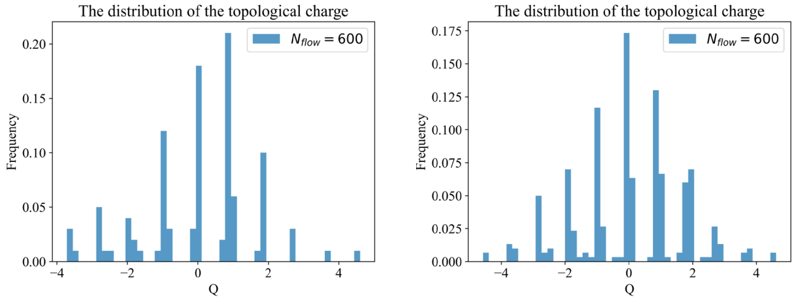
Figure 3. (color online) Distribution of the topological charge based on MC with Wilson flow time steps
$N_{\rm flow}=600$ . The numbers of topological charge are 100 for the left sub-plot and 300 for the right sub-plot.For MC, we simulate 1600 configurations of the lattice gauge field and calculate the topological charge distribution and the fourth root of the topological susceptibility
$ {\chi_t}^{1/4}=190.9\pm1.7~ {\rm MeV} $ from these configurations, with 25 CPU cores in our computations. The details are shown in Table 4.$ \rm Data volume $ 

${\chi_t}^{1/4}({\rm MC})/{\rm MeV}$ 

${\chi_t}^{1/4}({\rm ML})/{\rm MeV}$ 

400 $ 191.2\pm3.5 $ 

$ 191.6\pm3.5 $ 

600 $ 189.4\pm2.9 $ 

$ 191.0\pm2.8 $ 

800 $ 190.6\pm2.4 $ 

$ 191.4\pm2.5 $ 

1000 $ 191.4\pm2.1 $ 

$ 190.6\pm2.2 $ 

1200 $ 191.2\pm2.0 $ 

$ 191.4\pm2.0 $ 

1400 $ 191.6\pm1.8 $ 

$ 191.1\pm1.9 $ 

1600 $ 190.9\pm1.7 $ 

$ 191.1\pm1.7 $ 

Table 4. Fourth root of the topological susceptibility
$ {\chi_t}^{1/4} $ for MC and ML.For ML, we consider applying the 1D M-DCGAN to generate the topological charge used for the original MC data as training data. First, we must determine the suitable data volume of training data. We test the training processes with training data volumes of 80, 160, and 240 by dividing the training data into 2, 2, and 3 groups, respectively, to train the model. The distributions of topological charge generated by the model trained with different amounts of data are shown in Fig. 4. The distribution in the middle subplot is mainly distributed near integers compared with that in the left subplot; however, its peak does not appear at the position of integer zero. Furthermore, the distribution of the right subplot is mainly centered on the integers and is roughly symmetrical about the integer zero. Therefore, we find that the model trains better as the volume of training data increases. From experience, we prefer to use 300 MC data divided equally into three groups for our training scheme.
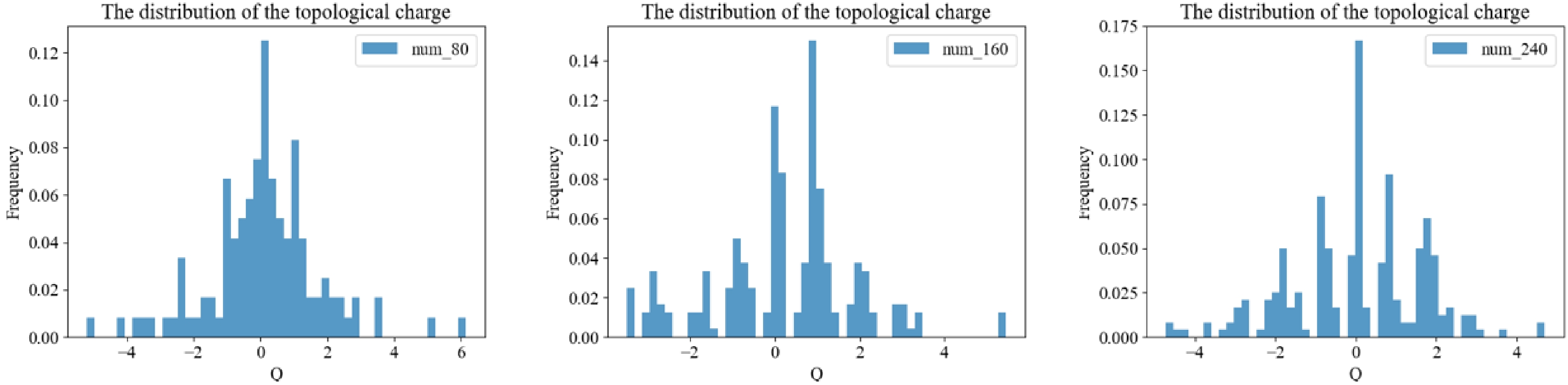
Figure 4. (color online) Comparison of models with 80, 160, and 240 training data.
For our study, the most important aspect to note is the accuracy of the physics results for MC and ML. As shown in Table 4 and Fig. 5 , the data error gradually decreases as the volume of data increases for both MC and ML in which 300 training data are applied to train the 1D M-DCGAN and then 1600 output data are obtained.
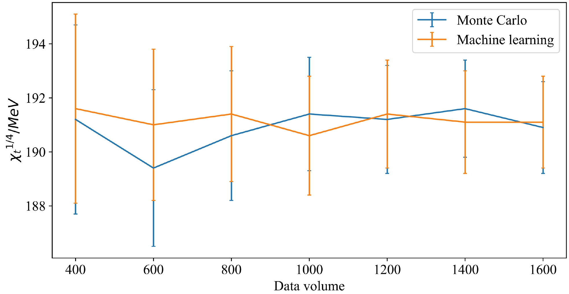
Figure 5. (color online) Fourth root of the topological susceptibility
$ {\chi_t}^{1/4} $ for MC and ML under different data volumes.When we compare the methods of MC and ML, we find that the error of the results from ML is consistent with that by MC. As shown in Table 5, the ML model after training with 300 data can generate the same results as MC, where both the 1600 data numbers are simulated, and the time cost and storage for ML also appear reasonable. Therefore, we can apply the ML scheme to generate suitable data based on the MC simulations to handle the data error and estimate the results efficiently.
$ \rm Method $ 

$ \rm Time/h $ 

$ \rm Storage/MB $ 

${\chi_t}^{1/4}/{\rm MeV}$ 

MC 136 18230 $ 190.9\pm1.7 $ 

ML 26 3429 $ 191.1\pm1.7 $ 

Table 5. Comparison of the MC and ML methods when 1600 data numbers are used. The time and storage of ML data incorporate the effects of a 300 data training process.
Furthermore, the distributions of topological charge for 1600 data generated using the MC and ML methods are shown in Fig. 6. Both distributions exhibit good symmetry, and their data are discretely distributed at integers. These characteristics are consistent with features of the topological charge. In addition, the integrated autocorrelation time of 1600 data for ML is 0.42, which indicates that these data are independent.
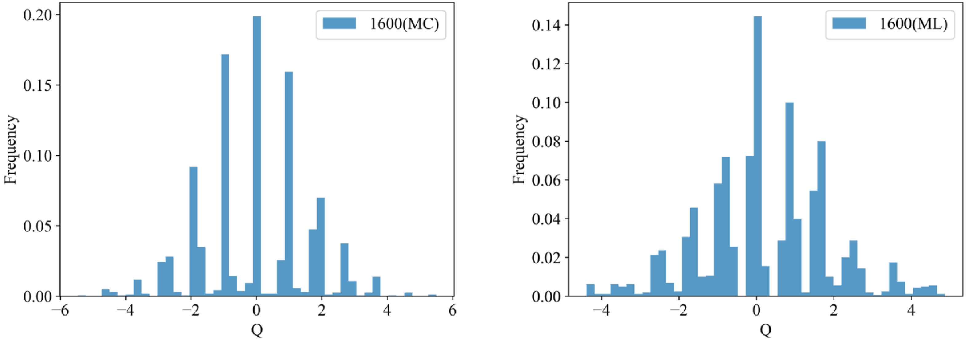
Figure 6. (color online) Distributions of topological charge for MC and ML.
-
Next, the 4D M-DCGAN frame is applied to directly generate the topological charge density in lattice QCD using 300 training data of topological charge density, with
$ N_{\rm flow}=600 $ used to train the model of the 4D M-DCGAN. The input of the generator for the 4D M-DCGAN is a random latent variable tensor with shape [–1, 100], and the output is a tensor with shape [–1, 1, 24, 12, 12, 12]. For example, we generate a topological charge density tensor with the shape [24, 12, 12, 12]. The input shape is [1, 100], and the output shape is [1, 1, 24, 12, 12, 12]. Finally, the output must be reshaped into the tensor with shape [24, 12, 12, 12]. The visualization is referenced from the paper [33] and PyVista [34]. The complete topological charge density is four-dimensional, with a one-dimensional temporal component and three spatial components. From the previous definition of the topological charge density, the topological charge density changes continuously in the time direction in the continuous case. Therefore, the topological charge density changes approximately continuously in the time direction in lattice QCD when the lattice spacing is small. The images of topological charge density simulated using the pseudo heat bath algorithm and Wilson flow is shown in Fig. 7.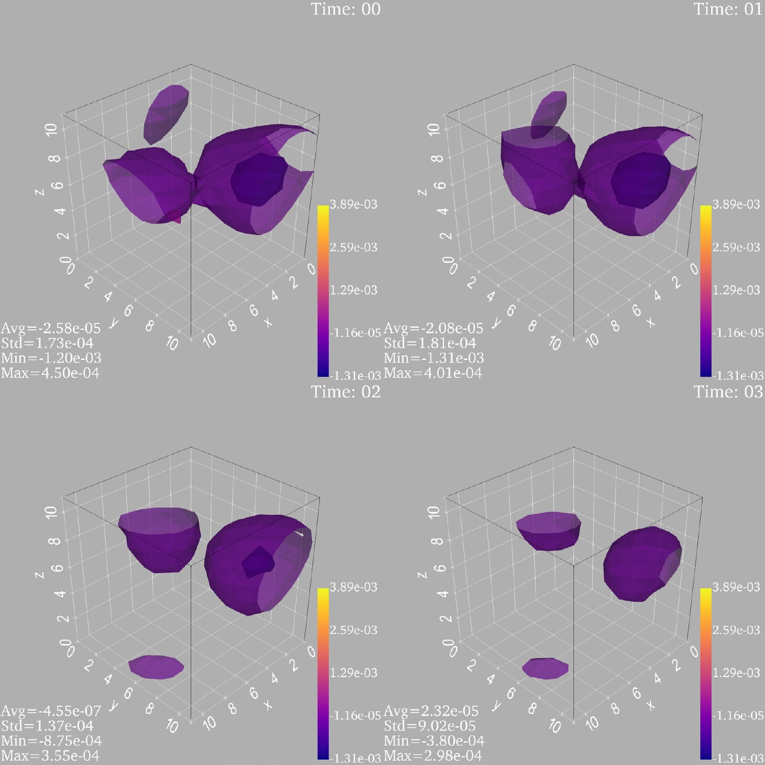
Figure 7. (color online) Images of topological charge density simulated by MC. The four sub-panels correspond to four time slides.
The images of the topological charge density generated by the generator under different epochs are shown in Fig. 8. The 4D M-DCGAN gradually generates clear images from messy images, which indicates that the 4D M-DCGAN does not capture image segments of training data to stitch the images.
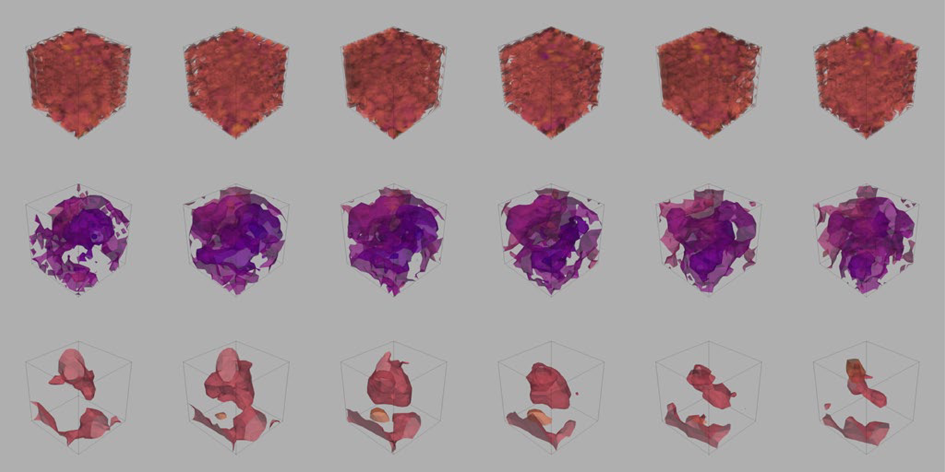
Figure 8. (color online) Sub-images, from top to bottom, are the topological charge density images generated by the generator when the epoch is 100, 200, and 400, and the sub-images of each row are images of the first 6 time slices of topological charge density. Numerical values are omitted for clarity and discussed later.
Furthermore, the quality of the generated 4D image requires an evaluation process. An image produced by the generator is passed to the discriminator for scoring. The discriminator has various evaluation indicators and obtains a set of values. These values are then calculated using a certain formula to obtain the final score of the image. The program is as follows. The generator inputs the generated data into the well-trained discriminator, and the discriminator outputs a vector with various indicators. Then, this vector is input into BCEWithLogitsLoss to generate an evaluation value. It is worth noting that a smaller evaluation value suggests a higher quality of the generated image. We then convert the evaluation value to a score between zero and one hundred. We introduce the following formula to calculate this score:
$ \begin{array}{*{20}{l}} {\rm score} = 100 \times \dfrac{{{\rm ln}{{\bar l}_r} - {\rm ln}\left( {1 + {l_g}} \right)}}{{{\rm ln}{{\bar l}_r}}} = 100 \times \dfrac{{{{{\rm ln}}}[{{\bar l}_r}/\left( {1 + {l_g}} \right)]}}{{{\rm ln}{{\bar l}_r}}}, \end{array} $

(12) where
$ {\bar{l}}_r $ is the average of the evaluation values of 300 random tensors with a size of$ Nt\times Nx\times Ny\times Nz $ under the discriminator and BCEWithLogitsLoss, and$ l_g $ is the evaluation value of a tensor with the same size as the topological charge density generated using a certain method. Logarithms are used in the formula because$ {\bar{l}}_r $ reaches the order of millions. We must use logarithms to reduce the difference between$ l_g $ and$ {\bar{l}}_r $ , otherwise the real data score will be concentrated between 99 and 100.${\rm ln}\left(1+l_g\right)$ is used to ensure that the score is 100 when$ l_g $ is zero. In addition, the criteria for using the score to judge the quality of the data is given later in conjunction with the discriminator.As discussed above, the construction method for the score requires a well-trained discriminator. Therefore, a well-trained discriminator must be selected. The loss of the discriminator is shown in Fig. 9. The smaller the loss, the stronger the discrimination ability of the discriminator. The loss of the discriminator is not only small but also does not change considerably after 6000 epochs. Therefore, a well-trained discriminator can be selected after 6000 epochs. Furthermore, we must determine the score standard of the generated data after selecting the discriminator. We select another 300 topological charge density data calculated by MC as the testing data and then input the training, testing, and random data into the discriminator to obtain the score according to the method mentioned above. The result is shown in Fig. 10. As shown, the discriminator distinguishes topological charge density data from random data, and the scores of the real data, which include the training and testing data, are in the range of 80 to 100; hence, the generated data will be sufficiently credible if the score is also in this range.
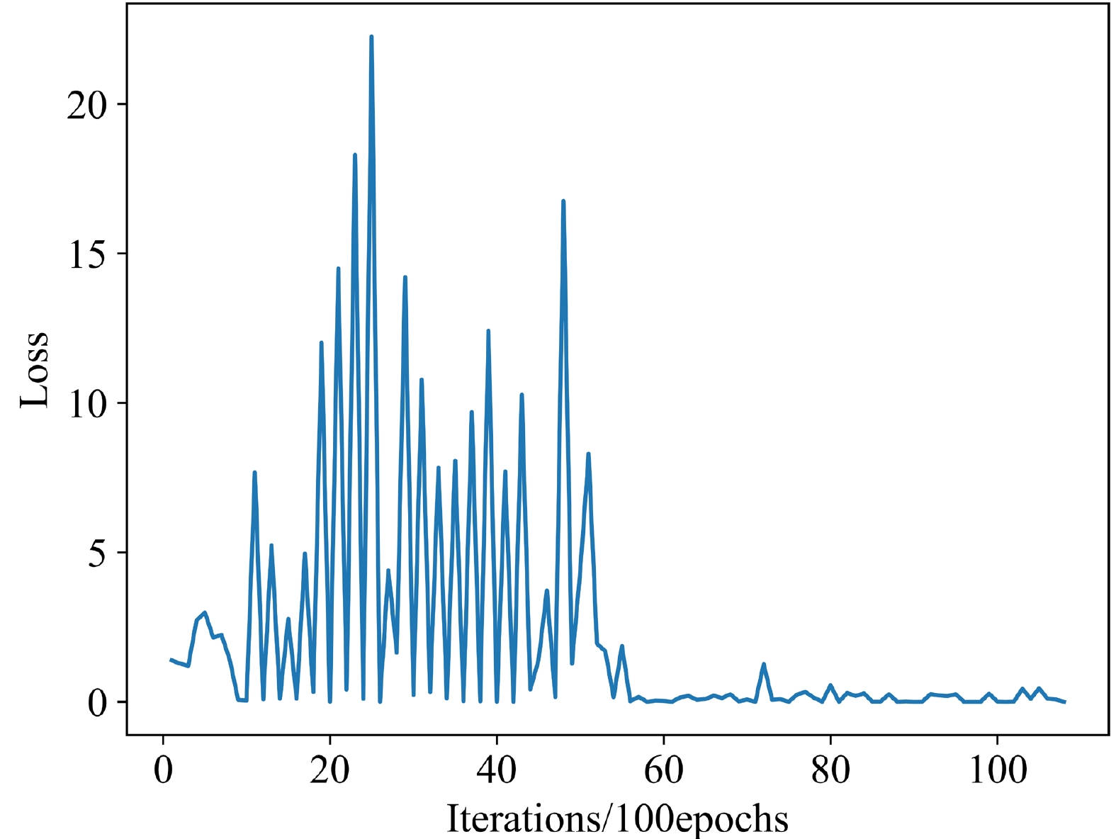
Figure 9. (color online) Losses of the discriminator in different training epochs.

Figure 10. (color online) Scores obtained by the training, testing, and random data.
Several images of topological charge density with different topological charges generated by the 4D M-DCGAN are shown in Fig. 11, and the scores of these topological charge density data are shown in Table 6. These scores are all greater than 80, which indicates that the generated 4D images are of high quality, or the generated data of the topological charge density are consistent with the original training data. As shown in Figs. 10 and 11, the 4D M-DCGAN not only generates images of topological charge density with good shape, similar to the real data in Fig. 7, but also has a good performance in terms of the continuity of topological charge density in the time direction and the value of topological charge.
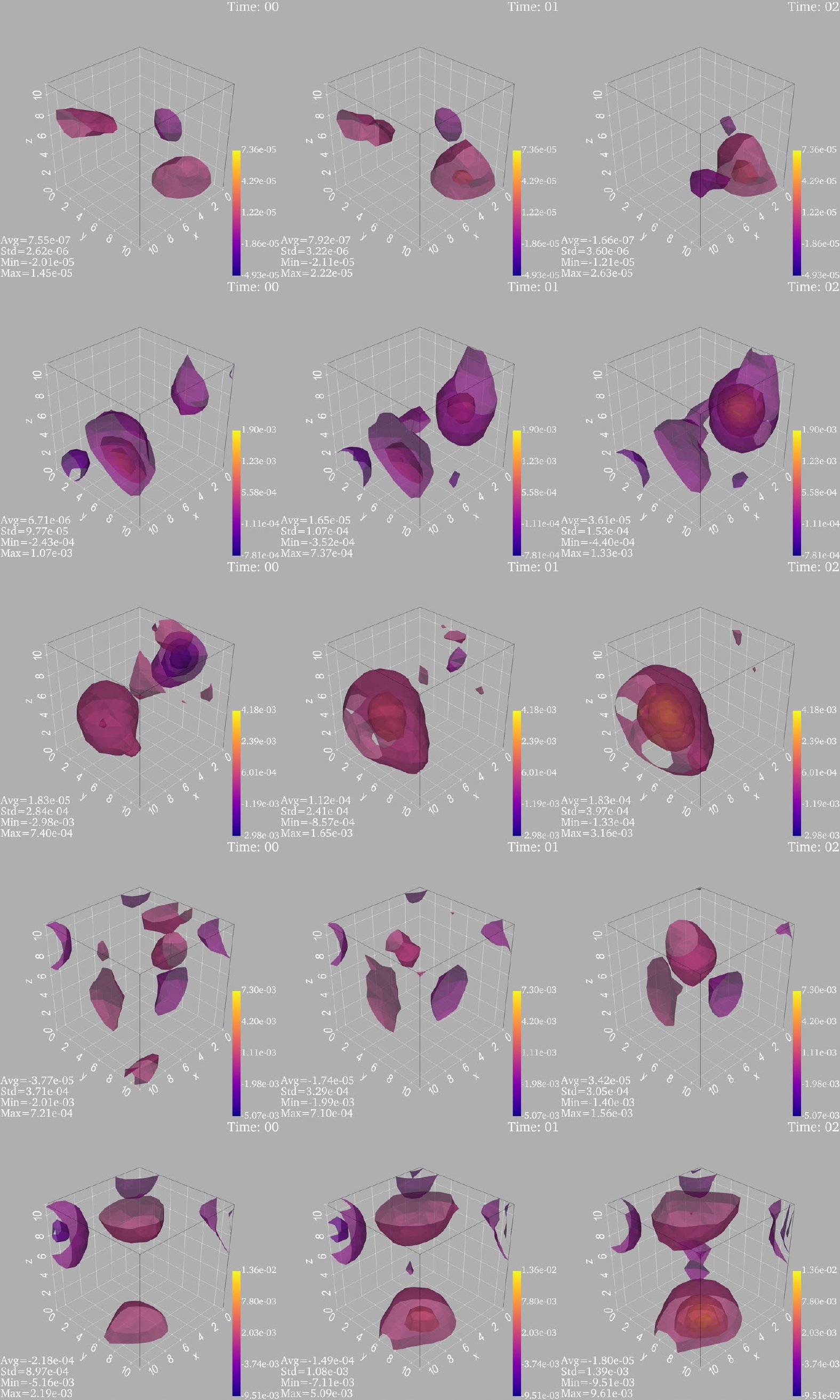
Figure 11. (color online) Images of topological charge density for different values of topological charge. Each row shows the first three sub-images of a topological charge density in the time direction. The sub-images from top to bottom correspond to topological charges of 0.02, 1.15, 2.33, 2.98, and 3.84, respectively.
$\rm topological\;\; charge$ 

0.02 1.15 2.33 2.98 3.84 $ \rm score $ 

96 100 95 100 87 Table 6. Scores of topological charge density with different topological charges under a well-trained discriminator and BCEWithLogitsLoss.
-
In this study, the topological quantities of lattice QCD are investigated by a MC simulation combined with the M-DCGAN frame. We then apply a 1D M-DCGAN to generate the distribution of topological charge and a 4D M-DCGAN to calculate the data of topological charge density to show the potential for the application of the ML technique in lattice QCD. Our conclusions are as follows.
First, compared with MC with Wilson flow, the ML technique with our 1D M-DCGAN scheme reveals its efficiency for MC simulations. The data generated by the 1D M-DCGAN trained with three sets of 100 data are more accurate than the corresponding data from the MC simulation in terms of the topological susceptibility.
Second, from different training epochs, we find that the 4D M-DCGAN gradually generates clear images from messy images step by step instead of simply capturing image segments of training data to stitch the images. Furthermore, the quality of the images of topological charge density from the 4D M-DCGAN generator is generally high through the evaluation of a well-trained discriminator and BCEWithLogitsLoss. More importantly, the 4D M-DCGAN not only generates images of topological charge density with a good shape consistent with that of the image obtained by MC, but also has a good performance in terms of the continuity of topological charge density in the time direction and the values of topological charge centered around integers.
Finally, we hope that the M-DCGAN scheme can be applied to study other physics problems in lattice QCD and help simulate interesting quantities more efficiently.
-
This study was conducted based on the Chroma applied to simulate the configuration of the lattice gauge field. We are grateful to the relevant contributors to the Chroma.
Study of the topological quantities of lattice QCD using a modified DCGAN frame
- Received Date: 2024-02-20
- Available Online: 2024-05-15
Abstract: A modified deep convolutional generative adversarial network (M-DCGAN) frame is proposed to study the N-dimensional (ND) topological quantities in lattice QCD based on Monte Carlo (MC) simulations. We construct a new scaling structure including fully connected layers to support the generation of high-quality high-dimensional images for the M-DCGAN. Our results suggest that the M-DCGAN scheme of machine learning will help to more efficiently calculate the 1D distribution of topological charge and the 4D topological charge density compared with MC simulation alone.


 DownLoad: