


 Abstract
 HTML
HTML Reference
 Related
 PDF
PDF


-
Unveiling the proton structure is a long-standing interest in high energy physics. Currently, we are still far from comprehensively understanding the spatial structure of the proton, including the event-by-event fluctuating shape and the profile density of its valence quarks. Experimentally, deeply inelastic electron-proton scattering (DIS) is a good candidate for resolving the internal structure of the proton, where a virtual photon emitted from the electron is used as a probe to explore the proton. Based on the inclusive DIS, the H1 and ZEUS collaborations at HERA measured the proton structure functions and obtained parton distribution functions [1, 2]. Diffractive DIS (DDIS) of the
$ \gamma^*+p $ interaction is an especially effective approach to studying the internal proton structure because there is a large rapidity gap between the produced particle and scattered proton owing to the color singlet exchange in the DDIS process [3−5]. This typical signature can be exploited to identify diffractive events, which can provide the cleanest data for the observables, e.g., the differential cross-section${\rm d}\sigma^{\gamma^*+p}/{\rm d}t$ and diffractive slope$ B_D $ . Moreover, future diffractive electron-ion collisions at the Electron-Ion Collider (EIC) [6], Large Hadron Electron Collider (LHeC) [7], and Electron-ion Collider in China (EicC) [8] will provide more accurate data and further enter the small-x dynamic regions, which will provide an unprecedented chance to access the detailed structure of the proton.Theoretically, color glass condensate (CGC) effective field theory is a powerful tool in describing the inclusive
$ \gamma^*+p $ DIS process [9−17] and proton geometric shape [4, 5, 18], in which the scattering process can be viewed as a virtual photon fluctuating into a quark-antiquark dipole, followed by the dipole interacting with the proton target. Thus, the total cross-section can be simply factorized into the virtual photon wavefunction multiplying the dipole scattering cross-section. The CGC description of the DIS process has two significant aspects. First, it improves our understanding of the$ \gamma^*+p $ interaction. In CGC framework, all information about the QCD dynamics of the interactions is included in the dipole-proton amplitude. Second, it dramatically simplifies the total cross-section calculations because the virtual photon wavefunction can be precisely computed by QED, and the dipole cross-section can be obtained by solving the Balitsky-Kovchegov (BK) [19, 20] or JIMWLK equation [19, 21−24]. Furthermore, the CGC framework can be extended to describe$ \gamma^*+p $ DDIS where the target proton remains intact after scattering of the virtual photon [25−27].It is known that DDIS is a useful probe for investigating the proton shape at high energies. At high energies, the DDIS process is driven by the gluon content of the target, which renders the cross-section of the DDIS process proportional to the square of the dipole amplitude. Therefore, the cross-section is highly sensitive to the underlying QCD dynamics compared to that in the inclusive DIS. Moreover, the differential cross-section of DDIS (
${\rm d}\sigma/{\rm d}t$ ) offers the possibility of obtaining the transverse spatial distributions of partons in the proton, as the squared four-momentum transfer (t) is the Fourier conjugate of the impact parameter profile of the proton. As a consequence, DDIS can provide access to investigate the geometric structure of the proton.In the past decade, the DDIS process has been widely used to study the proton shape [4, 5, 28−34]. Based on the constituent quark picture of the proton, several hot spot models have been proposed to describe the proton shape in the exclusive DDIS [5, 31, 32, 35], where the hot spot is actually a gluon formed by the emission from a large x valence quark. At high energy, it has been found that the proton is not a spherical object; it consists of several hot spots and its shape fluctuates event-by-event [3]. The hot spot models can give a good description of the vector meson productions at HERA. However, all the hot spot models simply assume that the valence quarks (up and down quarks) have the same profile densities, namely, they obey the Gaussian distribution with the same width (
${B_u=B_d}$ ). In fact, the gluon distribution of each valence quark can be different in event-by-event experiments. Recently, a lattice QCD study of the proton generalized parton distributions (GPDs) in Ref. [36] showed that the up quark exhibits a different distribution width from the down quark in the unpolarized proton, and the distortions between the up and down quarks are also different in the polarized proton. Their findings inspire us to study the profile density of the valence quark of the proton.In our previous study [37], we extended the hot spot model to a refined hot spot model and used the exclusive vector meson production to study the individual width of the proton. We obtained a very interesting result: the width of the valence up quark of the proton was larger than or equal to the width of the down quark (
$ {B_u\geq B_d} $ ), which is favored by the HERA measurements. In this study, we focus on the deeply virtual Compton scattering (DVCS) process, which is one type of exclusive diffractive deep inelastic scattering process. One of the motivations behind this study is that although the DVCS cross-sections are smaller than those of vector meson productions, they are not impacted by the theoretical uncertainties associated with the scarce knowledge of the vector meson wavefunction because the real photon wavefunction can be precisely calculated by QED, whereas the vector meson wavefunctions can only be modeled with relatively large model parameters. Thus, the DVCS process can be used as a highly accurate and direct probe to study the spatial structure of the proton. Another motivation is associated with the expectation that the DVCS process could be used to study the collision energy impact on the width of the individual valence quark and improve our understanding of the 3-dimensional imaging of the valence quark inside the proton at high energy. We find that the discrepancies, which reflect the difference in the distribution width of the valence quark, are broadened as the collision energy increases. As shown in Sec. IV, the discrepancies become larger at LHeC than at HERA and EIC energies. We also find that in the DVCS process, the discrepancies shift to a smaller momentum transfer region (t:$ 0.2\sim1\; \mathrm{GeV^{2}} $ ) than that of the exclusive diffractive vector meson production process, which was studied in Ref. [37], where remarkable discrepancies are found in the relatively large t region. The smaller t means that higher statistical experimental data can be obtained, which can provide more tight constraints on the width parameters. -
In this section, we provide a brief overview of the formalism used to calculate the differential cross-section of DVCS in electron-proton collisions. We study the DVCS process based on the Good-Walker picture and CGC framework. In the Good-Walker picture, the DDIS process can be classified into two types, coherent and incoherent diffraction, in terms of the scattered target proton dissociation. For coherent diffraction, the proton remains intact after scattering, and the differential cross-section is given by [38]
$ \frac{{\rm d}\sigma^{\gamma^*p\rightarrow Vp}}{{\rm d}t} = \frac{(1+\beta^2)R_g^2}{16\pi}\Big|\big\langle \mathcal{A}^{\gamma^*p\rightarrow Vp}(x,Q^2,{\bf{\Delta}})\big\rangle\Big|^2, $

(1) where
$ \langle\cdots\rangle $ represents the average over the configurations of the proton wavefunction.$ \mathcal{A}^{\gamma^*p\rightarrow Vp} $ is the diffractive scattering amplitude, detailed information on which is introduced later.$ 1+\beta^2 $ and$ R_g $ in Eq. (1) are the corrections from the real part of$ \mathcal{A}^{\gamma^*p\rightarrow Vp} $ and skewness, respectively, where β is the ratio of the real to imaginary part of the scattering amplitude, which is written as [38]$ \beta = \tan\Big(\frac{\pi\delta}{2}\Big) $

(2) with
$ \delta = \frac{\partial\ln\big(\mathcal{A}_{T,L}^{\gamma^*p\rightarrow Vp}\big)}{\partial\ln(1/x)}. $

(3) We take
$ R_g $ from Ref. [38] as$ R_g =\frac{2^{2\delta+3}}{\sqrt{\pi}}\frac{\Gamma(\delta+5/2)}{\Gamma(\delta+4)}. $

(4) In incoherent diffraction, the proton is dissociated after scattering, and the differential cross-section is proportional to the variance of the proton profile [39, 40],
$ \begin{aligned}[b] \frac{{\rm d}\sigma^{\gamma^*p\rightarrow Vp}}{{\rm d}t} =\;& \frac{(1+\beta^2)R_g^2}{16\pi}\Bigg(\Big\langle\big|\mathcal{A}^{\gamma^*p\rightarrow Vp}(x,Q^2,{\bf{\Delta}})\big|^2\Big\rangle\\&-\Big|\big\langle \mathcal{A}^{\gamma^*p\rightarrow Vp}(x,Q^2,{\bf{\Delta}})\big\rangle\Big|^2\Bigg), \end{aligned} $

(5) where based on the definition of variance, the first term on the right hand side indicates that the square of the scattering amplitude is performed before obtaining the average over the configurations of the proton wavefunction, and the second term on the right hand side implies that the average of the scattering amplitude over the configurations of the proton wavefunction is performed before obtaining the square of the amplitude. By comparing Eqs. (1) and (5), we can see that the coherent cross-section is calculated using the average over the scattering amplitude; hence, it is only sensitive to the average configuration of the proton and provides overall information about the structure of the proton (not the detailed structure). Conversely, the incoherent cross-section is computed using the variance of the proton, which renders the incoherent cross-section extremely sensitive to the details of the structural fluctuations of the proton. Therefore, the incoherent diffractive cross-section can provide excellent access to explore the internal structure of the proton.
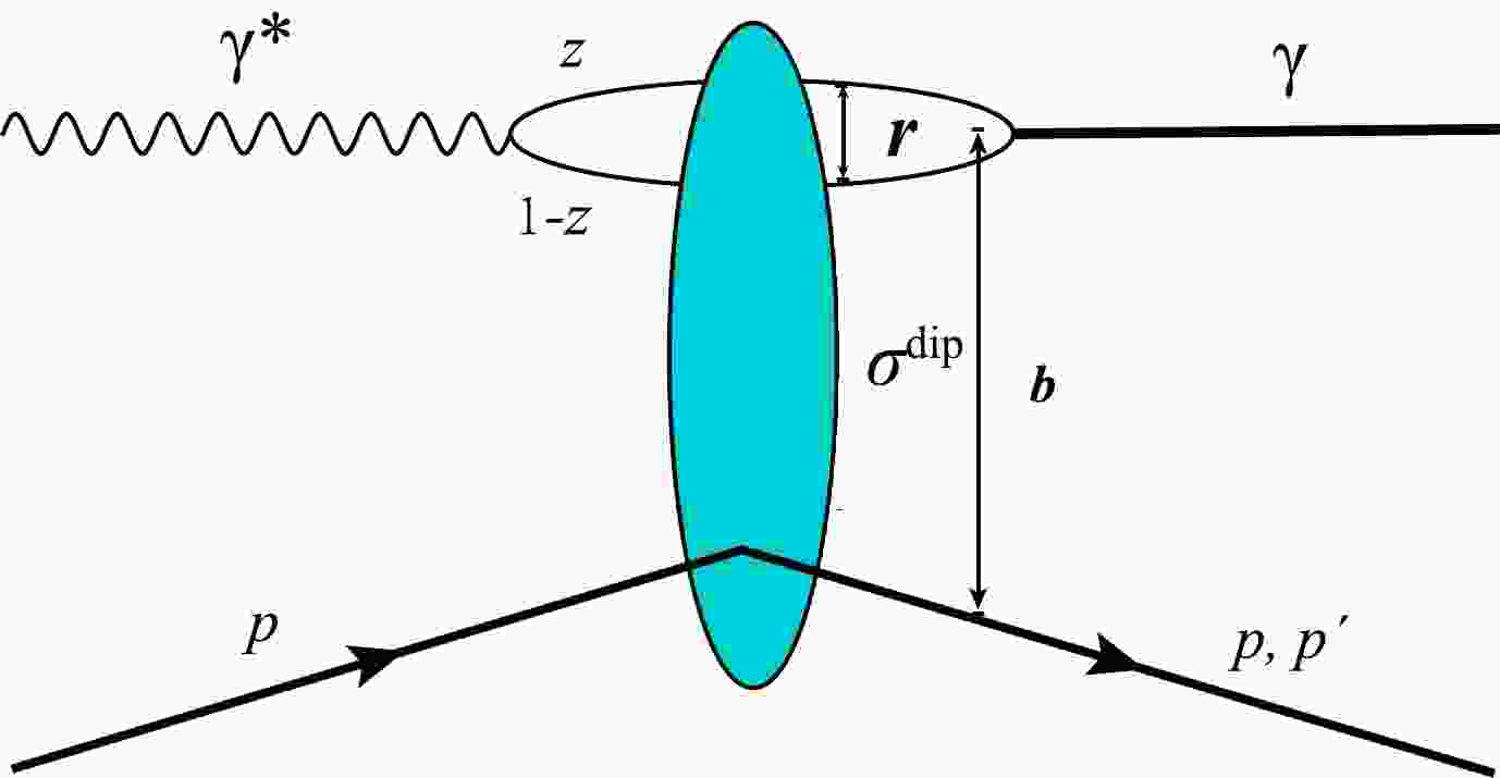
Let us now introduce the diffractive scattering amplitude. Based on the CGC framework and color dipole picture, the DVCS process (
$ \gamma^*+p\rightarrow \gamma + p $ ) can be divided into three sub-processes, as shown in Fig. 1. (1) The virtual photon fluctuates into a quark-antiquark dipole, (2) the dipole interacts with the proton target, and (3) the dipole recombines into a real photon. Here, the outgoing photon is real, and thus the DVCS process can be directly observed in DIS experiments. The scattering amplitude of DVCS can be obtained via the convolution of the overlap function and dipole cross-section [38],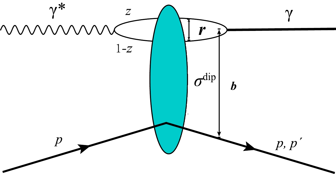
Figure 1. (color online) Deeply virtual Compton scattering process in the dipole picture.
$ \begin{aligned}[b] \mathcal{A}^{\gamma^*p\rightarrow Vp}_{T,L}(x, Q^2, {\bf{\Delta}}) = \;&{\rm i} \int {\rm d}^2{\boldsymbol{r}}\int {\rm d}^2{\boldsymbol{b}}\int\frac{{\rm d}z}{4\pi}\big(\Psi_{\gamma^*}^*\Psi_\gamma\big)^f\\&\exp\Big\{-{\rm d}\big[{\boldsymbol{b}}-(1-z){\boldsymbol{r}}\big]\cdot{\bf{\Delta}}\Big\} \frac{{\rm d}\sigma^{\mathrm{dip}}}{{\rm d}^2{\boldsymbol{b}}}, \end{aligned} $

(6) where
$ {\boldsymbol{r}} $ denotes the transverse size of the quark-antiquark dipole,$ {\boldsymbol{b}} $ represents the impact parameter of the dipole with respect to the proton target,$ {\boldsymbol{b}}-(1-z){\boldsymbol{r}} $ is the Fourier conjugate to the momentum transfer$ {\bf{\Delta}} $ ($ {\bf{\Delta}}^2=-t $ ), z and$ 1-z $ refer to the longitudinal momentum fraction of the quark and antiquark, respectively, and$ Q^2 $ is the virtuality of the photon. The overlap function in Eq. (6) is given by [38]$ \begin{aligned}[b] \big(\Psi_{\gamma^*}^*\Psi_\gamma\big)^f=\;&\frac{N_c\alpha_{\rm em}}{2\pi^2}e_f^2\Big\{[z^2+(1-z)^2]\epsilon_1K_1(\epsilon r)m_fK_1(m_f r)\\&+m_f^2K_0(\epsilon r)K_0(m_f r)\Big\}, \end{aligned} $

(7) where
$ e_f $ and$ m_f $ are the charge and mass of a quark with flavor f, respectively,$ K_0 $ and$ K_1 $ are the modified Bessel functions of the second type,$ \epsilon^2\equiv z(1-z)Q^2+m_f^2 $ , and$ N_c=3 $ is the number of colors. We would like to note that we investigated the proton shape with exclusive diffractive vector meson production in Ref. [37] . Where the wavefunctions of the vector meson could not be directly calculated, the modelling wavefunctions were used to study the individual quark width; thus, the final results inevitably included uncertainties from the modeling. In this study, the wavefunction in Eq. (7), which can be precisely calculated by QED, is used to estimate the DVCS differential cross-section, as shown in the next section; therefore, uncertainties from the modeling of the wavefunction are effectively avoided.The dipole-proton cross-section is a key ingredient in Eq. (6) because it includes all the QCD information on the DVCS process. According to the optical theorem, the dipole-proton cross-section can be calculated using the forward dipole scattering amplitude,
$ \frac{{\rm d}\sigma^{\mathrm{dip}}}{{\rm d}^2{\boldsymbol{b}}}({\boldsymbol{b}}, {\boldsymbol{r}}, x) = 2N({\boldsymbol{b}}, {\boldsymbol{r}}, x), $

(8) where N is the dipole amplitude whose rapidity (or energy) evolution is characterized by the non-linear evolution equation, e.g., the BK or JIMWLK equation. In the past two decades, there has been significant progress in understanding the non-linear evolution of QCD in terms of the CGC. The LO BK equation was successfully extended to the NLO case [41−44], and the BK equation was solved analytically [45−48] and numerically [49, 50]. Although the analytic dipole amplitude is obtained, it only works in the saturation region, and the impact parameter dependence of the numerical dipole amplitude exhibits a strong Coulomb tail. However, the impact parameter dependence of the dipole amplitude is a key factor when studying the proton shape. In spite of the reason mentioned above, we choose the impact parameter dependent saturation model (IPsat) [51] to obtain the dipole amplitude in this study, which is widely used in the literature and has been very successfully used to describe data at HERA, RHIC, and LHC energies. Therefore, the dipole cross-section can be expressed as
$ \begin{aligned}[b] \frac{{\rm d}\sigma^{\mathrm{dip}}}{{\rm d}^2{\boldsymbol{b}}}({\boldsymbol{b}}, {\boldsymbol{r}}, x) =\;& 2N({\boldsymbol{b}}, {\boldsymbol{r}}, x) \\ =\;& 2\bigg[1-\exp\Big(-\frac{\pi^2{\boldsymbol{r}}^2}{2N_c}\alpha_s(\mu^2)xg(x,\mu^2)T_p({\boldsymbol{b}})\Big)\bigg], \end{aligned} $

(9) where
$ T_p({\boldsymbol{b}}) $ is the profile function of the proton, which is assumed to be Gaussian [4, 5],$ T_{p}({\boldsymbol{b}})=\frac{1}{2\pi {B_p}}\exp\bigg(-\frac{{\boldsymbol{b}}^2}{2 {B_p}}\bigg), $

(10) where
$ {B_p} $ is the proton width. In Eq. (9),$ xg(x,\mu^2) $ is the gluon density, whose evolution obeys the DGLAP evolution equation. μ in Eq. (9) is a scale that relates to$ {\boldsymbol{r}} $ as$ \mu^2 = \frac{4}{{\boldsymbol{r}}^2} + \mu_0^2, $

(11) and the initial
$ xg(x,\mu^2) $ at$ \mu_0^2 $ is$ \begin{array}{*{20}{l}} xg(x,\mu_0^2) = A_g x^{-\lambda_g}(1-x)^{5.6}, \end{array} $

(12) where the model parameters
$ \mu_0 $ ,$ A_g $ , and$ \lambda_g $ are taken from Ref. [52].Note that the profile function of the proton in Eq. (9) is for a single event. It does not consider the fluctuation of the proton shape. In fact, the proton shape fluctuates event-by-event. Consequently, the fluctuation has a large impact on the dipole cross-section, which leads to an enhancement in the incoherent
$ J/\psi $ production cross-section [5]. The relevant fluctuations are discussed in the next section. -
There are two important fluctuations playing key roles in the DDIS process: saturation scale and geometric shape fluctuations. First, we introduce the saturation scale fluctuation. It has been shown that this fluctuation is significant in the description of
$ J/\psi $ production data in low t regions at HERA [4, 5]. We consider the saturation scale fluctuations used by Ref. [5], where the saturation scale satisfies a log-normal distribution,$ P\big(\ln Q_s^2/\langle Q_s^2\rangle\big)=\frac{1}{\sqrt{2\pi}\sigma}\exp\Bigg[-\frac{\ln^2Q_s^2/\langle Q_s^2\rangle}{2\sigma^2}\Bigg]. $

(13) In terms of the above distribution, the expectation of
$ Q_s^2/\langle Q_s^2\rangle $ is$ \begin{array}{*{20}{l}} E\big[Q_s^2/\langle Q_s^2\rangle\big]=\exp\big[\sigma^2/2\big]. \end{array} $

(14) We can simply calculate the average of
$ Q_s^2 $ , which is approximately$ 13\% $ (for$ \sigma=0.5 $ ) larger than that without considering the saturation scale fluctuations. Therefore, the log-normal distribution must be normalized to maintain the desired expectation. Note that a recent study demonstrated that saturation scale fluctuations can be interpreted as fluctuations in dipole size [35].The geometric shape of a proton fluctuates event-by-event at high energies. One natural and easy method of investigating proton shape fluctuations is the hot spot model, which assumes that the proton consists of several "gluon clouds" [3−5]. The "gluon cloud" is formed by the gluon emission from the large-x valence quark. It is known that the gluon emission can also differ event-by-event. As a consequence, the proton shape fluctuates event-by-event.
In the hot spot model, the transverse position (
$ {\boldsymbol{b_i}} $ ) and density profile of each constituent quark are both assumed to have Gaussian distributions with width$ { {B_{qp}}} $ and$ {B_{cq}} $ , respectively (where the subscripts$ {qp} $ and$ {cq} $ denote the quark position and constituent quark, respectively). Specifically, the density profile of each constituent quark is expressed as$ T_{{cq}}({\boldsymbol{b}}) = \frac{1}{2\pi {B_{cq}}}\exp\bigg(-\frac{{\boldsymbol{b}}^2}{2{{B_{cq}}}}\bigg). $

(15) Considering the fluctuations, the proton density profile in Eq. (9) should be replaced by [4, 5]
$ T_p({\boldsymbol{b}}) = \frac{1}{N_{hs}}\sum\limits_{i=1}^{N_{hs}}T_{{cq}}\big({\boldsymbol{b}}-{\boldsymbol{b_i}}\big), $

(16) where
$ N_{hs} $ is the number of hot spots.We would like to emphasize that all hot spot models assume that the valence up and down quarks have the same width (
$ {B_u}= {B_d} $ ) in the literature [4, 5, 28−34] but not in our work in Ref. [37]. Thus, the differences between the density profile of the up and down quarks were neglected in Refs. [4, 5, 28−34]. However, a lattice study of the proton's GPDs in Ref. [36] showed that the density profile of the up quark is different from that of the down quark owing to different distortion forces experienced by the up and down quarks, which inspires us to treat$ {B_u} $ and$ {B_d} $ separately.In our previous study [37], we used the vector meson production process to probe
$ {B_u} $ and$ {B_d} $ and found that$ {B_u} \geq {B_d} $ is favored by the HERA data, whereas$ {B_u} < {B_d} $ cannot well reproduce the HERA data. In this study, we use the DVCS process to probe the proton shape for two main reasons. (1) In the DVCS process, the overlap function between the virtual and real photon can be precisely calculated by QED, which significantly reduces the uncertainties from modeling the vector meson wavefunction; thus, the DVCS process can be direct used to probe the spatial structure of the proton. (2) Compared to the vector meson production process, the discrepancies used to distinguish$ {B_u} $ from$ {B_d} $ in the DVCS process are shifted to relative smaller t regions, where a large amount of highly precise experimental data are located, which can help reduce statistical errors in the analysis. -
In this section, we present the numerical results of the coherent and incoherent differential cross-sections of the DVCS processes at HERA, EIC, and LHeC energies. The differential cross-sections are calculated in the cases of
$ {B_u} \geq {B_d} $ and$ {B_u} < {B_d} $ . The results presented below are obtained for 10000 configurations of the proton. -
The DVCS process is a good probe to directly resolve the structure of the proton because the overlap function between the virtual and real photon can be precisely calculated. In this subsection, we study the widths of the up and down quarks using our refined hot spot model [37], where the width of the valence quark is treated separately instead of using a same width for up and down quarks as done in the literature [4, 5, 29−34]. To explore the detailed structure of the proton valence quark, we vary the width parameters
$ {B_u} $ and$ {B_d} $ but keep the average width of the valence quark$ {\bar{B}_{cq}}=(2 {B_u}+ {B_d})/3=1.0 $ unchanged. Note that the 2 in front of$ {B_u} $ represents the two up quarks in a proton. We compare our numerical results with the measurements from the H1 collaboration at HERA at${W}=85\; \mathrm{GeV}$ [53, 54], which corresponds to$ x\sim10^{-3} $ , where our CGC framework is valid.The coherent and incoherent differential cross-sections of the DVCS process as functions of momentum transfer t at
${W}=85\; \mathrm{GeV}$ are shown in Fig. 2. The upper panel of Fig. 2 shows the results calculated at$ Q^2= 8\; \mathrm{GeV^2} $ , whereas the lower panel shows the calculations at$ Q^2=25 \mathrm{GeV^2} $ . The solid curves denote the numerical results of the coherent differential cross-section, and the dashed curves represent the incoherent differential cross-section (similarly defined in subsequent figures). Note that the red curves are calculated using the parameters from the original hot spot model with$ {B_{qp}}=3.0\; \mathrm{GeV^{-2}} $ and$ {\bar{B}_{cq}}=1.0\; \mathrm{GeV^{-2}} $ [4, 5], which can provide a reasonable description of the vector meson production data at HERA. We would like to note that$ {\bar{B}_{cq}} $ is the average width of the valence up and down quarks. The authors in Refs. [4, 5] did not distinguish between the density profiles of up and down quarks. As mentioned above, we maintain$ {\bar{B}_{cq}}=1.0\; \mathrm{GeV^{-2}} $ and select several typical cases ($ {B_u} \geq {B_d} $ and$ {B_u} < {B_d} $ ), e.g.,$ {B_u}=2 {B_d} $ ,$ {B_u}=6 {B_d} $ (left hand panel of Fig. 2) and$ {B_u}= {B_d}/2 $ ,$ {B_u}= {B_d}/6 $ (right hand panel of Fig. 2). Note that the proton shape fluctuates event-by-event, leading to fluctuations in the widths of the up and down quarks event-by-event. As shown in Fig. 2, all of our calculations of coherent differential cross-sections can reproduce the H1 measurements regardless of$ {B_u} \geq {B_d} $ or$ {B_u} < {B_d} $ , because the coherent cross-section is obtained by obtaining the average on the level of the scattering amplitude. Thus, it can only probe the average structure of the proton and cannot resolve the width difference between up and down quarks.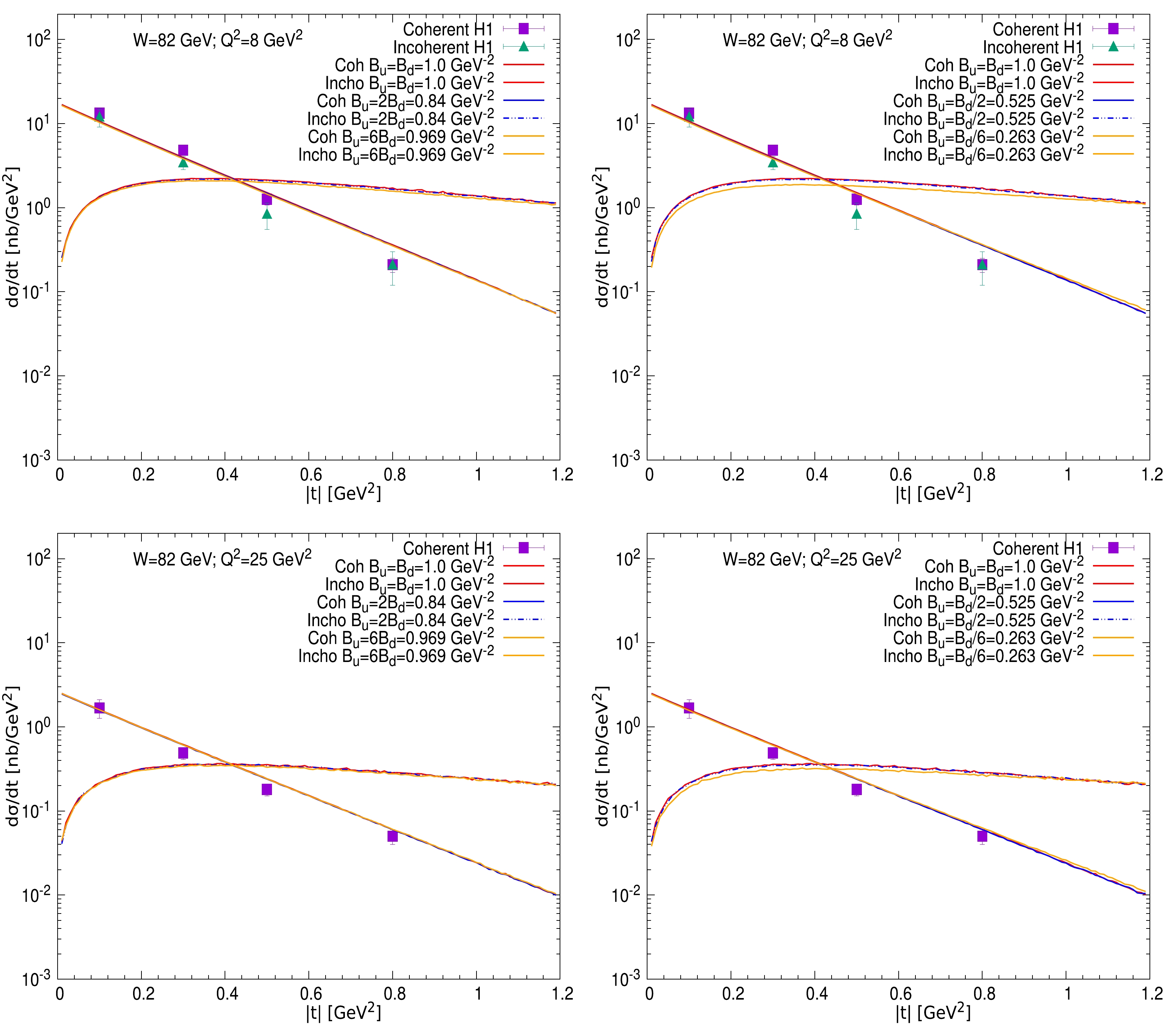
Figure 2. (color online) Coherent (solid curves) and incoherent (dashed curves) differential cross-sections of DVCS at
$ \sqrt{s}=82\; \mathrm{GeV} $ and$ Q^2=8\; \mathrm{GeV}^2 $ and$ Q^2=25\; \mathrm{GeV}^2 $ compared with the data from the H1 collaboration [53, 54]. The left hand side panel shows the results calculated with$ {B_u} \geq {B_d} $ , whereas the results in the right hand side panel are computed with${B_u} < {B_d}$ .The incoherent differential cross-section is obtained using the variance of the scattering amplitude; therefore, it is proportional to the variance of the proton profile, which renders it extremely sensitive to the spatial structure of the proton. The dashed curves in Fig. 2 show that the results computed with
$ {B_u} \geq {B_d} $ are consistent with each other (left hand panel), which agrees with the theoretical expectations, whereas the predictions calculated with$ {B_u} < {B_d} $ exhibit several discrepancies from each other (right hand panel). Keep in mind that the average width of the valence quarks is fixed. Only the dashed curves in the left hand panel of Fig. 2 are consistent with each other, which seems to indicate that the width of the profile density of the up quark is larger than or equal to that of the down quark. Figure 2 also shows that at the same collision energy, the discrepancies decrease as$ Q^2 $ increases. Moreover, the discrepancies shift to the relatively smaller t region compared to those obtained in vector meson productions in our previous study [37]. -
To observe the impact of energy on the outcomes obtained at the HERA energy, we study the DVCS process at EIC and LHeC energies. The coherent and incoherent differential cross-sections are calculated using our refined hot spot model in the cases of
$ {W=100\; \rm GeV} $ and$ {W=1000\;\rm GeV} $ with the same width parameters as shown in Fig. 2. Figure 3 presents the results calculated in the EIC energy. The upper panel of Fig. 3 shows the results calculated at${Q^2=5\; \rm GeV^2}$ , whereas the lower panel presents the predictions computed at${Q^2=10\; \rm GeV^2}$ . As shown, all the coherent differential cross-sections are consistent with each other regardless the varying width of the valence quarks, because the coherent cross-section can only reflect the overall average of the proton shape and not obtain deep information about the fine structure of the proton. Fortunately, the incoherent process can provide access to explore the internal structure of the proton. If proton shape flucutations (Eq. (16)) are not included in the calculation of the incoherent cross-section, the theoretical results will be several magnitudes smaller than the measurements [5]. By comparing the incoherent differential cross-sections in the right hand panel with those in the left hand panel in Fig. 3, we can see that there are significant differences. We use these differences to distinguish the shape of the valence quark. The incoherent differential cross-sections obtained in the case of${W_u}\geq {W_d}$ are consistent with each other, which is in agreement with the theoretical expectations. However, the incoherent differential cross-sections obtained in the case of${W_u} < {W_d}$ are inconsistent with each other. This outcome gives further support to the findings obtained in our previous study [37]. Note that the outcome obtained in this study is made more concrete because the wavefunction in the DVCS process can be precisely calculated by QED; therefore, the uncertainties from the modeling of the vector meson wavefunction are effectively removed.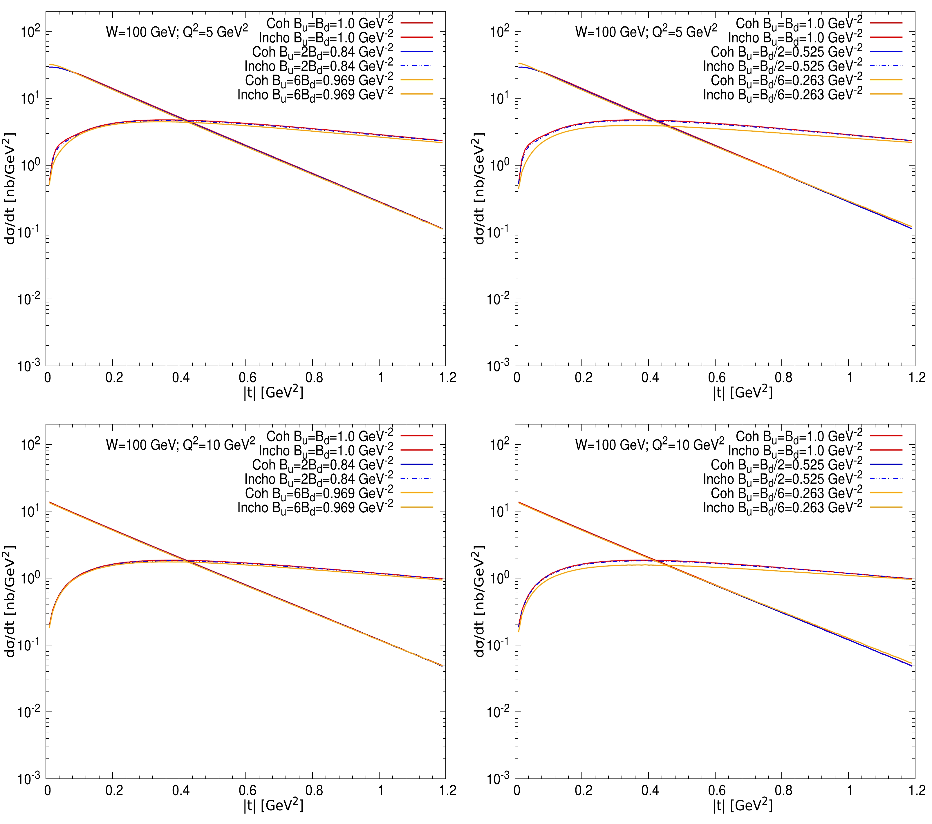
Figure 3. (color online) Coherent (solid curves) and incoherent (dashed curves) differential cross-sections of DVCS at
$ \sqrt{s}=100\; \mathrm{GeV} $ and$ Q^2=5\; \mathrm{GeV}^2 $ and$ Q^2=10\; \mathrm{GeV}^2 $ . All the parameters used in the calculations are the same as those used for Fig. 2. The numerical results in the left hand panel are calculated with${B_u} \geq {B_d}$ , whereas the predictions in right hand side panel are computed with${B_u} < {B_d}$ .The coherent and incoherent differential cross-sections at the LHeC energy are shown in Fig. 4. The parameters used to calculate the results in Fig. 4 are the same as those used for Fig. 3 except the collision energy. The outcomes extracted from Fig. 4 are almost the same as those from Fig. 3. However, an overall analysis from Fig. 2 to Fig. 4 reveals two significant results: (1) the discrepancies of the incoherent cross-sections presented in the right panel of these figures (computed in the
${W_u} < {W_d}$ case) decrease as$ Q^2 $ increases, and (2) the discrepancies between the incoherent cross-sections are broadened as the collision increases. This means that the EIC and LHeC can provide unprecedented opportunities to investigate the shape of the valence quark inside the proton.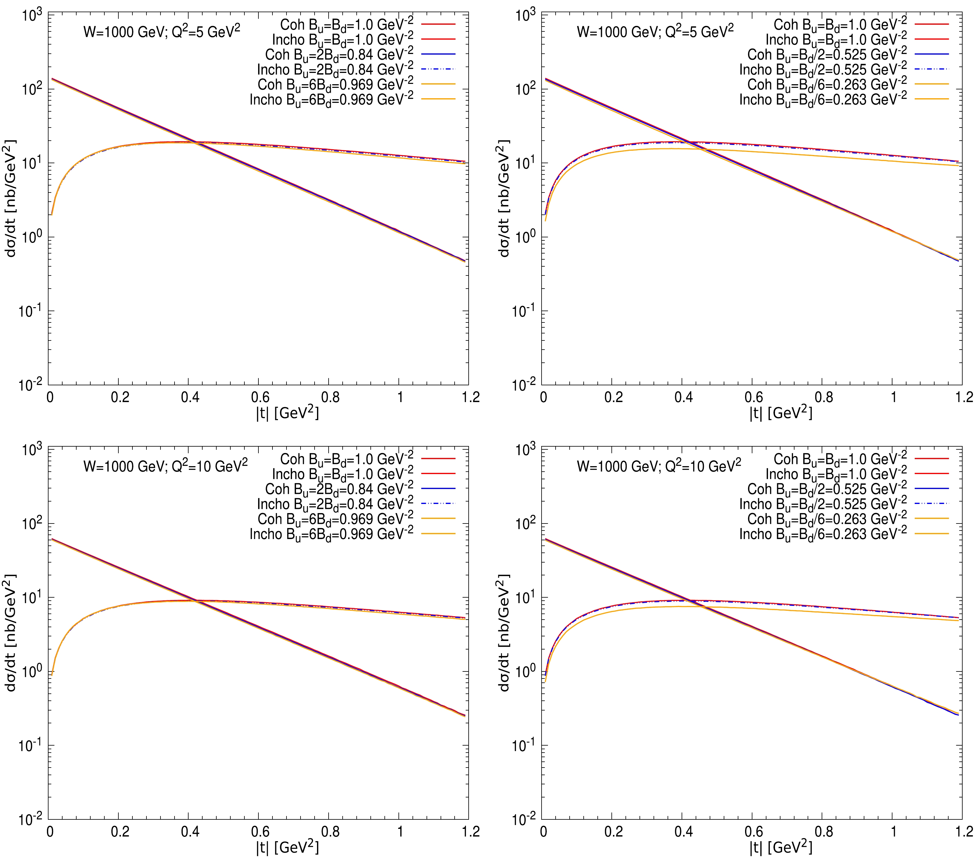
Figure 4. (color online) Coherent (solid curves) and incoherent (dashed curves) differential cross-sections of DVCS at
$ \sqrt{s}=1000\; \mathrm{GeV} $ and$ Q^2=5\; \mathrm{GeV}^2 $ and$ Q^2=10\; \mathrm{GeV}^2 $ . All the parameters used in the calculations are the same as those used for Fig. 2. The numerical results in the left hand panel are calculated with${B_u} \geq {B_d}$ , whereas the predictions in right hand side panel are computed with${B_u} < {B_d}$ . -
In the DVCS process, the distribution widths of the valence quarks of the proton are studied using the refined hot spot model. The theoretical uncertainties associated with the modeling of the vector meson wavefunction are removed because the overlap wavefunction used in this study can be precisely calculated by QED. As a consequence, the DVCS process can be used as a direct probe of QCD dynamics for the internal structure of the proton. The coherent and incoherent differential cross-sections of DVCS are calculated at HERA, EIC, and LHeC energies. The results show that the coherent cross-sections at each energy and
$ Q^2 $ are consistent with each other owing to the coherent cross-section only reflecting the average information of the proton. The predictions of the incoherent cross-section at each energy and$ Q^2 $ coincide with each other only in the case of${B_u}\geq {B_d}$ , which agrees with the theoretical expectations, whereas the corresponding ones are inconsistent in the case of${B_u} < {B_d}$ . Therefore, we can use this property as a probe to resolve the shape of the valence quarks inside the proton. Moreover, we find that the discrepancies between the incoherent cross-sections at each energy decrease as$ Q^2 $ increases, and these discrepancies are broadened from the HERA to LHeC energies. This outcome shows that the future EIC and LHeC will provide excellent access to study the internal spatial structure of the proton.In this study, we assume that the density profiles of up and down quarks obey a Gaussian distribution, although their distribution widths are treated individually. A recent study on lattice QCD showed that the distortions of the valence quarks of the proton were different, which inspires us to use different distributions to describe the density profile of up and down quarks in our future work.
Probing valence quark width of the proton in deeply virtual Compton scattering at high energies
- Received Date: 2023-12-05
- Available Online: 2024-05-15
Abstract: We use the refined hot spot model to study the valence quark shape of the proton with the deeply virtual Compton scattering at high energies in the color glass condensate framework. To investigate the individual valence quark shape, a novel treatment of the valence quark width is employed. We calculate the cross-sections for coherent and incoherent deeply virtual Compton scattering using, for the first time, different widths (


 DownLoad: