


 Abstract
 HTML
HTML Reference
 Related
 PDF
PDF


-
All particles predicted by the Standard Model (SM) have been found after the discovery of Higgs at the Large Hadron Collider (LHC) in 2012. However, some problems are still too difficult to solve using the SM, such as the non-zero neutrino mass and reasonable dark matter candidates. This indicates that new physics (NP) is needed to extend the SM. Since B meson rare decay processes
$ \bar B\rightarrow X_s\gamma $ and$ B_s^0\rightarrow \mu^+\mu^- $ are not affected by the uncertainties of non-perturbative QCD, research on B physics is particularly sensitive to exploring new physical effects beyond the SM. In Refs. [1−4], the average experimental data on the branching ratios of$ \bar B\rightarrow X_s\gamma $ and$ B_s^0\rightarrow \mu^+\mu^- $ are provided as$\begin{split} & {\rm{Br}}(\bar B\rightarrow X_s \gamma)=(3.49\pm0.19)\times 10^{-4},\\ & {\rm{Br}}(B_s^0\rightarrow \mu^+\mu^-)=(2.9_{-0.6}^{+0.7})\times10^{-9}. \end{split} $

(1) The branching ratios of
$ \bar B\rightarrow X_s\gamma $ and$ B_s^0\rightarrow \mu^+\mu^- $ predicted by the SM are [5−13]$\begin{split} &{\rm{Br}}(\bar B\rightarrow X_s \gamma)_{\rm{SM}}=(3.36\pm0.23)\times 10^{-4},\\ & {\rm{Br}}(B_s^0\rightarrow \mu^+\mu^-)_{\rm{SM}}=(3.23\pm0.27)\times10^{-9}, \end{split} $

(2) which coincides with the experimental data very well. Therefore, the NP contributions to
$ \bar B\rightarrow X_s\gamma $ and$B_s^0\rightarrow \mu^+\mu^-$ are limited strictly to the accurate measurements on the processes$ \bar B\rightarrow X_s\gamma $ and$ B_s^0\rightarrow \mu^+\mu^- $ .As one of the most famous extensions of the SM, the B meson rare decay process
$ \bar B\rightarrow X_s\gamma $ is analyzed in the MSSM [14−21]. In 1998, Ciuchini presented the QCD corrections to$ \bar B\rightarrow X_s\gamma $ at next-to-leading order (NLO) in the two-Higgs doublet model (THDM) [22]. Then, the two-loop QCD corrections was proposed in Ref. [23]. Besides the$ \bar B\rightarrow X_s\gamma $ process, there are also many existing studies on other B meson rare decay processes in the THDM [24−29]. Recently, the authors of Refs. [30−40] discussed the supersymmetric effects on the B meson rare decay processes. Meanwhile, Long et al. presented the computation of the flavor transition process$ b\rightarrow s\gamma $ [41]. The authors of Ref. [42investigated the two aspects of hadronic B decays, and then these processes in the case of CP violation have been discussed [43]. Moreover, many possibilities in searching for supersymmetry effects in different B meson rare decay processes have been proposed [44−46]. When investigating the processes of rare B decay, the supersymmetry effects are very interesting, and B decay can be conducive for us to understand the characteristics of the supersymmetry model in detail while limiting the parameter space [47, 48].TNMSSM is an extension of the next-to minimal supersymmetric standard model (NMSSM) containing two
$S U(2)_L$ triplets with hypercharge$ \pm1 $ , where the NMSSM introduces an additional scalar singlet compared with the MSSM [49]. As we know, MSSM can not solve the hierarchy problem and the μ problem. Thus, the new scalar singlet in the NMSSM is introduced to solve the μ problem [50, 51]. The main idea is that a bare μ term is forbidden, and the vacuum expectation value (VEV) of the singlet dynamically generates an effective μ term, which can coincide with the scale of soft supersymmetry breaking. However, the NMSSM, whose couplings are all perturbative up to the GUT scale, also fails to improve the little hierarchy problem [52−57]. Fortunately, the author of Ref. [49] solved these problems in the TNMSSM by introducing two scalar triplets with hypercharge$ Y=\pm1 $ , which naturally possesses a Higgs quartic coupling and would not decouple in the large$ \tan\beta $ limit. The tiny neutrino mass measured at the neutrino oscillation experiments can be obtained by applying a type II seesaw mechanism and a discrete flavor symmetry$ G_F $ in TNMSSM (i.e., the flavored-TNMSSM) [58]. In this work, we analyze the two loop electroweak corrections to$ \bar B\rightarrow X_s\gamma $ and$ B_s^0\rightarrow \mu^+\mu^- $ in the TNMSSM. Compared with the MSSM, new particle contents and interactions can make important contributions to the processes.The remainder of this paper is organized as follows: The superpotential, the soft breaking terms, and the mass matrices of singly-charged Higgs and CP-even Higgs in the TNMSSM are reviewed briefly in Sec. II. Sec. III and Sec. IV provides the corresponding Wilson coefficients and analytic expressions for
$ {\rm{Br}}(\bar B\rightarrow X_s\gamma) $ and$ {\rm{Br}}(B_s^0\rightarrow \mu^+\mu^-) $ . Sec. V analyzes the numerical results, and Sec. VI provides a summary of the study's findings. The corresponding matrix elements and the concrete expressions of the Wilson coefficients are collected in the appendices. -
There are different versions of TNMSSM, such as the triplet with hypercharge
$ Y=0 $ [59−61]. Here, we adopt the version of two triplets with hypercharge$ \pm1 $ . As mentioned before, the TNMSSM contains two$S U(2)_L$ triplets$ \hat T\sim(1,3,1) $ ,$ \hat {\bar T}\sim(-1,3,1) $ with$ Y=\pm1 $ and a SM gauge singlet$ \hat S\sim(0,1,1) $ . For the mass matrices and the interaction vertexes needed, we encode this version of TNMSSM in SARAH [62−66]. The chiral superfields for quarks and leptons are given by$\begin{split} &\hat{Q}=\left(\begin{array}{c}\hat U\\ \hat D\end{array}\right)\sim(1/6, 2, 3),\quad\; \hat{L}=\left(\begin{array}{c}\hat {\nu}\\ \hat E\end{array}\right)\sim(-1/2, 2, 1), \\ &\hat{U}^c\sim(-2/3, 1, 3),\quad\; \hat{D}^c\sim(1/3, 1, 3),\quad\; \hat E^c\sim(1, 1, 1), \end{split} $

(3) where we ignore the index of generations and the quantum numbers of
$ U(1)_Y $ ,$ S U(2)_L $ , and$ S U(3)_C $ are indicated in the bracket, respectively. Additionally, the expressions and quantum numbers of two Higgs triplets, two doublets, and one singlet are assigned as$ \begin{split} & \hat{T}=\left(\begin{array}{cc}\dfrac{1}{\sqrt2}T^+,&-T^{++}\\ T^0,&\dfrac{-1}{\sqrt2}T^+\end{array}\right)\sim (1, 3, 1),\\ & \hat{\bar T}=\left(\begin{array}{cc}\dfrac{1}{\sqrt2}{\bar T}^-,&-{\bar T}^0\\ {\bar T}^{--},&\dfrac{-1}{\sqrt2}{\bar T}^-\end{array}\right)\sim (-1, 3, 1), \\ & \hat{H_d}=\left(\begin{array}{c}H_d^0\\ H_d^-\end{array}\right)\sim (-1/2, 2, 1),\\ & \hat{H_u}=\left(\begin{array}{c}H_u^+\\ H_u^0\end{array}\right)\sim(1/2, 2, 1),\quad\;\hat S \sim(0, 1, 1). \end{split}$

(4) In the previous expressions,
$ T^0 $ and$ {\bar T}^0 $ are two complex neutral superfields, while$ T^+ $ ,$ \bar T^{--} $ are singly-charged Higgs, and$ T^{++} $ ,$ \bar T^{--} $ are doubly-charged Higgs.The superpotential of the TNMSSM
$ W_{\rm{TNMSSM}} $ contains two parts$ \begin{array}{*{20}{l}} W_{\rm{TNMSSM}}=W_{\rm{MSSM}}+W_{\rm{TS}}, \end{array} $

(5) with
$ \begin{array}{*{20}{l}} W_{\rm{MSSM}}=Y_u \hat U^c \hat H_u \cdot \hat Q -Y_d \hat D^c \hat H_d \cdot \hat Q -Y_e \hat E^c \hat H_d \cdot \hat L, \end{array} $

(6) where
$ W_{\rm{MSSM}} $ is the superpotential of the MSSM, and$ W_{\rm{TS}} $ explains the extended scalar sector, including two triplets and a SM gauge singlet,$ \begin{split} W_{\rm{TS}}=&\;\chi_d \hat H_d \cdot \hat T \hat H_d +\chi_u \hat H_u \cdot \hat {\bar T} \hat H_u +\frac{1}{3}\kappa \hat S \hat S \hat S +\lambda \hat S \hat H_u \cdot \hat H_d \\ & +\Lambda_T \hat S \mathrm{Tr}(\hat {\bar T} \hat T). \end{split}$

(7) Here, we also neglect the index of generations. From Eq. (6), we find that there are only two MSSM Higgs doublets coupled with fermion multiplet via Yukawa coupling. Then, the general soft breaking terms are given by
$ \begin{split} \mathcal{-L}_{\rm{soft}}=&\; m_{H_u}^2 |H_u|^2 +m_{H_d}^2 |H_d|^2 +m_S^2 |S|^2 +m_{T}^2 \mathrm{Tr}(|T|^2) \\ &+m_{\bar T}^2 \mathrm{Tr}(|\bar T|^2) +m_{Q}^2 |Q|^2 +m_{U}^2 |U|^2 +m_{D}^2 |D|^2 \\ &+(T_{\Lambda_T} S \mathrm{Tr}(T \bar T) +T_{\lambda} S H_u \cdot H_d +\frac{1}{3} T_{\kappa} S^3 \\ & -T_{\chi_u} H_u \cdot \bar T H_u -T_{\chi_d} H_d \cdot T H_d +\\ & T_{u,ij} \tilde{Q_j} \cdot H_u \tilde{U^c_i} -T_{d,ij} \tilde{Q_j} \cdot H_d \tilde{D^c_i} +H.c.), \end{split} $

(8) where
$ \begin{array}{*{20}{l}} H_u \cdot H_d =H_u^+ H_d^- -H_u^0 H_d^0, \end{array} $

(9) $ \begin{array}{*{20}{l}} H_d \cdot T H_d=\sqrt{2} H_d^- H_d^0 T^+ -(H_d^0)^2 T^0 -(H_d^-)^2 T^{++}, \end{array} $

(10) $ \begin{array}{*{20}{l}} H_u \cdot \bar T H_u=\sqrt{2} H_u^+ H_u^0 {\bar T}^- -(H_u^0)^2 {\bar T}^0 -(H_u^+)^2 {\bar T}^{--}. \end{array} $

(11) When the
$ Z_3 $ symmetry is imposed, the μ term only forms after the singlet S has obtained a VEV$ v_S $ as$ \mu=\dfrac{1}{\sqrt2} \lambda v_S $ . The coefficients in the Higgs sector are assumed to be real in the following calculations.The
$S U(2)_L\bigotimes U(1)_Y$ electroweak symmetry breaking occurs when the neutral parts of the Higgs fields obtain the VEVs$ \begin{split} & H_d^0=\frac{1}{\sqrt2} (v_d + \Re {H_d^0} +{\rm i} \Im {H_d^0}),\quad\; H_u^0=\frac{1}{\sqrt2} (v_u +\Re {H_u^0} +{\rm i} \Im {H_u^0}), \\ & T^0=\frac{1}{\sqrt2} (v_T + \Re {T^0} +{\rm i} \Im {T^0}),\quad\; {\bar T}^0=\frac{1}{\sqrt2} (v_{\bar T} +\Re {{\bar T}^0} +{\rm i} \Im {{\bar T}^0}), \\ & S=\frac{1}{\sqrt2} (v_S +\Re S +{\rm i} \Im S). \end{split} $

(12) Meanwhile, the VEVs of the triplets must be small to avoid a large ρ parameter correction [49], and the VEV of the singlet should be large enough to generate a large μ term like the case in the NMSSM [50]. In the TNMSSM, the mass of the Z gauge boson reads
$ M_Z^2=\frac{1}{4} (g_1^2 +g_2^2) (v_u^2+v_d^2 +4 v_T^2 +4 v_{\bar T}^2)=\frac{1}{4} (g_1^2 +g_2^2) v^2, $

(13) where
$ g_1 $ and$ g_2 $ represent the gauge coupling constants of$ U(1)_Y $ and$S U(2)_L$ , respectively. It can be seen from this that owing to the triplets, the electroweak symmetry breaking VEV for the doublets compared to MSSM is changed as$ \begin{array}{*{20}{l}} v=\sqrt {v_u^2+v_d^2 +4 v_T^2 +4 v_{\bar T}^2} \approx 246\; \rm GeV. \end{array} $

(14) Minimizing the Higgs scalar potential
$ \frac{\partial V}{\partial {v_u}}=\frac{\partial V}{\partial {v_d}}=\frac{\partial V}{\partial {v_T}}=\frac{\partial V}{\partial {v_{\bar T}}}=\frac{\partial V}{\partial {v_S}}=0, $

(15) we can deduce the squared mass matrices of the neutral and singly-charged Higgs. In the bases
$(H_d^{-}, H_u^{+,\ast}, {\bar T}^{-}, T^{+,\ast})$ and$ (H_d^{-,\ast}, H_u^{+}, {\bar T}^{-,\ast}, T^{+}) $ , the squared mass matrix for singly-charged Higgs can be expressed as$ \begin{array}{*{20}{l}} \mathcal{M}_{H^{\pm}}^2 = \left( \begin{array}{*{20}{c}} \mathcal{M}^2_{H_d^- H_d^{-,\ast}}&\mathcal{M}^2_{H_u^{+,\ast} H_d^{-,\ast}}&\mathcal{M}^2_{{\bar T}^- H_d^{-,\ast}}&\mathcal{M}^2_{T^{+,\ast} H_d^{-,\ast}}\\ \mathcal{M}^2_{H_d^- H_u^+}&\mathcal{M}^2_{H_u^{+,\ast} H_u^+}&\mathcal{M}^2_{{\bar T}^- H_u^+}&\mathcal{M}^2_{T^{+,\ast} H_u^+}\\ \mathcal{M}^2_{H_d^- {\bar T}^{-,\ast}}&\mathcal{M}^2_{H_u^{+,\ast} {\bar T}^{-,\ast}}&\mathcal{M}^2_{{\bar T}^- {\bar T}^{-,\ast}}&\mathcal{M}^2_{T^{+,\ast} {\bar T}^{-,\ast}}\\ \mathcal{M}^2_{H_d^- T^+}&\mathcal{M}^2_{H_u^{+,\ast} T^+}&\mathcal{M}^2_{{\bar T}^- T^+}&\mathcal{M}^2_{T^{+,\ast} T^+} \end{array} \right). \end{array} $

(16) The
$ 4 \times 4 $ squared mass matrix in Eq. (16) can be diagonalized by the unitary matrix$ Z^{H^{\pm}} $ $ \begin{array}{*{20}{l}} Z^{H^{\pm}} \mathcal{M}_{H^{\pm}}^2 Z^{H^{\pm},\dagger}=\mathcal{M}_{H^{\pm},\rm dia}^2. \end{array} $

(17) Then, we can get three mass eigenstates
$ (H_1^{\pm},H_2^{\pm},H_3^{\pm}) $ for the singly-charged Higgs and one state$ G^{\pm} $ for the massless Goldstone boson. Therefore, the TNMSSM has two more singly-charged Higgs owing to the triplets, with respect to MSSM. These newly defined singly-charged Higgs will bring contributions to loop corrections for$ \bar B\rightarrow X_s\gamma $ and$ B_s^0\rightarrow \mu^+\mu^- $ .At the tree level, the squared mass matrix for CP-even Higgs is given in the basis (
$ \Re H_d^0 $ ,$ \Re H_u^0 $ ,$ \Re S $ ,$ \Re T^0 $ ,$ \Re {\bar T}^0 $ ) as$ \begin{array}{*{20}{l}} \mathcal{M}_H^2=\left(\begin{array}{*{20}{c}} \mathcal{M}^2_{H_d^0 H_d^0}&\mathcal{M}^2_{H_u^0 H_d^0}&\mathcal{M}^2_{S H_d^0}&\mathcal{M}^2_{T^0 H_d^0}&\mathcal{M}^2_{{\bar T}^0 H_d^0}\\ \mathcal{M}^2_{H_d^0 H_u^0}&\mathcal{M}^2_{H_u^0 H_u^0}&\mathcal{M}^2_{S H_u^0}&\mathcal{M}^2_{T^0 H_u^0}&\mathcal{M}^2_{{\bar T}^0 H_u^0}\\ \mathcal{M}^2_{H_d^0 S}&\mathcal{M}^2_{H_u^0 S}&\mathcal{M}^2_{S S}&\mathcal{M}^2_{T^0 S}&\mathcal{M}^2_{{\bar T}^0 S}\\ \mathcal{M}^2_{H_d^0 T^0}&\mathcal{M}^2_{H_u^0 T^0}&\mathcal{M}^2_{S T^0}&\mathcal{M}^2_{T^0 T^0}&\mathcal{M}^2_{{\bar T}^0 T^0}\\ \mathcal{M}^2_{H_d^0 {\bar T}^0}&\mathcal{M}^2_{H_u^0 {\bar T}^0}&\mathcal{M}^2_{S {\bar T}^0}&\mathcal{M}^2_{T^0 {\bar T}^0}&\mathcal{M}^2_{{\bar T}^0 {\bar T}^0} \end{array}\right). \end{array} $

(18) The corresponding matrix elements of the squared mass matrices for singly-charged Higgs and CP-even Higgs are collected in Appendix A.
Including the leading-Log radiative corrections up to two loops for the stop and top sectors [67−69], the mass of the SM-like Higgs boson
$ m_h $ can be written as$ \begin{split} & m_h=\sqrt{(m_{h_1}^0)^2+\Delta m_h^2}, \\ & \Delta m_h^2=\frac{3m_t^4}{4 \pi^2 v^2}\Big[\tilde{t}+\frac{1}{2} \tilde{X}_t+\frac{1}{16\pi^2}\Big(\frac{3m_t^2}{2v^2}-32\pi\alpha_3\Big)\Big(\tilde{t}^2 +\tilde{X}_t \tilde{t}\Big)\Big],\\ & \tilde{t}=Log\frac{M_S^2}{m_t^2},\\&\tilde{X}_t=\frac{2\tilde{A}_t^2}{M_S^2}\Big(1-\frac{\tilde{A}_t^2}{12M_S^2}\Big), \end{split} $

(19) where
$ m_{h_1}^0 $ is the lightest tree-level Higgs boson mass,$ \alpha_3 $ is the running QCD coupling constant,$ M_S=\sqrt{m_{\tilde t_1}m_{\tilde t_2}} $ is the geometric mean of the stop masses$ m_{\tilde t_{1,2}} $ ,$ m_t $ is the top quark pole mass,$ \tilde{A}_t=A_t-\mu \cot\beta $ with$ A_t=T_{u,33} $ being the trilinear Higgs stop coupling, and μ is the Higgsino mass parameter.In the bases
$ (\tilde u_L, \tilde u_R) $ and$ (\tilde d_L, \tilde d_R) $ , we can obtain the squared mass matrices for Up-Squark and Down-Squark as$ \begin{array}{*{20}{l}} \mathcal{M}_{\tilde u}^2= \left(\begin{array}{cc}\mathcal{M}^2_{\tilde u_L \tilde{u}_L^\ast}&\mathcal{M}^2_{\tilde u_R \tilde{u}_L^\ast}\\ \mathcal{M}^2_{\tilde u_L \tilde{u}_R^\ast}&\mathcal{M}^2_{\tilde u_R \tilde{u}_R^\ast}\end{array}\right), \end{array} $

(20) $ \begin{array}{*{20}{l}} \mathcal{M}_{\tilde d}^2= \left(\begin{array}{cc}\mathcal{M}^2_{\tilde d_L \tilde{d}_L^\ast}&\mathcal{M}^2_{\tilde d_R \tilde{d}_L^\ast}\\ \mathcal{M}^2_{\tilde d_L \tilde{d}_R^\ast}&\mathcal{M}^2_{\tilde d_R \tilde{d}_R^\ast}\end{array}\right), \end{array} $

(21) where
$ \begin{aligned}[b] &\mathcal{M}^2_{\tilde u_L \tilde{u}_L^\ast}=-\frac{1}{24} (-3 g_2^2+g_1^2) (2 v_{\bar T}^2-2 v_T^2-v_u^2+v_d^2)\\ &\quad\quad\quad\;\;+\frac{1}{2} (2 m_q^2+v_u^2 Y_u^\dagger Y_u), \\ &\mathcal{M}^2_{\tilde u_L \tilde{u}_R^\ast}=\frac{1}{2} (\sqrt2 v_u T_u+Y_u (2 \chi_u v_u v_{\bar T}-\lambda v_d v_S)), \\ &\mathcal{M}^2_{\tilde u_R \tilde{u}_R^\ast}=\frac{1}{6}g_1^2 (2 v_{\bar T}^2-2 v_T^2-v_u^2+v_d^2)+\frac{1}{2}(2 m_u^2+v_u^2 Y_u Y_u^\dagger), \\ & \mathcal{M}^2_{\tilde d_L \tilde{d}_L^\ast}=-\frac{1}{24} (3 g_2^2+g_1^2) (2 v_{\bar T}^2-2 v_T^2-v_u^2+v_d^2)\\ &\quad\quad\quad\;\;+\frac{1}{2} (2 m_q^2+v_d^2 Y_d^\dagger Y_d), \\ &\mathcal{M}^2_{\tilde d_L \tilde{d}_R^\ast}=\frac{1}{2} (\sqrt2 v_d T_d+Y_d (2 \chi_d v_d v_T-\lambda v_u v_S)), \\ &\mathcal{M}^2_{\tilde d_R \tilde{d}_R^\ast}=\frac{1}{12}g_1^2 (-2 v_{\bar T}^2+2 v_T^2+v_u^2-v_d^2)+\frac{1}{2}(2 m_d^2+v_d^2 Y_d Y_d^\dagger). \end{aligned} $

(22) -
The effective Hamilton for the transition
$ b\rightarrow s $ at the hadronic scale can be described by$ \begin{split} H_{eff} =& -\frac{4G_F}{\sqrt{2}}V_{ts}^\ast V_{tb}\Big[C_1\mathcal{O}^c_1+C_2\mathcal{O}_2^c+\sum\limits_{i=3}^6\mathcal{O}_i+\sum\limits_{i=7}^{10}(C_i\mathcal{O}_i+C'_i\mathcal{O}'_i)\\ &+\sum\limits_{i=S,P}(C_i\mathcal{O}_i+C'_i\mathcal{O}'_i)\Big]. \end{split}$

(23) From the Refs. [70−75],
$ \mathcal{O}_i(i=1,...,10,S,P) $ and$ \mathcal{O}'_i(i=7,..., 10,S,P) $ are defined as$\begin{split} &{\cal O}_{_1}^c=(\bar{s}_{_L}\gamma_\mu T^au_{_L})(\bar{u}_{_L}\gamma^\mu T^ab_{_L})\;,\;\; {\cal O}_{_2}^c=(\bar{s}_{_L}\gamma_\mu u_{_L})(\bar{u}_{_L}\gamma^\mu b_{_L})\;,\\ &{\cal O}_{_3}=(\bar{s}_{_L}\gamma_\mu b_{_L})\sum\limits_q(\bar{q}\gamma^\mu q)\;,\;\; {\cal O}_{_4}=(\bar{s}_{_L}\gamma_\mu T^ab_{_L})\sum\limits_q(\bar{q}\gamma^\mu T^aq)\;,\\ &{\cal O}_{_5}=(\bar{s}_{_L}\gamma_\mu\gamma_\nu\gamma_\rho b_{_L})\sum\limits_q(\bar{q}\gamma^\mu\gamma^\nu\gamma^\rho q)\;,\;\; \\ &{\cal O}_{_6}=(\bar{s}_{_L}\gamma_\mu\gamma_\nu\gamma_\rho T^ab_{_L})\sum\limits_q(\bar{q}\gamma^\mu\gamma^\nu\gamma^\rho T^aq)\;,\\ &{\cal O}_{_7}={e\over 16\pi^2}m_{_b}(\bar{s}_{_L}\sigma_{_{\mu\nu}}b_{_R})F^{\mu\nu}\;,\;\; {\cal O}_{_7}'={e\over 16\pi^2}m_{_b}(\bar{s}_{_R}\sigma_{_{\mu\nu}}b_{_L})F^{\mu\nu}\;,\\ &{\cal O}_{_8}={g_{_s}\over 16\pi^2}m_{_b}(\bar{s}_{_L}\sigma_{_{\mu\nu}}T^ab_{_R})G^{a,\mu\nu}\;,\;\; \\ &{\cal O}_{_8}'={g_{_s}\over 16\pi^2}m_{_b}(\bar{s}_{_R}\sigma_{_{\mu\nu}}T^ab_{_L})G^{a,\mu\nu}\;,\\ &{\cal O}_{_9}={e^2\over g_{_s}^2}(\bar{s}_{_L}\gamma_\mu b_{_L})\bar{l}\gamma^\mu l\;,\;\; {\cal O}_{_9}'={e^2\over g_{_s}^2}(\bar{s}_{_R}\gamma_\mu b_{_R})\bar{l}\gamma^\mu l\;,\\ &{\cal O}_{_{10}}={e^2\over g_{_s}^2}(\bar{s}_{_L}\gamma_\mu b_{_L})\bar{l}\gamma^\mu\gamma_5 l\;,\;\; {\cal O}_{_{10}}'={e^2\over g_{_s}^2}(\bar{s}_{_R}\gamma_\mu b_{_R})\bar{l}\gamma^\mu\gamma_5 l\;,\\ &{\cal O}_{_S}={e^2\over16\pi^2}m_{_b}(\bar{s}_{_L}b_{_R})\bar{l}l\;,\;\; {\cal O}_{_S}'={e^2\over16\pi^2}m_{_b}(\bar{s}_{_R}b_{_L})\bar{l}l\;,\;\;\\ &{\cal O}_{_P}={e^2\over16\pi^2}m_{_b}(\bar{s}_{_L}b_{_R})\bar{l}\gamma_5l\;,\;\; {\cal O}_{_P}'={e^2\over16\pi^2}m_{_b}(\bar{s}_{_R}b_{_L})\bar{l}\gamma_5l\;, \end{split} $

(24) where
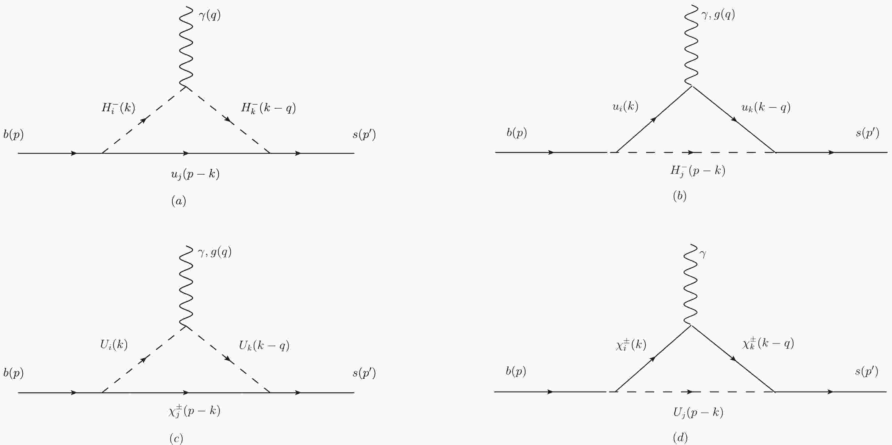
$ g_s $ represents the strong coupling,$ F^{\mu\nu} $ is the electromagnetic field strength tensor,$ G^{\mu\nu} $ is the gluon field strength tensor, and$ T^a\,(a=1,...,8) $ are the$S U(3)$ generators.As shown in Fig. 1, the main one-loop Feynman diagrams contributing to the process
$ \bar{B}\rightarrow X_s\gamma $ in the TNMSSM are mediated by newly defined up-squarks, singly-charged Higgs, and charginos. Compared to the MSSM, these new definitions of singly-charged Higgs and charginos will affect the prediction of the process$ \bar{B}\rightarrow X_s\gamma $ . In the TNMSSM, the one loop Wilson coefficients corresponding to Fig. 1 are$ C_{7,NP}^{(a)}(\mu_{\rm EW}) $ ,$ C_{7,NP}^{(b)}(\mu_{\rm EW}) $ ,$ C_{7,NP}^{(c)}(\mu_{\rm EW}) $ , and$ C_{7,NP}^{(d)}(\mu_{\rm EW}) $ , and their concrete expressions can be obtained from Appendix B.
Figure 1. The one loop Feynman diagrams contributing to
$ \bar{B}\rightarrow X_s\gamma $ in the TNMSSM.At the two loop level, we consider the corrections from the closed fermion loop in Fig. 2. In Fig. 2, newly defined neutralinos, charginos, and doubly-charged chargino in the TNMSSM bring new contributions to
$ \bar{B}\rightarrow X_s\gamma $ compared to the MSSM. Then, the two loop Wilson coefficients$ C_{7,NP}^{WW}(\mu_{\rm EW}) $ ,$ C_{8,NP}^{WW}(\mu_{\rm EW}) $ ,$ C_{7,NP}^{WH}(\mu_{\rm EW}) $ , and$ C_{8,NP}^{WH}(\mu_{\rm EW}) $ from Fig. 2 are also collected in Appendix B.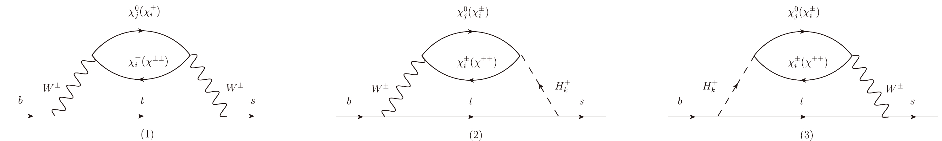
Figure 2. The related two loop diagrams in which a closed heavy fermion loop is attached to virtual
$ W^\pm $ bosons or$ H^\pm $ , where a real photon or gluon is attached in all possible ways.In addition,
$ C_{8g,NP}(\mu_{\rm EW}),\;C_{8g,NP}^{\prime}(\mu_{\rm EW}),\;C_{8,NP}^{WW}(\mu_{\rm EW}),\; C_{8,NP}^{WH}(\mu_{\rm EW}) $ are Wilson coefficients of the process$ b\rightarrow sg $ in the TNMSSM, which can make contributions to the process$ b\rightarrow s\gamma $ through QCD running. Similarly, the Wilson coefficients of the process$ b\rightarrow sg $ in the EW scale can be written as$\begin{split} &C_{8g,NP}(\mu_{\rm EW})=[C_{7,NP}^{(b)}(\mu_{\rm EW})+C_{7,NP}^{(c)}(\mu_{\rm EW})]/Q_u\\ &\quad\quad\quad\quad\quad\;\;\; +C_{8,NP}^{WW}(\mu_{\rm EW})+ C_{8,NP}^{WH}(\mu_{\rm EW}), \\ &C_{8g,NP}^{\prime}(\mu_{\rm EW})=C_{8g,NP}(\mu_{\rm EW})(L\leftrightarrow R), \end{split} $

(25) where
$ Q_u=2/3 $ .Based on the Wilson coefficients above, the branching ratio of
$ \bar{B}\rightarrow X_s\gamma $ in the TNMSSM can be given by$ \begin{array}{*{20}{l}} {\rm{Br}}(\bar{B}\rightarrow X_s\gamma)=R\Big(|C_{7\gamma}(\mu_b)|^2 +N(E_\gamma)\Big)\;, \end{array} $

(26) where the overall factor
$ R=2.47\times10^{-3} $ , and the nonperturbative contribution$ N(E_\gamma)=(3.6\pm0.6)\times10^{-3} $ [76].$ C_{7\gamma}(\mu_b) $ is defined as$ \begin{array}{*{20}{l}} C_{7\gamma}(\mu_b)=C_{7\gamma,SM}(\mu_b)+C_{7,NP}(\mu_b), \end{array} $

(27) where we choose the hadron scale
$ \mu_b=2.5 $ GeV, and at NNLO level, the SM contribution is$ C_{7\gamma,SM}(\mu_b) = -0.3689 $ [76−78]. The Wilson coefficients for NP at the bottom quark scale can be written as [79, 80]$ \begin{array}{*{20}{l}} C_{7,NP}(\mu_b)\approx0.5696 C_{7,NP}(\mu_{\rm EW})+0.1107 C_{8,NP}(\mu_{\rm EW}), \end{array} $

(28) where
$ \begin{split} &C_{7,NP}(\mu_{\rm EW})=C_{7,NP}^{(a)}(\mu_{\rm EW})+C_{7,NP}^{(b)}(\mu_{\rm EW})+ C_{7,NP}^{(c)}(\mu_{\rm EW})\\ &\quad\quad\quad\quad\quad\; +C_{7,NP}^{(d)}(\mu_{\rm EW})+C_{7,NP}^{\prime(a)}(\mu_{\rm EW})+C_{7,NP}^{\prime(b)}(\mu_{\rm EW})\\ &\quad\quad\quad\quad\quad\; +C_{7,NP}^{\prime (c)}(\mu_{\rm EW})+C_{7,NP}^{\prime(d)}(\mu_{\rm EW})+C_{7,NP}^{WW}(\mu_{\rm EW})\\ &\quad\quad\quad\quad\quad\; +C_{7,NP}^{WH}(\mu_{\rm EW}),\\ &C_{8,NP}(\mu_{\rm EW})=C_{8g,NP}(\mu_{\rm EW})+C_{8g,NP}^{\prime}(\mu_{\rm EW}) +C_{8,NP}^{WW}(\mu_{\rm EW})\\ &\quad\quad\quad\quad\quad\;+C_{8,NP}^{WH}(\mu_{\rm EW}). \end{split}$

(29) -
Figure 3 shows the main one loop vertex and box diagrams contributing to the process
$ B_s^0\rightarrow \mu^+\mu^- $ in the TNMSSM. In Fig. 3, newly defined up-squarks and pseudo-scalar Higgs bosons will make new contributions to the branching ratio$ {\rm{Br}}(B_s^0\rightarrow \mu^+\mu^-) $ compared to the MSSM. Considering Fig. 2 and Fig. 3, the Wilson coefficients corresponding to the process$ B_s^0\rightarrow \mu^+\mu^- $ at the EW scale can be written as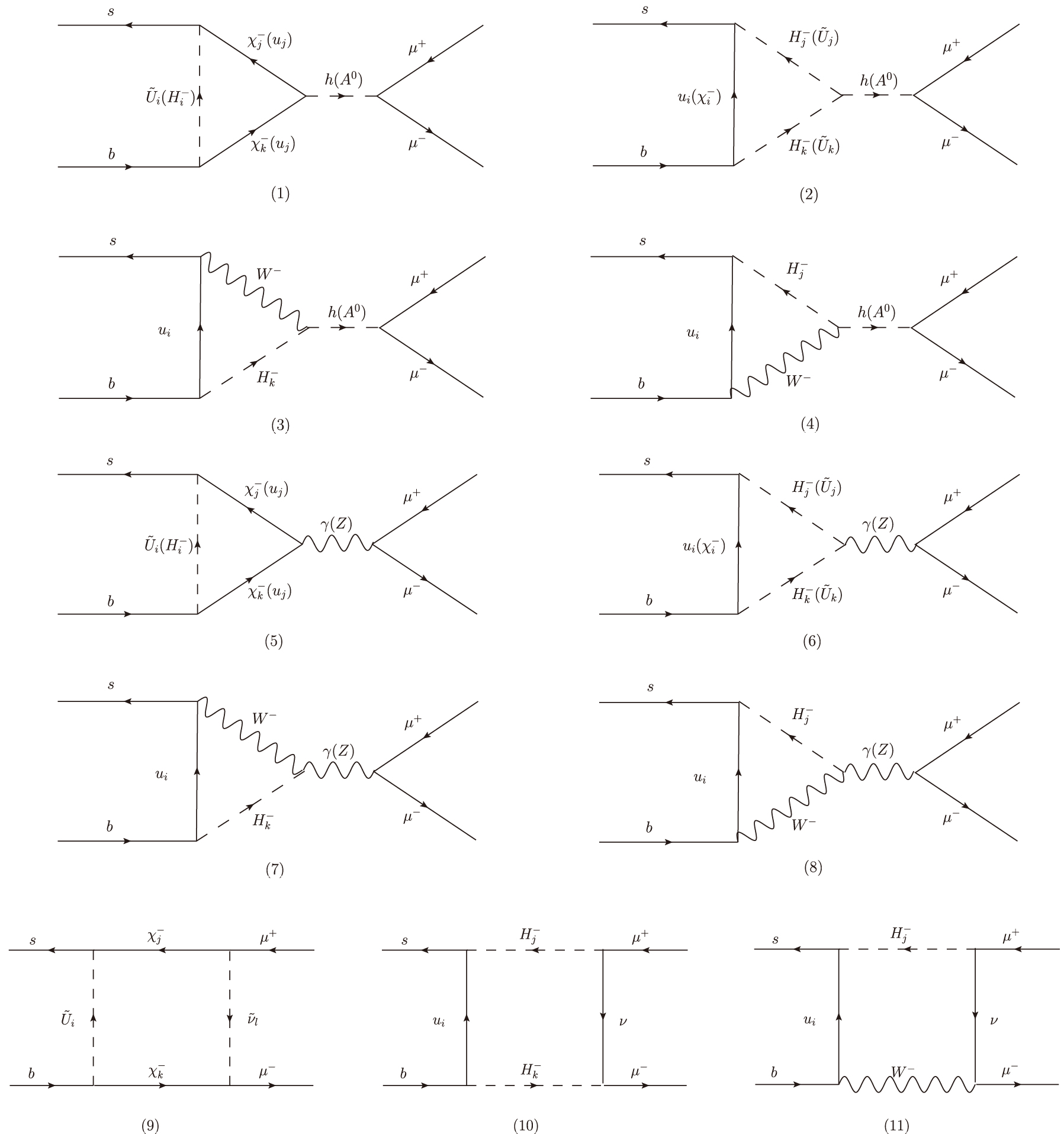
Figure 3. The one loop vertex and box diagrams contributing to
$ B_s^0\rightarrow \mu^+\mu^- $ in the TNMSSM.$ \begin{split}\\[-12pt] &C_{_{S,NP}}(\mu_{_{\rm{EW}}})=\frac{\sqrt{2}s_{_W}c_{_W}}{4m_be^3V_{ts}^*V_{tb}}\Big[C_{_{S,NP}}^{(1)}(\mu_{_{\rm{EW}}})+C_{_{S,NP}}^{(2)}(\mu_{_{\rm{EW}}})+C_{_{S,NP}}^{(3)}(\mu_{_{\rm{EW}}})+C_{_{S,NP}}^{(4)}(\mu_{_{\rm{EW}}})+C_{_{S,NP}}^{(6)}(\mu_{_{\rm{EW}}})+C_{_{S,NP}}^{(9)}(\mu_{_{\rm{EW}}})+C_{_{S,NP}}^{(11)}(\mu_{_{\rm{EW}}})\Big],\\ &C_{_{S,NP}}^\prime(\mu_{_{\rm{EW}}})=C_{_{S,NP}}(\mu_{_{\rm{EW}}})(L\leftrightarrow R),\\ &C_{_{P,NP}}(\mu_{_{\rm{EW}}})=\frac{\sqrt{2}s_{_W}c_{_W}}{4m_be^3V_{ts}^*V_{tb}}\Big[C_{_{P,NP}}^{(1)}(\mu_{_{\rm{EW}}})+C_{_{P,NP}}^{(2)}(\mu_{_{\rm{EW}}})+C_{_{P,NP}}^{(3)}(\mu_{_{\rm{EW}}})+C_{_{P,NP}}^{(4)}(\mu_{_{\rm{EW}}})+C_{_{P,NP}}^{(6)}(\mu_{_{\rm{EW}}})+C_{_{P,NP}}^{(9)}(\mu_{_{\rm{EW}}})+C_{_{P,NP}}^{(11)}(\mu_{_{\rm{EW}}})\Big],\\ &C_{_{P,NP}}^\prime(\mu_{_{\rm{EW}}})=-C_{_{P,NP}}(\mu_{_{\rm{EW}}})(L\leftrightarrow R), \end{split} $ 
$ \begin{split} &C_{_{9,NP}}(\mu_{_{\rm{EW}}})=\frac{\sqrt{2}s_{_W}c_{_W}g_{_s}^2}{64\pi^2e^3V_{ts}^*V_{tb}}\Big[C_{_{9,NP}}^{(5)}(\mu_{_{\rm{EW}}})+C_{_{9,NP}}^{(6)}(\mu_{_{\rm{EW}}})+C_{_{9,NP}}^{(7)}(\mu_{_{\rm{EW}}})+C_{_{9,NP}}^{(8)}(\mu_{_{\rm{EW}}})+C_{_{9,NP}}^{(9)}(\mu_{_{\rm{EW}}})+C_{_{9,NP}}^{(10)}(\mu_{_{\rm{EW}}})+C_{_{9,NP}}^{WW}(\mu_{_{\rm{EW}}})\Big]\;,\\ &C_{_{9,NP}}^\prime(\mu_{_{\rm{EW}}})=C_{_{9,NP}}(\mu_{_{\rm{EW}}})(L\leftrightarrow R),\\ &C_{_{10,NP}}(\mu_{_{\rm{EW}}})=\frac{\sqrt{2}s_{_W}c_{_W}g_{_s}^2}{64\pi^2e^3V_{ts}^*V_{tb}}\Big[C_{_{10,NP}}^{(5)}(\mu_{_{\rm{EW}}})+C_{_{10,NP}}^{(6)}(\mu_{_{\rm{EW}}})+C_{_{10,NP}}^{(7)}(\mu_{_{\rm{EW}}})+C_{_{10,NP}}^{(8)}(\mu_{_{\rm{EW}}})+C_{_{10,NP}}^{(9)}(\mu_{_{\rm{EW}}})+C_{_{10,NP}}^{(10)}(\mu_{_{\rm{EW}}})+C_{_{10,NP}}^{WW}(\mu_{_{\rm{EW}}})\Big]\;,\\ &C_{_{10,NP}}^\prime(\mu_{_{\rm{EW}}})=-C_{_{10,NP}}(\mu_{_{\rm{EW}}})(L\leftrightarrow R). \end{split} $

(30) All of the Wilson coefficients calculated above are gauge invariant and the concrete expressions on the right side of Eq. (30) are collected in Appendix B. In addition, the renormalization group equations can also evolve the Wilson coefficients from EW scale
$\mu_{\rm EW}$ to hadronic scale$ \mu\sim m_b $ . To obtain hadronic matrix elements conveniently, we define effective coefficients as [72]$ \begin{split} &C_7^{\rm eff}=\frac{4\pi}{\alpha_s}C_7-\frac{1}{3}C_3-\frac{4}{9}C_4-\frac{20}{3}C_5-\frac{80}{9}C_6,\\ &C_8^{\rm eff}=\frac{4\pi}{\alpha_s}C_8+C_3-\frac{1}{6}C_4+20C_5-\frac{10}{3}C_6,\\ &C_9^{\rm eff}=\frac{4\pi}{\alpha_s}C_9+Y(q^2),\;\;C_{10}^{\rm eff}=\frac{4\pi}{\alpha_s}C_{10},\\ &{C'}_{7,8,9,10}^{\rm eff}=\frac{4\pi}{\alpha_s}{C'}_{7,8,9,10}. \end{split}$

(31) The Wilson coefficients at hadronic energy scale from the SM to Next-to-Next-to-Logarithmic (NNLL) accuracy are shown in Table 1. The renormalization group equations are written as
$C_{_7}^{\rm eff,SM}$ 

$C_{_8}^{\rm eff,SM}$ 

$C_{_9}^{\rm eff,SM}-Y(q^2)$ 

$C_{_{10} }^{\rm eff,SM}$ 

$ -0.304 $ 

$ -0.167 $ 

$ 4.211 $ 

$ -4.103 $ 

Table 1. Wilson coefficients from the SM to NNLL accuracy at hadronic scale
$ \mu=m_{_b}\simeq4.65 $ GeV.$ \begin{split} &\overrightarrow{C}_{_{NP}}(\mu)=\widehat{U}(\mu,\mu_0)\overrightarrow{C}_{_{NP}}(\mu_0) \;,\\ & \overrightarrow{C^\prime}_{_{NP}}(\mu)=\widehat{U^\prime}(\mu,\mu_0) \overrightarrow{C^\prime}_{_{NP}}(\mu_0) \end{split} $

(32) with
$ \begin{split} &\overrightarrow{C}_{_{NP}}^{T}=\Big(C_{_{1,NP}},\;\cdots,\;C_{_{6,NP}}, C_{_{7,NP}}^{\rm eff},\;C_{_{8,NP}}^{\rm eff},\;C_{_{9,NP}}^{\rm eff}-Y(q^2),\; C_{_{10,NP}}^{\rm eff}\Big) \;,\\ & \overrightarrow{C}_{_{NP}}^{\prime,\;T}=\Big(C_{_{7,NP}}^{\prime,\;\rm eff},\; C_{_{8,NP}}^{\prime,\;\rm eff},\;C_{_{9,NP}}^{\prime,\;\rm eff},\; C_{_{10,NP}}^{\prime,\;\rm eff}\Big)\;, \end{split} $

(33) and
$\begin{split} &\widehat{U}(\mu,\mu_0)\simeq1-\Big[{1\over2\beta_0}\ln{\alpha_{_s}(\mu)\over \alpha_{_s}(\mu_0)}\Big]\widehat{\gamma}^{(0)T} \;,\\ &\widehat{U^\prime}(\mu,\mu_0)\simeq1-\Big[{1\over2\beta_0}\ln{\alpha_{_s}(\mu)\over \alpha_{_s}(\mu_0)}\Big]\widehat{\gamma^\prime}^{(0)T}\;, \end{split} $

(34) where Ref. [81] provided the anomalous dimension matrices as
$ \begin{array}{*{20}{l}}\\[-3pt] \widehat{\gamma}^{(0)}=\left(\begin{array}{cccccccccc} -4&\displaystyle{8\over3}&0&-\displaystyle{2\over9}&0&0&-\displaystyle{208\over243}&\displaystyle{173\over162}&-\displaystyle{2272\over729}&0\\ 12&0&0&\displaystyle{4\over3}&0&0&\displaystyle{416\over81}&\displaystyle{70\over27}&\displaystyle{1952\over243}&0\\ 0&0&0&-\displaystyle{52\over3}&0&2&-\displaystyle{176\over81}&\displaystyle{14\over27}&-\displaystyle{6752\over243}&0\\ 0&0&-\displaystyle{40\over9}&-\displaystyle{100\over9}&\displaystyle{4\over9}&\displaystyle{5\over6}&-\displaystyle{152\over243}&-\displaystyle{587\over162}&-\displaystyle{2192\over729}&0\\ 0&0&0&-\displaystyle{256\over3}&0&20&-\displaystyle{6272\over81}&\displaystyle{6596\over27}&-\displaystyle{84032\over243}&0\\ 0&0&-\displaystyle{256\over9}&\displaystyle{56\over9}&\displaystyle{40\over9}&-\displaystyle{2\over3}&\displaystyle{4624\over243}&\displaystyle{4772\over81}&-\displaystyle{37856\over729}&0\\ 0&0&0&0&0&0&\displaystyle{32\over3}&0&0&0\\ 0&0&0&0&0&0&-\displaystyle{32\over9}&\displaystyle{28\over3}&0&0\\ 0&0&0&0&0&0&0&0&0&0\\ 0&0&0&0&0&0&0&0&0&0\\ \end{array}\right) \;, \quad \widehat{\gamma^\prime}^{(0)}=\left(\begin{array}{cccc} \displaystyle{32\over3}&0&0&0\\ -\displaystyle{32\over9}&\displaystyle{28\over3}&0&0\\ 0&0&0&0\\0&0&0&0\\ \end{array}\right)\;.\\ \end{array} $ 
(35) Based on the Wilson coefficients above, the branching ratio of
$ B_s^0\rightarrow \mu^+\mu^- $ can be given by$ {\rm{Br}}(B_s^0\rightarrow \mu^+\mu^-)=\frac{\tau_{B_s^0}}{16\pi}\frac{|\mathcal{M}_s|^2}{M_{B_s^0}}\sqrt{1-\frac{4m_{\mu}^2}{M_{B_s^0}^2}}, $

(36) where
$M_{B_s^0}=5.367 \;\rm GeV$ denotes the mass of neutral meson$ B_s^0 $ , and$\tau_{B_s^0}=1.466(31)\;{\rm{ps}}$ denotes its lifetime. Moreover, the squared amplitude can be written as$ \begin{array}{*{20}{l}} |\mathcal{M}_s|^2=16G_F^2|V_{tb}V_{ts}^*|^2M_{B_s^0}^2\Big[|F_S^s|^2+|F_P^s+2m_{\mu}F_A^s|^2\Big], \end{array} $

(37) with
$ F_S^s=\frac{\alpha_{\rm EW}(\mu_b)}{8\pi}\frac{m_b M_{B_s^0}^2}{m_b+m_s}f_{B_s^0}(C_S-C_S'), $

(38) $ F_P^s=\frac{\alpha_{\rm EW}(\mu_b)}{8\pi}\frac{m_b M_{B_s^0}^2}{m_b+m_s}f_{B_s^0}(C_P-C_P'), $

(39) $ F_A^s=\frac{\alpha_{\rm EW}(\mu_b)}{8\pi}f_{B_s^0}\Big[C_{10}^{\rm eff}(\mu_b)-C_{10}^{\prime\rm eff}(\mu_b)\Big], $

(40) where
$ f_{B_s^0}=(227\pm8){\rm{MeV}} $ denote the decay constants. -
This section provides the numerical discussion of the branching ratios of B meson rare decays
$ \bar B\rightarrow X_s\gamma $ and$ B_s^0\rightarrow \mu^+\mu^- $ by considering the latest multiple experimental constraints of particles. This includes that the SM-like Higgs mass$ m_h $ is kept around$ 125.25\;{\rm{GeV}} $ , the neutralino mass is limited to more than$ 116\;{\rm{GeV}} $ , the chargino mass is limited to more than$ 1100\;{\rm{GeV}} $ , the slepton mass is limited to more than$ 700\;{\rm{GeV}} $ , and the squark mass is maintained at the TeV order of magnitude [1, 82−89]. Additionally, the first two generations of squarks are strongly constrained by direct searches at the LHC [90, 91]. However, compared to the previous two generations, the mass of the third generation squark, which can affect the mass of SM-like Higgs, does not suffer strong constraints. Therefore, we take$ m_{\tilde{q}}=m_{\tilde{u}}=$ ${\rm diag}(2, 2, m_{\tilde t})$ TeV, and the discussion about the observed Higgs signal in Ref. [92] limits$ m_{\tilde t}\gtrsim1.5\;{\rm{TeV}} $ . For simplicity, we also choose$ T_{u_{1,2}}=Y_{u_{1,2}} A_{u_{1,2}} $ ,$ A_{u_{1,2}}=1\;{\rm{TeV}} $ . As a key parameter,$ T_{u_3}=A_t $ clearly affects the SM-like Higgs mass and the numerical calculation. In order to obtain reasonable numerical results, we need to find some sensitive parameters for discussion. Similarly to the MSSM [93], the NP contributions to the branching ratios$ {\rm{Br}}(\bar B\rightarrow X_s\gamma) $ and$ {\rm{Br}}(B_s^0\rightarrow \mu^+\mu^-) $ also depend on$ \tan\beta $ ,$ A_t $ , and a singly-charged Higgs mass. Moreover, according to their significant impact on a singly-charged Higgs mass, neutralino mass and chargino mass, we found three other new parameters κ, λ, and$ T_{\lambda} $ that can affect$ {\rm{Br}}(\bar B\rightarrow X_s\gamma) $ and$ {\rm{Br}}(B_s^0\rightarrow \mu^+\mu^-) $ in the TNMSSM. We will plot the relational and scatter diagrams and explore the effects of these parameters on the branching ratios and the allowed ranges between λ, κ, and$ T_{\lambda} $ .By considering the experimental constraints described above, we adopt the parameters in the following numerical calculation as
$ \begin{split} &\chi_d=\chi_u=0.1,\;\Lambda_T=0.6,\;\tan\beta'=5,\\ &M_1=1\;{\rm{TeV}},\;m_{\tilde t}=1.6\;{\rm{TeV}},\\ &M_2=\mu=1.2\;{\rm{TeV}},\;T_{\chi_d}=T_{\chi_u}=-500\;{\rm{GeV}},\;\\ &T_{\kappa}=-300\;{\rm{GeV}},\;T_{\Lambda_T}=100\;{\rm{GeV}}. \end{split} $

(41) To illustrate the effects of
$ A_t $ and$ \tan\beta $ on the branching ratios, we take$ \lambda=0.4,\;\kappa=0.6,\;T_{\lambda}=100\;{\rm{GeV}} $ and plot the graph of$ {\rm{Br}}(\bar B\rightarrow X_s\gamma) $ and$ {\rm{Br}}(B_s^0\rightarrow \mu^+\mu^-) $ varying with$ A_t $ in Fig. 4 for$ \tan\beta=10$ (solid line),$\tan\beta=25 $ (dashed line), and$\tan\beta=40 $ (dotted line). The gray area denotes the experimental 1σ bounds in Eq. (1). Fig. 4(a) shows that$ {\rm{Br}}(\bar B\rightarrow X_s\gamma) $ decreases as$ A_t $ increases, and the slope of evolution is steeper as$ \tan\beta $ increases. In Fig. 4(b), we can see that the variation relationship between$ A_t $ and$ {\rm{Br}}(B_s^0\rightarrow \mu^+\mu^-) $ is almost parabolic. Moreover, when$ \tan\beta $ is larger,$ A_t $ is limited strongly in the smaller range by the experimental data on$ {\rm{Br}}(B_s^0\rightarrow \mu^+\mu^-) $ . This indicates that the NP can provide considerable contributions to$ {\rm{Br}}(B_s^0\rightarrow \mu^+\mu^-) $ for large$ \tan\beta $ and$ A_t $ .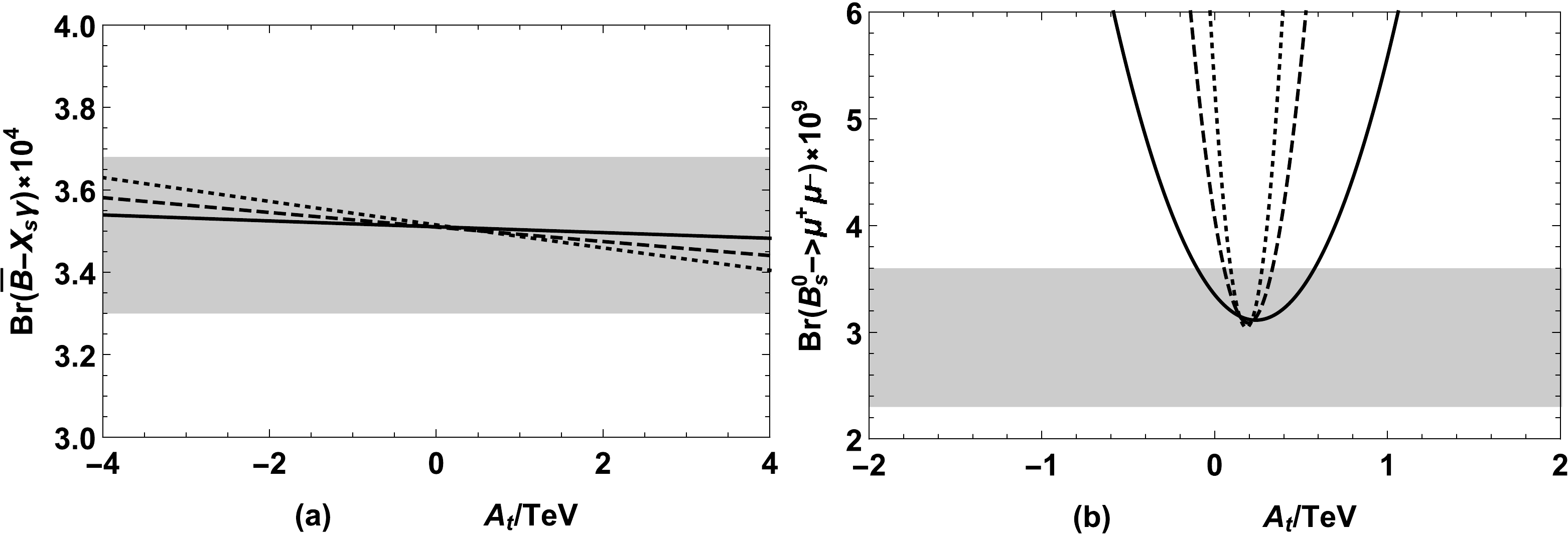
Figure 4. (a)
$ {\rm{Br}}(\bar B\rightarrow X_s\gamma) $ and (b)$ {\rm{Br}}(B_s^0\rightarrow \mu^+\mu^-) $ versus$ A_t $ for$ \tan\beta=10\;({\rm{solid \;line}}),\;\tan\beta=25\;({\rm{dashed \;line}}),\;\tan\beta=40\;({\rm{dotted \;line}}) $ , where the gray area denotes the experimental 1σ interval.To see the effects of
$ \lambda,\;\kappa, $ and$ T_{\lambda} $ on the branching ratios, we first take$ \lambda=0.4,\;\tan\beta=5,\;A_t=0.5\;{\rm{TeV}} $ and plot the graph of$ {\rm{Br}}(\bar B\rightarrow X_s\gamma) $ and$ {\rm{Br}}(B_s^0\rightarrow \mu^+\mu^-) $ varying with$ T_{\lambda} $ in Fig. 5, for$\kappa=0.4 $ (solid line),$ \kappa=0.5$ (dashed line), and$\kappa=0.6 $ (dotted line), respectively. Then, we take$ T_{\lambda}=100\;{\rm{GeV}},\;\tan\beta=5,\;A_t=0.5\;{\rm{TeV}} $ and plot the graph of$ {\rm{Br}}(\bar B\rightarrow X_s\gamma) $ and$ {\rm{Br}}(B_s^0\rightarrow \mu^+\mu^-) $ varying with κ in Fig. 6, for$ \lambda=0.9 $ (solid line),$\lambda=0.7$ (dashed line), and$\lambda=0.5 $ (dotted line), respectively. The gray area denotes the experimental 1σ bounds. Fig. 5 shows that$ {\rm{Br}}(\bar B\rightarrow X_s\gamma) $ and$ {\rm{Br}}(B_s^0\rightarrow \mu^+\mu^-) $ increase as$ T_{\lambda} $ decreases when$ T_{\lambda} $ is negative and the three lines mix together for a large$ T_{\lambda} $ . Thus, it can be seen that when a smaller κ is taken, the smaller range of$ T_{\lambda} $ is limited, and a large$ T_{\lambda} $ eliminate the influence of κ. In Fig. 6(a),$ {\rm{Br}}(\bar B\rightarrow X_s\gamma) $ decreases gradually as κ increases, and κ is less affected by λ. However, from Fig. 6(b),$ {\rm{Br}}(B_s^0\rightarrow \mu^+\mu^-) $ decreases dramatically near$ \kappa=0.4 $ for$ \lambda=0.5 $ ,$ \kappa=0.6 $ for$ \lambda=0.7 $ , and$ \kappa=0.9 $ for$ \lambda=0.9 $ , respectively. This indicates that λ has strong limitations for κ, which will be discussed in the following by the depicted scatter plots.
Figure 5. (a)
$ {\rm{Br}}(\bar B\rightarrow X_s\gamma) $ and (b)$ {\rm{Br}}(B_s^0\rightarrow \mu^+\mu^-) $ versus$ T_{\lambda} $ for$ \kappa=0.4\;({\rm{solid \;line}}),\;\kappa=0.5\;({\rm{dashed \;line}}),\;\kappa=0.6\;({\rm{dotted \;line}}) $ when$ \lambda=0.4 $ . The gray area denotes the experimental 1σ interval.
Figure 6. (a)
$ {\rm{Br}}(\bar B\rightarrow X_s\gamma) $ and (b)$ {\rm{Br}}(B_s^0\rightarrow \mu^+\mu^-) $ versus κ for$ \lambda=0.9\;({\rm{solid \;line}}),\;\lambda=0.7\;({\rm{dashed \;line}}),\;\lambda=0.5\;({\rm{dotted \;line}}) $ when$ T_{\lambda}=100\;{\rm{GeV}} $ . The gray area denotes the experimental 1σ interval.Meanwhile, when comparing and reflecting the specific differences between the one loop and two loop corrections to
$ \bar B\rightarrow X_s\gamma $ and$ B_s^0\rightarrow \mu^+\mu^- $ , we take$ T_{\lambda}= $ 100 GeV,$ \lambda=0.7 $ and plot the graph of$ {\rm{Br}}(\bar B\rightarrow X_s\gamma) $ and$ {\rm{Br}}(B_s^0\rightarrow \mu^+\mu^-) $ varying with κ in Fig. 7. The solid and dashed lines denote the two loop and one loop predictions, respectively. Figure 7(a) shows that the relative corrections from the two loop diagrams to one loop corrections of$ {\rm{Br}}(\bar B\rightarrow X_s\gamma) $ can reach approximately$ 4\% $ , which can produce a more precise prediction for the process$ \bar B\rightarrow X_s\gamma $ . In Fig. 7(b), we can see that the two lines almost overlap, which indicates that the two loop corrections are negligible compared with the one loop corrections. Therefore, in analyzing the numerical calculations above, we always use the more precise two loop predictions.
Figure 7. The comparison graph of the two loop (solid lines) results and one loop (dashed lines) results when
$ \lambda=0.7,\;T_{\lambda}=100\;{\rm{GeV}} $ , where the gray area denotes the experimental 1σ interval.Now, to revealing how
$ \lambda,\;\kappa, $ and$ T_{\lambda} $ is constrained by the experimental measurements of B meson rare decays, we scan the sensitive parameters, considering the experimental constraints above and$ {\rm{Br}}(\bar B\rightarrow X_s\gamma) $ ,$ {\rm{Br}}(B_s^0\rightarrow \mu^+\mu^-) $ within one standard deviation. The random ranges of the input parameters are as follows:$ \begin{split} &\tan\beta=(1,40),\;\lambda=(0.01,0.99),\;\kappa=(0.01,0.99),\\ &\mu=(1.1,1.5)\;{\rm{TeV}},\;T_{\lambda}=(-1,1)\;{\rm{TeV}},\\&A_t=(-4,4)\;{\rm{TeV}}. \end{split} $

(42) Then, we plot the allowed ranges of κ versus λ,
$ T_{\lambda} $ versus λ, and κ versus$ T_{\lambda} $ in Fig. 8. Figure 8(a) shows that the vast majority of points are concentrated in the areas$ \kappa>\lambda $ , and the number of points gradually decreases as$ \kappa<\lambda $ . In Fig. 8(b), we find that the density of points decreases as λ increases, and this phenomenon is more obvious when$ \lambda>0.6 $ . As shown in Fig. 8(c), the negative range of$ T_{\lambda} $ is gradually limited when$ \kappa<0.6 $ . In conclusion, to maintain$ {\rm{Br}}(\bar B\rightarrow X_s\gamma) $ and$ {\rm{Br}}(B_s^0\rightarrow \mu^+\mu^-) $ within the experimental 1σ interval,$ \lambda,\;\kappa $ should preferably be in the range$ \lambda<0.6 $ ,$ \kappa>0.6 $ , and have a positive$ T_{\lambda} $ .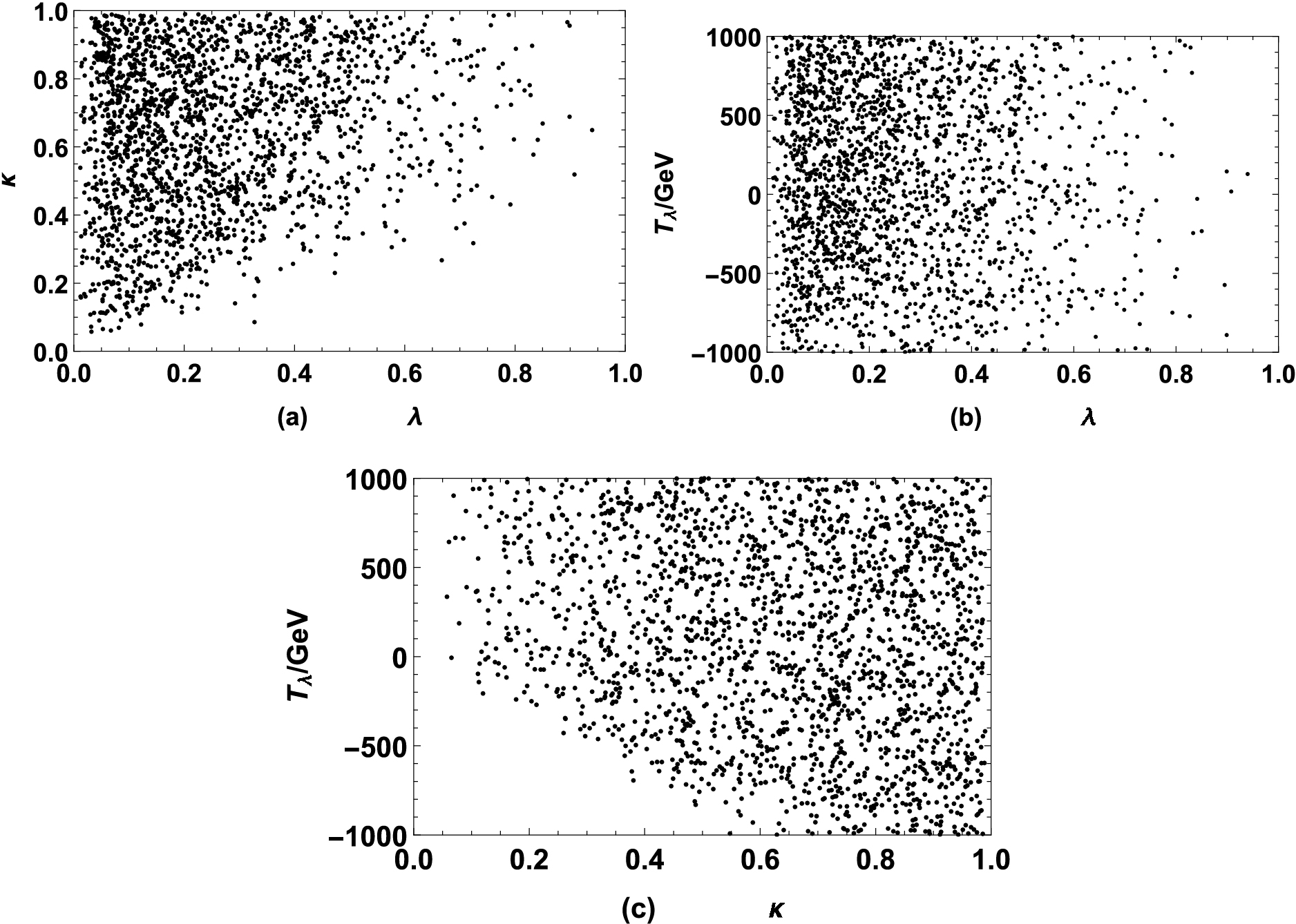
Figure 8. Scanning the parameter space in Eq.(42) and keeping
$ {\rm{Br}}(\bar B\rightarrow X_s\gamma) $ ,$ {\rm{Br}}(B_s^0\rightarrow \mu^+\mu^-) $ in the experimental 1σ interval, the allowed ranges of$ \kappa-\lambda $ (a),$ T_{\lambda}-\lambda $ (b),$ T_{\lambda}-\kappa $ (c) are plotted. -
B meson rare decays are sensitive to searching on NP beyond the SM. In this study, we investigate the two loop electroweak corrections for the processes
$ \bar B\rightarrow X_s\gamma $ and$ B_s^0\rightarrow \mu^+\mu^- $ in the TNMSSM, which extends the MSSM with two triplets and one singlet. Considering the constraints from the observed Higgs signal and the updated experimental data of the branching ratios, the numerical results indicate that the corrections from the two loop diagrams for the process$ \bar B\rightarrow X_s\gamma $ in the TNMSSM can reach approximately$ 4\% $ , which can produce a more precise theoretical prediction. Moreover, the NP effects in the TNMSSM can fit the experimental data for the rare decays$ \bar B\rightarrow X_s\gamma $ and$ B_s^0\rightarrow \mu^+\mu^- $ , and the corresponding parameter space is limited strictly by considering$ {\rm{Br}}(\bar B\rightarrow X_s\gamma) $ and$ {\rm{Br}}(B_s^0\rightarrow \mu^+\mu^-) $ in the experimental 1σ intervals. The new parameters$ \lambda,\;\kappa,\;T_{\lambda} $ in the TNMSSM significantly influence the theoretical predictions of$ {\rm{Br}}(\bar B\rightarrow X_s\gamma) $ ,$ {\rm{Br}}(B_s^0\rightarrow \mu^+\mu^-) $ . Further, to maintain$ {\rm{Br}}(\bar B\rightarrow X_s\gamma) $ and$ {\rm{Br}}(B_s^0\rightarrow \mu^+\mu^-) $ within the experimental 1σ interval,$ \lambda,\;\kappa $ should preferably be in the range$ \lambda<0.6 $ ,$ \kappa>0.6 $ and have a positive$ T_{\lambda} $ . -
Our deepest gratitude goes to Professor Tai-Fu Feng for his sincere guidance on this research.
-
The matrix elements of the squared mass matrix for singly-charged Higgs are given by
$ \begin{split} &\mathcal{M}^2_{H_d^- H_d^{-,\ast}}=\frac{\sqrt2}{2} T_{\lambda} \tan\beta v_S -\sqrt2 T_{\chi_d} v_T +\frac{1}{4} g_2^2 (\tan^2\beta v_d^2 +2 v_T^2 -2 v_{\bar T}^2) -\frac{1}{2} \lambda^2 \tan^2\beta v_d^2 \\ & \quad\quad\quad\quad\; +\Lambda_T \chi_d v_S v_{\bar T} -2 {\chi_d}^2 v_T^2 +\frac{1}{2} \lambda \tan\beta (\kappa v_S^2 -\Lambda_T v_T v_{\bar T} +2 v_S (\chi_d v_T +\chi_u v_{\bar T})), \\ & \mathcal{M}^2_{H_u^{+,\ast} H_u^+}=\frac{1}{4 \tan\beta} (2 \sqrt2 T_{\lambda} v_S+g_2^2 \tan\beta (v_d^2 -2 v_T^2 +2 v_{\bar T}^2) -2 \tan\beta (2 \sqrt2 T_{\chi_u} v_{\bar T} +\lambda^2 v_d^2 \\ & \quad\quad\quad\quad\; -2 \Lambda_T \chi_u v_S v_T +4 \chi_u^2 v_{\bar T}^2) +2 \lambda (\kappa v_S^2 -\Lambda_T v_T v_{\bar T} +2 (\chi_d v_T +\chi_u v_{\bar T}) v_S)), \\ & \mathcal{M}^2_{{\bar T}^- {\bar T}^{-,\ast}}=\frac{1}{4} \Big(2 \sqrt2 T_{\Lambda_T} \tan\beta' v_S -g_2^2 v_d^2 +2 g_2^2 v_T^2 +2 \kappa \Lambda_T \tan\beta' v_S^2 -2 \Lambda_T^2 v_T^2 +\frac{2 \Lambda_T \chi_d v_d^2 v_S}{v_{\bar T}} \\ & \quad\quad\quad\quad\; -2 \tan\beta \lambda v_d^2 \Big(\Lambda_T \tan\beta' -\frac{2 \chi_u v_S}{v_{\bar T}}\Big) +\tan^2\beta v_d^2 \Big(-\frac{2 \sqrt2 T_{\chi_u}}{v_{\bar T}} +g_2^2 -4 \chi_u^2\Big)\Big), \\ & \mathcal{M}^2_{T^{+,\ast} T^+}=\frac{1}{4} \Big(-\frac{2 \sqrt2 T_{\chi_d} v_d^2}{v_T} +g_2^2 (v_d^2 -\tan^2\beta v_d^2 +2 v_{\bar T}^2) +2 \Big(\frac{\sqrt2 T_{\Lambda_T} v_S}{\tan\beta'} \\ & \quad\quad\quad\quad\; +\frac{\kappa \Lambda_T v_S^2}{\tan\beta'} -\frac{\lambda \Lambda_T \tan\beta v_d^2}{\tan\beta'} -\Lambda_T^2 v_{\bar T}^2 -2 \chi_d^2 v_d^2 +\frac{\tan\beta v_d^2 v_S}{v_T} (2 \lambda \chi_d +\tan\beta \Lambda_T \chi_u)\Big)\Big), \\ & \mathcal{M}^2_{H_u^{+,\ast} H_d^{-,\ast}}=\mathcal{M}^2_{H_d^- H_u^+}=\frac{1}{4} (g_2^2 \tan\beta v_d^2 +2 \sqrt2 T_{\lambda} v_S -2 \lambda (-\kappa v_S^2 +\lambda \tan\beta v_d^2 +\Lambda_T v_T v_{\bar T})), \\ & \mathcal{M}^2_{{\bar T}^- H_d^{-,\ast}}=\mathcal{M}^2_{H_d^- {\bar T}^{-,\ast}}=\frac{1}{2 \sqrt2} v_d (g_2^2 v_{\bar T}-2 (\Lambda_T \chi_d+\lambda \chi_u \tan\beta) v_S), \\& \mathcal{M}^2_{T^{+,\ast} H_d^{-,\ast}}=\mathcal{M}^2_{H_d^- T^+}=\frac{1}{4} v_d (-4 T_{\chi_d}+\sqrt2 (g_2^2 v_T+2 \chi_d (\lambda \tan\beta v_S -2 \chi_d v_T))), \\ & \mathcal{M}^2_{{\bar T}^- H_u^+}=\mathcal{M}^2_{H_u^{+,\ast} {\bar T}^{-,\ast}}=\frac{1}{4} v_d (-4 \tan\beta T_{\chi_u} +2 \sqrt2 \lambda \chi_u v_S +\sqrt2 \tan\beta v_{\bar T} (g_2^2 -4 \chi_u^2)), \\ & \mathcal{M}^2_{T^{+,\ast} H_u^+}=\mathcal{M}^2_{H_u^{+,\ast} T^+}=\frac{v_d}{2 \sqrt2} (g_2^2 \tan\beta v_T -2 v_S (\lambda \chi_d +\tan\beta \Lambda_T \chi_u)), \\ & \mathcal{M}^2_{T^{+,\ast} {\bar T}^{-,\ast}}=\mathcal{M}^2_{{\bar T}^- T^+}=\frac{1}{2} (\sqrt2 T_{\Lambda_T} v_S +g_2^2 v_T v_{\bar T} -\Lambda_T (-\kappa v_S^2 +\lambda \tan\beta v_d^2 +\Lambda_T v_T v_{\bar T})), \end{split} \tag{A1}$ 
where
$ \tan\beta=\dfrac{v_u}{v_d} $ and$ \tan\beta'=\dfrac{v_T}{v_{\bar T}} $ .The matrix elements of the squared mass matrix for CP-even Higgs are written as
$\begin{split} &\mathcal{M}^2_{H_d^0 H_d^0}=\frac{1}{4} ((g^2 +8 \chi_d^2) v_d^2+2 \tan\beta v_S N -2 \lambda \Lambda_T \tan\beta \tan\beta' v_{\bar T}^2), \\ & \mathcal{M}^2_{H_u^0 H_u^0}=\frac{1}{4} ((g^2 +8 \chi_u^2) v_d^2+\frac{2 v_S}{\tan\beta} N -2 \lambda \Lambda_T \frac{\tan\beta'}{\tan\beta} v_{\bar T}^2), \\ & \mathcal{M}^2_{H_u^0 H_d^0}=\frac{1}{4} ((-g^2 +4 \lambda^2) \tan\beta v_d^2-2 v_S N +2 \lambda \Lambda_T \tan\beta' v_{\bar T}^2), \\ & \mathcal{M}^2_{S S}=\frac{1}{2} \bigg(\frac{\tan\beta v_d^2}{v_S} (x+\sqrt2 T_{\lambda}+2 n)+\frac{1}{v_S} (\Lambda_T \chi_d v_d^2 v_{\bar T}+\sqrt2 T_{\Lambda_T} \tan\beta' v_{\bar T}^2) +\sqrt2 T_{\kappa} v_S+4 \kappa^2 v_S^2\bigg), \\ & \mathcal{M}^2_{S H_d^0}=\frac{-1}{2} v_d (\sqrt2 \tan\beta T_{\lambda}-2 \lambda^2 v_S+2 \tan\beta n+2 \tan\beta \lambda \kappa v_S+2 \Lambda_T \chi_d v_{\bar T}), \\ & \mathcal{M}^2_{S H_u^0}=-\frac{T_{\lambda} v_d}{\sqrt2}-v_d (\lambda v_S (\kappa-\lambda \tan\beta)+n+x), \\ & \mathcal{M}^2_{T^0 T^0}=g^2 \tan^2\beta' v_{\bar T}^2+\frac{1}{2 \tan\beta' v_{\bar T}} (\sqrt2 T_{\Lambda_T} v_S v_{\bar T}-\sqrt2 T_{\chi_d} v_d^2+\kappa \Lambda_T v_S^2 v_{\bar T} +\tan\beta v_d^2 (2 \lambda \chi_d v_S+\tan\beta \Lambda_T \chi_u v_S-\lambda \Lambda_T v_{\bar T})), \\& \mathcal{M}^2_{H_d^0 T^0}=\frac{v_d}{2} (2 \sqrt2 T_{\chi_d}-g^2 \tan\beta' v_{\bar T}+\lambda \tan\beta (\Lambda_T v_{\bar T}-2 \chi_d v_S)+8 \tan\beta' \chi_d^2 v_{\bar T}), \\& \mathcal{M}^2_{H_u^0 T^0}=\frac{v_d}{2} (g^2 \tan\beta \tan\beta' v_{\bar T}+\lambda \Lambda_T v_{\bar T}-2 \lambda \chi_d v_S-2 \tan\beta \Lambda_T \chi_u v_S), \\ & \mathcal{M}^2_{S T^0}=-\frac{T_{\Lambda_T} v_{\bar T}}{\sqrt2}+ \Lambda_T v_S v_{\bar T} (-\kappa+\tan\beta' \Lambda_T) -\frac{1}{2} \tan\beta v_d^2 (2 \lambda \chi_d +\tan\beta \Lambda_T \chi_u), \\ & \mathcal{M}^2_{{\bar T}^0 {\bar T}^0}=g^2 v_{\bar T}^2+\frac{1}{2} \tan\beta' v_S (\sqrt2 T_{\Lambda_T}+\kappa \Lambda_T v_S)+\frac{1}{2 v_{\bar T}} (-\sqrt2 \tan^2\beta T_{\chi_u} v_d^2 +\Lambda_T \chi_d v_d^2 v_S+\lambda \tan\beta v_d^2 (-\tan\beta' \Lambda_T v_{\bar T}+2 \chi_u v_S)), \\ & \mathcal{M}^2_{H_d^0 {\bar T}^0}=\frac{1}{2} v_d (g^2 v_{\bar T}+\lambda \Lambda_T \tan\beta \tan\beta' v_{\bar T}-2 \Lambda_T \chi_d v_S-2 \lambda \chi_u \tan\beta v_S), \\& \mathcal{M}^2_{H_u^0 {\bar T}^0}=\frac{1}{2} v_d (2 \sqrt2 \tan\beta T_{\chi_u}+\lambda (\Lambda_T \tan\beta v_{\bar T}-2 \chi_u v_S)-\tan\beta v_{\bar T} (g^2-8 \chi_u^2)), \\ & \mathcal{M}^2_{S {\bar T}^0}=\Lambda_T^2 v_S v_{\bar T}-\frac{1}{2} \tan\beta' v_{\bar T} (\sqrt2 T_{\Lambda_T}+2 \kappa \Lambda_T v_S)-\frac{1}{2} v_d^2 (\Lambda_T \chi_d+2 \tan\beta \lambda \chi_u), \\ & \mathcal{M}^2_{T^0 {\bar T}^0}=\frac{1}{2} (-\sqrt2 T_{\Lambda_T} v_S-2 g^2 \tan\beta' v_{\bar T}^2-\kappa \Lambda_T v_S^2+\lambda \Lambda_T \tan\beta v_d^2+2 \tan\beta' \Lambda_T^2 v_{\bar T}^2), \end{split} \tag{A2}$

where
$ g^2=g_{_1}^2+g_{_2}^2 $ ,$ N=\sqrt2 T_{\lambda}+\kappa \lambda v_S+2 \lambda \chi_d \tan\beta' v_{\bar T}+2 \lambda \chi_u v_{\bar T} $ ,$ x=\Lambda_T \chi_u \tan\beta \tan\beta' v_{\bar T} $ ,$ n=\lambda v_{\bar T} (\tan\beta' \chi_d+\chi_u) $ . -
The one loop Wilson coefficients for the process
$ \bar B\rightarrow X_s\gamma $ are written as$ C_{7,NP}^{(a)}(\mu_{\rm EW})=\sum\limits_{H^-_i,u_j}\frac{s_W^2}{2e^2V^*_{ts}V_{tb}} \Big\{ \frac{1}{2}C_{H^-_i\bar s u_j}^R C_{H^-_i b \bar u_j}^{L}[-I_3(x_{u_j},x_{H^-_i})+I_4(x_{u_j},x_{H^-_i})]+\frac{m_{u_j}}{m_b}C_{H^-_i\bar s u_j}^L C_{H^-_i b \bar u_j}^{L}[-I_1(x_{u_j},x_{H^-_i})+I_3(x_{u_j},x_{H^-_i})]\Big\}, \tag{B1}$

$ \begin{aligned}[b] C_{7,NP}^{(b)}(\mu_{\rm EW})=&\sum\limits_{H^-_j,u_i}\frac{s_W^2}{3e^2V^*_{ts}V_{tb}} \Big\{ \frac{1}{2}C_{H^-_j\bar s u_i}^R C_{H^-_j b \bar u_i}^{L}[-I_1(x_{u_i},x_{H^-_j})+2I_3(x_{u_i},x_{H^-_j})-I_4(x_{u_i},x_{H^-_j})]+\frac{m_{u_i}}{m_b}C_{H^-_j\bar s u_i}^L C_{H^-_j b \bar u_i}^{L}[I_1(x_{u_i},x_{H^-_j})\\ &-I_2(x_{u_i},x_{H^-_j})-I_3(x_{u_i},x_{H^-_j})]\Big\}, \end{aligned} \tag{B2}$

$ \begin{aligned}[b] C_{7,NP}^{(c)}(\mu_{\rm EW})=&\sum\limits_{U^+_i,\chi^-_j}\frac{s_W^2}{3e^2V^*_{ts}V_{tb}} \Big\{ \frac{1}{2}C_{U^+_i\bar s \chi^-_j}^R C_{U^+_i b \bar \chi^-_j}^{L}[-I_3(x_{\chi^-_j},x_{U^+_i})+I_4(x_{\chi^-_j},x_{U^+_i})]\\ &+\frac{m_{\chi^-_j}}{m_b}C_{U^+_i\bar s \chi^-_j}^L C_{U^+_i b \bar \chi^-_j}^{L}[-I_1(x_{\chi^-_j},x_{U^+_i})+I_3(x_{\chi^-_j},x_{U^+_i})]\Big\}, \end{aligned} \tag{B3}$

$ \begin{aligned}[b] C_{7,NP}^{(d)}(\mu_{\rm EW})=&\sum\limits_{U^+_j,\chi^-_i}\frac{s_W^2}{2e^2V^*_{ts}V_{tb}} \Big\{ \frac{1}{2}C_{U^+_i\bar s \chi^-_i}^R C_{U^+_j b \bar \chi^-_i}^{L}[-I_1(x_{\chi^-_i},x_{U^+_j})+2I_2(x_{\chi^-_i},x_{U^+_j})\\ &-I_4(x_{\chi^-_i},x_{U^+_j})]+\frac{m_{\chi^-_i}}{m_b}C_{U^+_j\bar s \chi^-_i}^L C_{U^+_j b \bar \chi^-_i}^{L}[I_1(x_{\chi^-_i},x_{U^+_j})-I_2(x_{\chi^-_i},x_{U^+_j})\\ &-I_3(x_{\chi^-_i},x_{U^+_j})]\Big\}, \end{aligned} \tag{B4}$

$ \begin{array}{*{20}{l}} C_{7,NP}^{(\xi)}(\mu_{\rm EW})=C_{7,NP}^{\prime (\xi)}(\mu_{\rm EW})(L\leftrightarrow R), (\xi=a,b,c,d), \end{array} \tag{B5}$

where
$ C_{XYZ}^{L,R} $ denotes the constant parts of the interaction vertices about particles$ XYZ $ , L, and R, representing the left and right-handed parts, respectively.Denoting
$ x_i=\dfrac{m_i^2}{m_W^2} $ , the concrete expressions for$ I_k(k=1,...,4) $ can be given as$\begin{split} &I_1(x_1,x_2)=\frac{1+{\rm{ln}} x_2}{(x_2-x_1)}+\frac{x_1 {\rm{ln}} x_1-x_2 {\rm{ln}} x_2}{(x_2-x_1)^2},\\ &I_2(x_1,x_2)=-\frac{1+{\rm{ln}} x_1}{(x_2-x_1)}-\frac{x_1 {\rm{ln}} x_1-x_2 {\rm{ln}} x_2}{(x_2-x_1)^2},\\ &I_3(x_1,x_2)=\frac{1}{2}\Big[\frac{3+2{\rm{ln}} x_2}{(x_2-x_1)}-\frac{2x_2+4x_2{\rm{ln}} x_2}{(x_2-x_1)^2}-\frac{2x_1^2{\rm{ln}} x_1}{(x_2-x_1)^3}+\frac{2x_2^2{\rm{ln}} x_2}{(x_2-x_1)^3}\Big],\\ &I_4(x_1,x_2)=\frac{1}{4}\Big[\frac{11+6{\rm{ln}} x_2}{(x_2-x_1)}-\frac{15+18x_2{\rm{ln}} x_2}{(x_2-x_1)^2}+\frac{6x_2^2+18x_2^2{\rm{ln}} x_2}{(x_2-x_1)^3}\\ &\qquad\qquad\quad+\frac{6x_1^3{\rm{ln}} x_1-6x_2^3{\rm{ln}} x_2}{(x_2-x_1)^4}\Big]. \end{split}\tag{B6}$

Assuming
$ m_{\chi_i^\pm},\;m_{\chi_j^0}\gg m_{_W} $ , the two loop Wilson coefficients for the process$ \bar B\rightarrow X_s\gamma $ can be given by$ \begin{split} &C_{7,NP}^{WW}(\mu_{\rm EW})=\sum\limits_{\chi^\pm_i,\chi^0_j}\frac{-1}{8\pi^2} \Big\{ (|C_{W^-\bar\chi^0_j \chi^+_i}^{L}|^2 +|C_{W^-\bar\chi^0_j \chi^+_i}^{R}|^2)\Big[ P(\frac{1}{8},\frac{1}{4},\frac{-1}{48},\frac{-1}{144},1,x_t)\\ &\qquad\qquad\qquad\quad+ \frac{2}{3}P(\frac{-11}{12},\frac{-29}{72},\frac{-1}{12},\frac{1}{144},1,x_t)\Big]+(C_{W^-\bar\chi^0_j \chi^+_i}^{R} C_{W^-\bar\chi^0_j \chi^+_i}^{L*}+C_{W^-\bar\chi^0_j \chi^+_i}^{L}\\ &\qquad\qquad\qquad\quad C_{W^-\bar\chi^0_j \chi^+_i}^{R*})\Big[ P(\frac{1}{16},\frac{1}{4},\frac{-1}{16},\frac{1}{144},1,x_t)+\frac{2}{3}P(\frac{-11}{12},\frac{-29}{72}, \frac{-1}{12},\frac{1}{144},1,\\ &\qquad\qquad\qquad\quad x_t)\Big]+\frac{1}{8}(C_{W^-\bar\chi^0_j \chi^+_i}^{L} C_{W^-\bar\chi^0_j \chi^+_i}^{R*}-C_{W^-\bar\chi^0_j \chi^+_i}^{R} C_{W^-\bar\chi^0_j \chi^+_i}^{L*})\frac{\partial^2 \rho_{2,1}}{\partial x_1^2}(x_W,x_t)\Big\}\\ &\qquad\qquad\qquad\quad+C^{L,R}_{W^-\bar\chi^+_i \chi^{++}}\leftrightarrow C^{L,R}_{W^-\bar\chi^0_j \chi^+_i}, \end{split} \tag{B7}$

$ \begin{split} &C_{8,NP}^{WW}(\mu_{\rm EW})=\sum\limits_{\chi^\pm_i,\chi^0_j}\frac{-3}{8\pi^2} \Big\{ (|C_{W^-\bar\chi^0_j \chi^+_i}^{L}|^2 +|C_{W^-\bar\chi^0_j \chi^+_i}^{R}|^2)P(\frac{-11}{12},\frac{-29}{72},\frac{-1}{12},\frac{1}{144},1,x_t)\\ &\qquad\qquad\qquad\quad+(C_{W^-\bar\chi^0_j \chi^+_i}^{R} C_{W^-\bar\chi^0_j \chi^+_i}^{L*}+C_{W^-\bar\chi^0_j \chi^+_i}^{L} C_{W^-\bar\chi^0_j \chi^+_i}^{R*})P(\frac{-1}{12},\frac{-5}{24},\frac{1}{12},\frac{-1}{144},1,x_t)\\ &\qquad\qquad\qquad\quad+(C_{W^-\bar\chi^0_j \chi^+_i}^{R} C_{W^-\bar\chi^0_j \chi^+_i}^{L*}-C_{W^-\bar\chi^0_j \chi^+_i}^{L} C_{W^-\bar\chi^0_j \chi^+_i}^{R*})P(\frac{1}{16},\frac{7}{24},0,0,1,x_t)\Big\}\\ &\qquad\qquad\qquad\quad+C^{L,R}_{W^-\bar\chi^+_i \chi^{++}}\leftrightarrow C^{L,R}_{W^-\bar\chi^0_j \chi^+_i}, \end{split} \tag{B8}$

$ \begin{split} &C_{7,NP}^{WH}(\mu_{\rm EW})=\sum\limits_{\chi^\pm_i,\chi^0_j,H_k^{\pm}}\frac{C_{H_k^-\bar d u}^{L}m_W^2}{4\sqrt{2}\pi^2m_dm_fV_{ud}^*}\Big\{\Big[\Re\Big(C_{H_k^-\bar\chi^0_j \chi^+_i}^{L} C_{W^-\bar\chi^0_j \chi^+_i}^{L}+C_{H_k^-\bar\chi^0_j \chi^+_i}^{R} C_{W^-\bar\chi^0_j \chi^+_i}^{R}\Big)\\ &\qquad\qquad\qquad\quad -{\rm i}\Im\Big(C_{H_k^-\bar\chi^0_j \chi^+_i}^{L} C_{W^-\bar\chi^0_j \chi^+_i}^{L}+C_{H_k^-\bar\chi^0_j \chi^+_i}^{R} C_{W^-\bar\chi^0_j \chi^+_i}^{R}\Big)\Big]\Big(\frac{21}{64}-\frac{5}{288}+\frac{5}{24}J(m_W^2,\\ &\qquad\qquad\qquad\quad M_{H_k^{\pm}}^2,m_t^2)\Big)+\Big[\Re\Big(C_{H_k^-\bar\chi^0_j \chi^+_i}^{L} C_{W^-\bar\chi^0_j \chi^+_i}^{R}+C_{H_k^-\bar\chi^0_j \chi^+_i}^{R} C_{W^-\bar\chi^0_j \chi^+_i}^{L}\Big)\\ &\qquad\qquad\qquad\quad -{\rm i}\Im\Big(C_{H_k^-\bar\chi^0_j \chi^+_i}^{L} C_{W^-\bar\chi^0_j \chi^+_i}^{R}+C_{H_k^-\bar\chi^0_j \chi^+_i}^{R} C_{W^-\bar\chi^0_j \chi^+_i}^{L}\Big)\Big]\Big(\frac{-1}{144}-\frac{1}{24}J(m_W^2,\\ &\qquad\qquad\qquad\quad M_{H_k^{\pm}}^2,m_t^2)\Big)-\Big[\Re\Big(C_{H_k^-\bar\chi^0_j \chi^+_i}^{L} C_{W^-\bar\chi^0_j \chi^+_i}^{L}-C_{H_k^-\bar\chi^0_j \chi^+_i}^{R} C_{W^-\bar\chi^0_j \chi^+_i}^{R}\Big)\\ &\qquad\qquad\qquad\quad -{\rm i}\Im\Big(C_{H_k^-\bar\chi^0_j \chi^+_i}^{L} C_{W^-\bar\chi^0_j \chi^+_i}^{L}-C_{H_k^-\bar\chi^0_j \chi^+_i}^{R} C_{W^-\bar\chi^0_j \chi^+_i}^{R}\Big)\Big]\Big(\frac{16}{144}+\frac{1}{6}J(m_W^2,\\ &\qquad\qquad\qquad\quad M_{H_k^{\pm}}^2,m_t^2)\Big)-\Big[\Re\Big(C_{H_k^-\bar\chi^0_j \chi^+_i}^{L} C_{W^-\bar\chi^0_j \chi^+_i}^{R}-C_{H_k^-\bar\chi^0_j \chi^+_i}^{R} C_{W^-\bar\chi^0_j \chi^+_i}^{L}\Big)\\ &\qquad\qquad\qquad\quad -{\rm i}\Im\Big(C_{H_k^-\bar\chi^0_j \chi^+_i}^{L} C_{W^-\bar\chi^0_j \chi^+_i}^{R}-C_{H_k^-\bar\chi^0_j \chi^+_i}^{R} C_{W^-\bar\chi^0_j \chi^+_i}^{L}\Big)\Big]\Big(\frac{1}{72}+\frac{1}{12}J(m_W^2,\\ &\qquad\qquad\qquad\quad M_{H_k^{\pm}}^2,m_t^2)\Big)\Big\}+C^{L,R}_{W^-(H_k^-)\bar\chi^+_i \chi^{++}}\leftrightarrow C^{L,R}_{W^-(H_k^-)\bar\chi^0_j \chi^+_i}, \end{split} \tag{B9}$

$ \begin{split} &C_{8,NP}^{WH}(\mu_{\rm EW})=\sum\limits_{\chi^\pm_i,\chi^0_j,H_k^{\pm}}\frac{C_{H_k^-\bar d u}^{L}m_W^2}{4\sqrt{2}\pi^2m_dm_fV_{ud}^*}\Big\{\Big[\Re\Big(C_{H_k^-\bar\chi^0_j \chi^+_i}^{L} C_{W^-\bar\chi^0_j \chi^+_i}^{L}+C_{H_k^-\bar\chi^0_j \chi^+_i}^{R} C_{W^-\bar\chi^0_j \chi^+_i}^{R}\Big)\\ &\qquad\qquad\qquad\quad- {\rm i}\Im\Big(C_{H_k^-\bar\chi^0_j \chi^+_i}^{L} C_{W^-\bar\chi^0_j \chi^+_i}^{L}+C_{H_k^-\bar\chi^0_j \chi^+_i}^{R} C_{W^-\bar\chi^0_j \chi^+_i}^{R}\Big)\Big]\Big(\frac{-1}{8\sqrt{2}}J(m_W^2,M_{H_k^{\pm}}^2,m_t^2)\Big)\\ &\qquad\qquad\qquad\quad +\Big[\Re\Big(C_{H_k^-\bar\chi^0_j \chi^+_i}^{L} C_{W^-\bar\chi^0_j \chi^+_i}^{R}+C_{H_k^-\bar\chi^0_j \chi^+_i}^{R} C_{W^-\bar\chi^0_j \chi^+_i}^{L}\Big)\\ &\qquad\qquad\qquad\quad +{\rm i}\Im\Big(C_{H_k^-\bar\chi^0_j \chi^+_i}^{L} C_{W^-\bar\chi^0_j \chi^+_i}^{R}+C_{H_k^-\bar\chi^0_j \chi^+_i}^{R} C_{W^-\bar\chi^0_j \chi^+_i}^{L}\Big)\Big]\Big(\frac{-1}{8\sqrt{2}}J(m_W^2,M_{H_k^{\pm}}^2,m_t^2)\Big)\\ &\qquad\qquad\qquad\quad+\Big[\Re\Big(C_{H_k^-\bar\chi^0_j \chi^+_i}^{L} C_{W^-\bar\chi^0_j \chi^+_i}^{L}-C_{H_k^-\bar\chi^0_j \chi^+_i}^{R} C_{W^-\bar\chi^0_j \chi^+_i}^{R}\Big)\\ &\qquad\qquad\qquad\quad -{\rm i}\Im\Big(C_{H_k^-\bar\chi^0_j \chi^+_i}^{L} C_{W^-\bar\chi^0_j \chi^+_i}^{L}-C_{H_k^-\bar\chi^0_j \chi^+_i}^{R} C_{W^-\bar\chi^0_j \chi^+_i}^{R}\Big)\Big]\Big(\frac{-1}{4\sqrt{2}}J(m_W^2,M_{H_k^{\pm}}^2,m_t^2)\Big)\\ &\qquad\qquad\qquad\quad+\Big[\Re\Big(C_{H_k^-\bar\chi^0_j \chi^+_i}^{L} C_{W^-\bar\chi^0_j \chi^+_i}^{R}+C_{H_k^-\bar\chi^0_j \chi^+_i}^{R} C_{W^-\bar\chi^0_j \chi^+_i}^{L}\Big)\\ &\qquad\qquad\qquad\quad +{\rm i}\Im\Big(C_{H_k^-\bar\chi^0_j \chi^+_i}^{L} C_{W^-\bar\chi^0_j \chi^+_i}^{R}+C_{H_k^-\bar\chi^0_j \chi^+_i}^{R} C_{W^-\bar\chi^0_j \chi^+_i}^{L}\Big)\Big]\Big(\frac{1}{4\sqrt{2}}J(m_W^2,\\ &\qquad\qquad\qquad\quad M_{H_k^{\pm}}^2,m_t^2)\Big)\Big\}+C^{L,R}_{W^-(H_k^-)\bar\chi^+_i \chi^{++}}\leftrightarrow C^{L,R}_{W^-(H_k^-)\bar\chi^0_j \chi^+_i}. \end{split} \tag{B10}$

The concrete expressions for P and J are given by
$ \begin{split} &\rho_{i,j}(x_1,x_2)=\frac{x_1^i \ln^j x_1-x_2^i \ln^j x_2}{x_1-x_2},\\ &P(y_1,y_2,y_3,y_4,x_1,x_2)=y_1\frac{\partial \rho_{1,1}(x_1,x_2)}{\partial x_1}+y_2\frac{\partial^2 \rho_{2,1}(x_1,x_2)}{\partial x_1^2}\\ &\qquad\qquad\qquad\qquad\quad +y_3\frac{\partial^3 \rho_{3,1}(x_1,x_2)}{\partial x_1^3}+y_4\frac{\partial^4 \rho_{4,1}(x_1,x_2)}{\partial x_1^4},\\ &J(x_1,x_2,x_3)=\ln m_F^2-\frac{\rho_{2,1}(x_1,x_3)-\rho_{2,2}(x_2,x_3)}{x_1^2-x_2^2}, \end{split} \tag{B11}$

where
$ m_F $ runs all$ m_{\chi_i^\pm} $ ,$ m_{\chi_j^0} $ .The one loop Wilson coefficients for the process
$ B_s^0\rightarrow \mu^+\mu^- $ are written as$ \begin{split} &C_{_{S,NP}}^{(1)}(\mu_{_{\rm{EW}}})=\sum\limits_{_{\tilde U_i,\chi^-_j,\chi^-_k,S=h_l,A_l }}\frac{C_{\mu^-S\mu^+}^L+C_{\mu^-S\mu^+}^R}{2(m_b^2-m_S^2)}\Big[C_{\tilde U_i\bar s \chi^-_j}^R C_{\bar \chi^-_j S \chi^-_k}^L C_{\bar \chi^-_k s \tilde U_i}^R G_2(x_{\tilde U_i},x_{\chi^\pm_j},x_{\chi^\pm_k})\\ &\qquad\qquad\qquad+M_{\chi^\pm_j}M_{\chi^\pm_k} C_{\tilde U_i\bar s \chi^-_j}^R C_{\bar \chi^-_j S \chi^-_k}^R C_{\bar \chi^-_k s \tilde U_i}^R G_1(x_{\tilde U_i},x_{\chi^\pm_j},x_{\chi^\pm_k})\Big]\\ &\qquad\qquad\qquad+\sum\limits_{_{H^-_i,u_j,u_k,S=h_l,A_l}}\frac{C_{\mu^-S\mu^+}^L+C_{\mu^-S\mu^+}^R}{2(m_b^2-m_S^2)}\Big[C_{H^-_i\bar s u_j}^R C_{\bar u_j S u_k}^L C_{\bar u_k b H^-_i}^R G_2(x_{\tilde H^\pm_i},x_{u_j},x_{u_k})\\ &\qquad\qquad\qquad+m_{u_j}m_{u_k}C_{H^-_i\bar s u_j}^R C_{\bar u_j S u_k}^R C_{\bar u_k b H^-_i}^R G_1(x_{\tilde H^\pm_i},x_{u_j},x_{u_k})\Big],\\ &C_{_{P,NP}}^{(1)}(\mu_{_{\rm{EW}}})=\sum\limits_{_{\tilde U_i,\chi^-_j,\chi^-_k,S=h_l,A_l }}\frac{-C_{\mu^-S\mu^+}^L+C_{\mu^-S\mu^+}^R}{2(m_b^2-m_S^2)}\Big[C_{\tilde U_i\bar s \chi^-_j}^R C_{\bar \chi^-_j S \chi^-_k}^L C_{\bar \chi^-_k s \tilde U_i}^R G_2(x_{\tilde U_i},x_{\chi^\pm_j},x_{\chi^\pm_k})\\ &\qquad\qquad\qquad+M_{\chi^\pm_j}M_{\chi^\pm_k} C_{\tilde U_i\bar s \chi^-_j}^R C_{\bar \chi^-_j S \chi^-_k}^R C_{\bar \chi^-_k s \tilde U_i}^R G_1(x_{\tilde U_i},x_{\chi^\pm_j},x_{\chi^\pm_k})\Big]\\ &\qquad\qquad\qquad+\sum\limits_{_{H^-_i,u_j,u_k,S=h_l,A_l}}\frac{-C_{\mu^-S\mu^+}^L+C_{\mu^-S\mu^+}^R}{2(m_b^2-m_S^2)}\Big[C_{H^-_i\bar s u_j}^R C_{\bar u_j S u_k}^L C_{\bar u_k b H^-_i}^R G_2(x_{\tilde H^\pm_i},x_{u_j},x_{u_k})\\ &\qquad\qquad\qquad+m_{u_j}m_{u_k}C_{H^-_i\bar s u_j}^R C_{\bar u_j S u_k}^R C_{\bar u_k b H^-_i}^R G_1(x_{\tilde H^\pm_i},x_{u_j},x_{u_k})\Big], \end{split} \tag{B12}$

$ \begin{split} &C_{_{S,NP}}^{(2)}(\mu_{_{\rm{EW}}})=\sum\limits_{u_i,H^\pm_j,H^\pm_k,S=h_l,A_l}\frac{1}{2(m_b^2-m_S^2)}m_{u_i}C_{\bar s u_i H^\pm_j}^RC_{\bar u_i b H^\pm_k}^RC_{S H^\pm_j H^\pm_k}G_1(x_{u_i},x_{H^\pm_j},x_{H^\pm_k})\\ &\qquad\qquad\qquad (C_{\mu^-S\mu^+}^L+C_{\mu^-S\mu^+}^R)\\ &\qquad\qquad\qquad+\sum\limits_{\chi^\pm_i,\tilde U_j,\tilde U_k,S=h_l,A_l}\frac{1}{2(m_b^2-m_S^2)}m_{\chi^\pm_i}C_{\bar s \chi^\pm_i \tilde U_j}^RC_{\bar \chi^\pm_i b \tilde U_k}^RC_{S \tilde U_j \tilde U_k}G_1(x_{\chi^\pm_i},x_{\tilde U_j},x_{\tilde U_k})\\ &\qquad\qquad\qquad (C_{\mu^-S\mu^+}^L+C_{\mu^-S\mu^+}^R),\\ & C_{_{p,NP}}^{(2)}(\mu_{_{\rm{EW}}})=\sum\limits_{u_i,H^\pm_j,H^\pm_k,S=h_l,A_l}\frac{1}{2(m_b^2-m_S^2)}m_{u_i}C_{\bar s u_i H^\pm_j}^RC_{\bar u_i b H^\pm_k}^RC_{S H^\pm_j H^\pm_k}G_1(x_{u_i},x_{H^\pm_j},x_{H^\pm_k})\\ &\qquad\qquad\qquad (-C_{\mu^-S\mu^+}^L+C_{\mu^-S\mu^+}^R)\\ &\qquad\qquad\qquad+\sum\limits_{\chi^\pm_i,\tilde U_j,\tilde U_k,S=h_l,A_l}\frac{1}{2(m_b^2-m_S^2)}m_{\chi^\pm_i}C_{\bar s \chi^\pm_i \tilde U_j}^RC_{\bar \chi^\pm_i b \tilde U_k}^RC_{S \tilde U_j \tilde U_k}G_1(x_{\chi^\pm_i},x_{\tilde U_j},x_{\tilde U_k})\\ &\qquad\qquad\qquad (-C_{\mu^-S\mu^+}^L+C_{\mu^-S\mu^+}^R), \end{split} \tag{B13}$

$ \begin{split} &C_{_{S,NP}}^{(3)}(\mu_{_{\rm{EW}}})=\sum\limits_{u_i,H^\pm_k,S=h_l,A_l}\frac{-C_{W^\pm S H^\pm_k}}{2(m_b^2-m_S^2)}\Big[C_{\bar s W^\pm u_i}^LC_{\bar u_i H^\pm_k b}^RG_2(x_{u_i},1,x_{H^\pm_k})-2m_bm_{u_i}C_{\bar s W^\pm u_i}^L C_{\bar u_i H^\pm_k b}^LG_1(x_{u_i},1,x_{H^\pm_k})\Big](C_{\mu^-S\mu^+}^L+C_{\mu^-S\mu^+}^R),\\ &C_{_{P,NP}}^{(3)}(\mu_{_{\rm{EW}}})=\sum\limits_{u_i,H^\pm_k,S=h_l,A_l}\frac{-C_{W^\pm S H^\pm_k}}{2(m_b^2-m_S^2)}\Big[C_{\bar s W^\pm u_i}^LC_{\bar u_i H^\pm_k b}^RG_2(x_{u_i},1,x_{H^\pm_k})-2m_bm_{u_i}C_{\bar s W^\pm u_i}^L C_{\bar u_i H^\pm_k b}^LG_1(x_{u_i},1,x_{H^\pm_k})\Big](-C_{\mu^-S\mu^+}^L+C_{\mu^-S\mu^+}^R), \end{split} \tag{B14}$

$\begin{split} &C_{_{S,NP}}^{(4)}(\mu_{_{\rm{EW}}})=\sum\limits_{u_i,H^\pm_j,S=h_l,A_l}\frac{-C_{W^\pm S H^\pm_j}}{2(m_b^2-m_S^2)}C_{\bar s H^\pm_j u_i}^RC_{\bar u_i W^\pm b}^RG_2(x_{u_i},x_{H^\pm_j},1)(C_{\mu^-S\mu^+}^L+C_{\mu^-S\mu^+}^R),\\ & C_{_{S,NP}}^{(4)}(\mu_{_{\rm{EW}}})=\sum\limits_{u_i,H^\pm_j,S=h_l,A_l}\frac{-C_{W^\pm S H^\pm_j}}{2(m_b^2-m_S^2)}C_{\bar s H^\pm_j u_i}^RC_{\bar u_i W^\pm b}^RG_2(x_{u_i},x_{H^\pm_j},1)(-C_{\mu^-S\mu^+}^L+C_{\mu^-S\mu^+}^R), \end{split} \tag{B15}$

$\begin{split} &C_{_{9,NP}}^{(5)}(\mu_{_{\rm{EW}}})=\sum\limits_{_{\tilde U_i,\chi^-_j,\chi^-_k,V }}\frac{C_{\mu^-V\mu^+}^L+C_{\mu^-V\mu^+}^R}{-2(m_b^2-m_V^2)}\Big[-\frac{1}{2}C_{\tilde U_i\bar s \chi^-_j}^R C_{\bar \chi^-_j V \chi^-_k}^R C_{\bar \chi^-_k s \tilde U_i}^L G_2(x_{\tilde U_i},x_{\chi^\pm_j},x_{\chi^\pm_k})+M_{\chi^\pm_j}M_{\chi^\pm_k} C_{\tilde U_i\bar s \chi^-_j}^R C_{\bar \chi^-_j V \chi^-_k}^L C_{\bar \chi^-_k s \tilde U_i}^L G_1(x_{\tilde U_i},x_{\chi^\pm_j},x_{\chi^\pm_k})\Big]\\ & \qquad\qquad+\sum\limits_{_{\tilde H^\pm_i,u_j,u_k,V }}\frac{C_{\mu^-V\mu^+}^L+C_{\mu^-V\mu^+}^R}{-2(m_b^2-m_V^2)}\Big[-\frac{1}{2}C_{H^\pm_i\bar s u_j}^R C_{\bar u_j V u_k}^R C_{u_k s H^\pm_i}^L G_2(x_{H^\pm_i},x_{u_j},x_{u_k})+m_{u_j}m_{u_k} C_{H^\pm_i\bar s u_j}^R C_{\bar u_j V u_k}^L C_{\bar u_k s H^\pm_i}^L G_1(x_{H^\pm_i},x_{u_j},x_{u_k})\Big],\\ & C_{_{10,NP}}^{(5)}(\mu_{_{\rm{EW}}})=\sum\limits_{_{\tilde U_i,\chi^-_j,\chi^-_k,V }}\frac{-C_{\mu^-V\mu^+}^L+C_{\mu^-V\mu^+}^R}{-2(m_b^2-m_V^2)}\Big[-\frac{1}{2}C_{\tilde U_i\bar s \chi^-_j}^R C_{\bar \chi^-_j V \chi^-_k}^R C_{\bar \chi^-_k s \tilde U_i}^L G_2(x_{\tilde U_i},x_{\chi^\pm_j},x_{\chi^\pm_k})+M_{\chi^\pm_j}M_{\chi^\pm_k} C_{\tilde U_i\bar s \chi^-_j}^R C_{\bar \chi^-_j V \chi^-_k}^L C_{\bar \chi^-_k s \tilde U_i}^L G_1(x_{\tilde U_i},x_{\chi^\pm_j},x_{\chi^\pm_k})\Big]\\ & \qquad\qquad+ \sum\limits_{_{\tilde H^\pm_i,u_j,u_k,V }}\frac{-C_{\mu^-V\mu^+}^L+C_{\mu^-V\mu^+}^R}{-2(m_b^2-m_V^2)}\Big[ - \frac{1}{2}C_{H^\pm_i\bar s u_j}^R C_{\bar u_j V u_k}^R C_{u_k s H^\pm_i}^L G_2(x_{H^\pm_i},x_{u_j},x_{u_k})+m_{u_j}m_{u_k} C_{H^\pm_i\bar s u_j}^R C_{\bar u_j V u_k}^L C_{\bar u_k s H^\pm_i}^L G_1(x_{H^\pm_i}, x_{u_j}, x_{u_k})\Big], \end{split} \tag{B16}$

$\begin{split} &C_{_{9,NP}}^{(6)}(\mu_{_{\rm{EW}}})=\sum\limits_{_{u_i,H^\pm_j,H^\pm_k,V }}\frac{C_{\mu^-V\mu^+}^L+C_{\mu^-V\mu^+}^R}{4(m_b^2-m_V^2)}C_{\bar s u_i H^\pm_j}^RC_{\bar u_i b H^\pm_k}^LC_{V H^\pm_j H^\pm_k}G_2(x_{u_i},x_{H^\pm_j},x_{H^\pm_k})\\& \qquad\qquad\qquad+\sum\limits_{_{\chi^\pm_i,\tilde U_j,\tilde U_k,V }}\frac{C_{\mu^-V\mu^+}^L+C_{\mu^-V\mu^+}^R}{4(m_b^2-m_V^2)}C_{\bar s \chi^\pm_i \tilde U_j}^RC_{\bar \chi^\pm_i b \tilde U_k}^LC_{V \tilde U_j \tilde U_k}G_2(x_{\chi^\pm_i},x_{\tilde U_j},x_{\tilde U_k}),\\& C_{_{10,NP}}^{(6)}(\mu_{_{\rm{EW}}})=\sum\limits_{_{u_i,H^\pm_j,H^\pm_k,V }}\frac{-C_{\mu^-V\mu^+}^L+C_{\mu^-V\mu^+}^R}{4(m_b^2-m_V^2)}C_{\bar s u_i H^\pm_j}^RC_{\bar u_i b H^\pm_k}^LC_{V H^\pm_j H^\pm_k}G_2(x_{u_i},x_{H^\pm_j},x_{H^\pm_k})\\& \qquad\qquad\qquad+\sum\limits_{_{\chi^\pm_i,\tilde U_j,\tilde U_k,V }}\frac{-C_{\mu^-V\mu^+}^L+C_{\mu^-V\mu^+}^R}{4(m_b^2-m_V^2)}C_{\bar s \chi^\pm_i \tilde U_j}^RC_{\bar \chi^\pm_i b \tilde U_k}^LC_{V \tilde U_j \tilde U_k}G_2(x_{\chi^\pm_i},x_{\tilde U_j},x_{\tilde U_k}),\\& C_{_{S,NP}}^{(6)}(\mu_{_{\rm{EW}}})=\sum\limits_{_{u_i,H^\pm_j,H^\pm_k,V }}\frac{C_{\mu^-V\mu^+}^L+C_{\mu^-V\mu^+}^R}{-2(m_b^2-m_V^2)}m_bm_{u_i}C_{\bar s u_i H^\pm_j}^RC_{\bar u_i b H^\pm_k}^RC_{V H^\pm_j H^\pm_k}G_1(x_{u_i},x_{H^\pm_j},x_{H^\pm_k})\\& \qquad\qquad\qquad+\sum\limits_{_{\chi^\pm_i,\tilde U_j,\tilde U_k,V }}\frac{C_{\mu^-V\mu^+}^L+C_{\mu^-V\mu^+}^R}{-2(m_b^2-m_V^2)}m_bm_{\chi^\pm_i}C_{\bar s \chi^\pm_i \tilde U_j}^RC_{\bar \chi^\pm_i b \tilde U_k}^RC_{V \tilde U_j \tilde U_k}G_1(x_{\chi^\pm_i},x_{\tilde U_j},x_{\tilde U_k}),\\& C_{_{P,NP}}^{(6)}(\mu_{_{\rm{EW}}})=\sum\limits_{_{u_i,H^\pm_j,H^\pm_k,V }}\frac{C_{\mu^-V\mu^+}^L-C_{\mu^-V\mu^+}^R}{-2(m_b^2-m_V^2)}m_bm_{u_i}C_{\bar s u_i H^\pm_j}^RC_{\bar u_i b H^\pm_k}^RC_{V H^\pm_j H^\pm_k}G_1(x_{u_i},x_{H^\pm_j},x_{H^\pm_k})\\& \qquad\qquad\qquad+\sum\limits_{_{\chi^\pm_i,\tilde U_j,\tilde U_k,V }}\frac{C_{\mu^-V\mu^+}^L-C_{\mu^-V\mu^+}^R}{-2(m_b^2-m_V^2)}m_bm_{\chi^\pm_i}C_{\bar s \chi^\pm_i \tilde U_j}^RC_{\bar \chi^\pm_i b \tilde U_k}^RC_{V \tilde U_j \tilde U_k}G_1(x_{\chi^\pm_i},x_{\tilde U_j},x_{\tilde U_k}), \end{split} \tag{B17}$

$ \begin{split} &C_{_{9,NP}}^{(7)}(\mu_{_{\rm{EW}}})=\sum\limits_{_{u_i,H^\pm_k,V }}\frac{C_{\mu^-V\mu^+}^L+C_{\mu^-V\mu^+}^R}{2(m_b^2-m_V^2)}m_{u_i}C_{\bar s u_i W^\pm}^LC_{\bar u_i b H^\pm_k}^LC_{V W^\pm H^\pm_k}G_1(x_{u_i},x_W,x_{H^\pm_k}),\\ &C_{_{10,NP}}^{(7)}(\mu_{_{\rm{EW}}})=\sum\limits_{_{u_i,H^\pm_k,V }}\frac{-C_{\mu^-V\mu^+}^L+C_{\mu^-V\mu^+}^R}{2(m_b^2-m_V^2)}m_{u_i}C_{\bar s u_i W^\pm}^LC_{\bar u_i b H^\pm_k}^LC_{V W^\pm H^\pm_k}G_1(x_{u_i},x_W,x_{H^\pm_k}), \end{split}\tag{B18}$

$ \begin{split} & C_{_{9,NP}}^{(8)}(\mu_{_{\rm{EW}}})=\sum\limits_{_{u_i,H^\pm_j,V }}\frac{C_{\mu^-V\mu^+}^L+C_{\mu^-V\mu^+}^R}{2(m_b^2-m_V^2)}m_{u_i}C_{\bar s u_i H^\pm_j}^RC_{\bar u_i b W^\pm}^LC_{V W^\pm H^\pm_k}G_1(x_{u_i},x_{H^\pm_j},x_W),\\ & C_{_{10,NP}}^{(8)}(\mu_{_{\rm{EW}}})=\sum\limits_{_{u_i,H^\pm_j,V }}\frac{-C_{\mu^-V\mu^+}^L+C_{\mu^-V\mu^+}^R}{2(m_b^2-m_V^2)}m_{u_i}C_{\bar s u_i H^\pm_j}^RC_{\bar u_i b W^\pm}^LC_{V W^\pm H^\pm_k}G_1(x_{u_i},x_{H^\pm_j},x_W), \end{split} \tag{B19}$

$ \begin{split} & C_{_{9,NP}}^{(9)}(\mu_{_{\rm{EW}}})=\sum\limits_{_{\tilde U_i,\chi^\pm_j,\chi^\pm_k,\tilde\nu_l }}-\frac{1}{8}C_{\bar s \tilde U_i \chi^\pm_j}^RC_{\bar \chi^\pm_j \mu^+ \tilde\nu_l}^L(C_{\bar\mu^-\tilde\nu_l\chi^\pm_k}^LC_{\bar\chi^\pm_k \tilde U_i b}^R+C_{\bar\mu^-\tilde\nu_l\chi^\pm_k}^RC_{\bar\chi^\pm_k \tilde U_i b}^L)\\& \qquad\qquad\qquad G_4(x_{\tilde U_i},x_{\chi^\pm_j},x_{\chi^\pm_k},x_{\tilde \nu_l}),\\& C_{_{10,NP}}^{(9)}(\mu_{_{\rm{EW}}})=\sum\limits_{_{\tilde U_i,\chi^\pm_j,\chi^\pm_k,\tilde\nu_l }}-\frac{1}{8}C_{\bar s \tilde U_i \chi^\pm_j}^RC_{\bar \chi^\pm_j \mu^+ \tilde\nu_l}^L(C_{\bar\mu^-\tilde\nu_l\chi^\pm_k}^LC_{\bar\chi^\pm_k \tilde U_i b}^R-C_{\bar\mu^-\tilde\nu_l\chi^\pm_k}^RC_{\bar\chi^\pm_k \tilde U_i b}^L)\\& \qquad\qquad\qquad G_4(x_{\tilde U_i},x_{\chi^\pm_j},x_{\chi^\pm_k},x_{\tilde \nu_l}),\\& C_{_{S,NP}}^{(9)}(\mu_{_{\rm{EW}}})=\sum\limits_{_{\tilde U_i,\chi^\pm_j,\chi^\pm_k,\tilde\nu_l }}-\frac{1}{2}M_{\chi^\pm_j}M_{\chi^\pm_k}C_{\bar s \tilde U_i \chi^\pm_j}^RC_{\bar \chi^\pm_j \mu^+ \tilde\nu_l}^R(C_{\bar\mu^-\tilde\nu_l\chi^\pm_k}^LC_{\bar\chi^\pm_k \tilde U_i b}^L+C_{\bar\mu^-\tilde\nu_l\chi^\pm_k}^RC_{\bar\chi^\pm_k \tilde U_i b}^R)\\& \qquad\qquad\qquad G_3(x_{\tilde U_i},x_{\chi^\pm_j},x_{\chi^\pm_k},x_{\tilde \nu_l}),\\& C_{_{P,NP}}^{(9)}(\mu_{_{\rm{EW}}})=\sum\limits_{_{\tilde U_i,\chi^\pm_j,\chi^\pm_k,\tilde\nu_l }}-\frac{1}{2}M_{\chi^\pm_j}M_{\chi^\pm_k}C_{\bar s \tilde U_i \chi^\pm_j}^RC_{\bar \chi^\pm_j \mu^+ \tilde\nu_l}^R(-C_{\bar\mu^-\tilde\nu_l\chi^\pm_k}^LC_{\bar\chi^\pm_k \tilde U_i b}^L+C_{\bar\mu^-\tilde\nu_l\chi^\pm_k}^RC_{\bar\chi^\pm_k \tilde U_i b}^R)\\& \qquad\qquad\qquad G_3(x_{\tilde U_i},x_{\chi^\pm_j},x_{\chi^\pm_k},x_{\tilde \nu_l}), \end{split} \tag{B20}$

$ \begin{split} &C_{_{9,NP}}^{(10)}(\mu_{_{\rm{EW}}})=\sum\limits_{_{u_i,H^\pm_j,H^\pm_k,\tilde\nu_l}}\frac{1}{8}C_{\bar s u_i H^\pm_j}^RC_{\bar u_i b H^\pm_k}^L(C_{\bar\mu^-H^\pm_k\nu_l}^LC_{\bar\nu_l H^\pm_j \mu^+}^R+C_{\bar\mu^-H^\pm_k\nu_l}^RC_{\bar\nu_l H^\pm_j \mu^+}^L)\\ &\qquad\qquad\qquad G_4(x_{u_i},x_{H^\pm_j},x_{H^\pm_k},x_{\nu_l}),\\ &C_{_{10,NP}}^{(10)}(\mu_{_{\rm{EW}}})=\sum\limits_{_{u_i,H^\pm_j,H^\pm_k,\tilde\nu_l}}\frac{1}{8}C_{\bar s u_i H^\pm_j}^RC_{\bar u_i b H^\pm_k}^L(C_{\bar\mu^-H^\pm_k\nu_l}^LC_{\bar\nu_l H^\pm_j \mu^+}^R-C_{\bar\mu^-H^\pm_k\nu_l}^RC_{\bar\nu_l H^\pm_j \mu^+}^L)\\ &\qquad\qquad\qquad G_4(x_{u_i},x_{H^\pm_j},x_{H^\pm_k},x_{\nu_l}), \end{split}\tag{B21}$

$\begin{split} &C_{_{S,NP}}^{(11)}(\mu_{_{\rm{EW}}})=-\sum\limits_{_{u_i,H^\pm_j,\nu_l}}\frac{1}{2}C_{\bar s u_i H^\pm_j}^RC_{\bar u_i b W^\pm}^RC_{\bar\mu^-W^\pm\nu_l}^RC_{\bar\nu_l H^\pm_j \mu^+}^L G_4(x_{u_i},x_{H^\pm_j},x_W,x_{\nu_l}),\\ & C_{_{P,NP}}^{(11)}(\mu_{_{\rm{EW}}})=-\sum\limits_{_{u_i,H^\pm_j,\nu_l}}\frac{1}{2}C_{\bar s u_i H^\pm_j}^RC_{\bar u_i b W^\pm}^RC_{\bar\mu^-W^\pm\nu_l}^RC_{\bar\nu_l H^\pm_j \mu^+}^L G_4(x_{u_i},x_{H^\pm_j},x_W,x_{\nu_l}), \end{split} \tag{B22}$

where V denotes photon γ, and Z boson and
$ C_{\bar tVt},\;C_{\bar\chi_j^0V\chi_j^0},\;C_{\bar\chi_i^+V\chi_i^+} $ denote the vector parts of the corresponding interaction vertex.The two loop Wilson coefficients for the process
$ B_s^0\rightarrow \mu^+\mu^- $ are written as$\begin{split} C_{_{9,NP}}^{WW}(\mu_{_{\rm{EW}}})=&\sum\limits_{_{\chi^+_i,\chi^0_j,V}}\frac{(C_{\mu^-V\mu^+}^R+C_{\mu^-V\mu^+}^L)g_{s}^2}{128\pi^4 s_W^2}\frac{m_b^2}{m_b^2-m_V^2} \Big\{ \Big[(|C_{W^-\bar\chi^0_j \chi^+_i}^{L}|^2 +|C_{W^-\bar\chi^0_j \chi^+_i}^{R}|^2) \\ & P(\frac{1}{8},\frac{1}{4},\frac{-1}{48},\frac{-1}{144},1,x_t)+(|C_{W^-\bar\chi^0_j \chi^+_i}^{L}|^2 -|C_{W^-\bar\chi^0_j \chi^+_i}^{R}|^2)\frac{\partial^1 \rho_{1,1}}{\partial x_1}(x_W,x_t)\\ &+ (C_{W^-\bar\chi^0_j \chi^+_i}^{R}C_{W^-\bar\chi^0_j \chi^+_i}^{L*}+C_{W^-\bar\chi^0_j \chi^+_i}^{L}C_{W^-\bar\chi^0_j \chi^+_i}^{R*}) P(\frac{1}{16},\frac{1}{4},\frac{-1}{16},\frac{1}{144},1,x_t)\\ & +\frac{1}{8}(C_{W^-\bar\chi^0_j \chi^+_i}^{L} C_{W^-\bar\chi^0_j \chi^+_i}^{R*}-C_{W^-\bar\chi^0_j \chi^+_i}^{R} C_{W^-\bar\chi^0_j \chi^+_i}^{L*})\frac{\partial^2 \rho_{2,1}}{\partial x_1^2}(x_W,x_t)\Big]C_{VW^-W^-}\\ & +\Big[(|C_{W^-\bar\chi^0_j \chi^+_i}^{L}|^2 +|C_{W^-\bar\chi^0_j \chi^+_i}^{R}|^2)P(\frac{1}{144},\frac{-1}{12},\frac{-29}{72},\frac{-11}{12},1,x_t)+(C_{W^-\bar\chi^0_j \chi^+_i}^{R}\\ & C_{W^-\bar\chi^0_j \chi^+_i}^{L*}+C_{W^-\bar\chi^0_j \chi^+_i}^{L}C_{W^-\bar\chi^0_j \chi^+_i}^{R*}) P(\frac{-1}{144},\frac{1}{12},\frac{-5}{24},\frac{-1}{12},1,x_t)\Big]C_{\bar tVt}\\ & + \Big[(|C_{W^-\bar\chi^0_j \chi^+_i}^{L}|^2 +|C_{W^-\bar\chi^0_j \chi^+_i}^{R}|^2)P(\frac{3}{16},\frac{3}{16},0,0,1,x_t)+\frac{1}{16}(C_{W^-\bar\chi^0_j \chi^+_i}^{L}\\ & C_{W^-\bar\chi^0_j \chi^+_i}^{R*}-C_{W^-\bar\chi^0_j \chi^+_i}^{R} C_{W^-\bar\chi^0_j \chi^+_i}^{L*})\frac{\partial^2 \rho_{2,1}}{\partial x_1^2}(x_W,x_t)\Big](C_{\bar\chi_j^0V\chi_j^0}+C_{\bar\chi_i^+V\chi_i^+})\Big\}\\ & +C^{L,R}_{W^-\bar\chi^+_i \chi^{++}}\leftrightarrow C^{L,R}_{W^-\bar\chi^0_j \chi^+_i}, \end{split} \tag{B23}$

$ \begin{split} C_{_{10,NP}}^{WW}(\mu_{_{\rm{EW}}})=&\sum\limits_{_{\chi^+_i,\chi^0_j,V}}\frac{(C_{\mu^-V\mu^+}^R-C_{\mu^-V\mu^+}^L)g_{s}^2}{128\pi^4 s_W^2}\frac{m_b^2}{m_b^2-m_V^2} \Big\{ \Big[(|C_{W^-\bar\chi^0_j \chi^+_i}^{L}|^2 +|C_{W^-\bar\chi^0_j \chi^+_i}^{R}|^2) \\& P(\frac{1}{8},\frac{1}{4},\frac{-1}{48},\frac{-1}{144},1,x_t)+(|C_{W^-\bar\chi^0_j \chi^+_i}^{L}|^2 -|C_{W^-\bar\chi^0_j \chi^+_i}^{R}|^2)\frac{\partial^1 \rho_{1,1}}{\partial x_1}(x_W,x_t)\\& +(C_{W^-\bar\chi^0_j \chi^+_i}^{R}C_{W^-\bar\chi^0_j \chi^+_i}^{L*}+C_{W^-\bar\chi^0_j \chi^+_i}^{L}C_{W^-\bar\chi^0_j \chi^+_i}^{R*}) P(\frac{1}{16},\frac{1}{4},\frac{-1}{16},\frac{1}{144},1,x_t)\\& +\frac{1}{8}(C_{W^-\bar\chi^0_j \chi^+_i}^{L} C_{W^-\bar\chi^0_j \chi^+_i}^{R*}-C_{W^-\bar\chi^0_j \chi^+_i}^{R} C_{W^-\bar\chi^0_j \chi^+_i}^{L*})\frac{\partial^2 \rho_{2,1}}{\partial x_1^2}(x_W,x_t)\Big]C_{VW^-W^-}\\& +\Big[(|C_{W^-\bar\chi^0_j \chi^+_i}^{L}|^2 +|C_{W^-\bar\chi^0_j \chi^+_i}^{R}|^2)P(\frac{1}{144},\frac{-1}{12},\frac{-29}{72},\frac{-11}{12},1,x_t)+(C_{W^-\bar\chi^0_j \chi^+_i}^{R}\\& C_{W^-\bar\chi^0_j \chi^+_i}^{L*}+C_{W^-\bar\chi^0_j \chi^+_i}^{L}C_{W^-\bar\chi^0_j \chi^+_i}^{R*}) P(\frac{-1}{144},\frac{1}{12},\frac{-5}{24},\frac{-1}{12},1,x_t)\Big]C_{\bar tVt}\\& +\Big[(|C_{W^-\bar\chi^0_j \chi^+_i}^{L}|^2 +|C_{W^-\bar\chi^0_j \chi^+_i}^{R}|^2)P(\frac{3}{16},\frac{3}{16},0,0,1,x_t)+\frac{1}{16}(C_{W^-\bar\chi^0_j \chi^+_i}^{L}\\& C_{W^-\bar\chi^0_j \chi^+_i}^{R*}-C_{W^-\bar\chi^0_j \chi^+_i}^{R} C_{W^-\bar\chi^0_j \chi^+_i}^{L*})\frac{\partial^2 \rho_{2,1}}{\partial x_1^2}(x_W,x_t)\Big](C_{\bar\chi_j^0V\chi_j^0}+C_{\bar\chi_i^+V\chi_i^+})\Big\}\\& +C^{L,R}_{W^-\bar\chi^+_i \chi^{++}}\leftrightarrow C^{L,R}_{W^-\bar\chi^0_j \chi^+_i}. \end{split} \tag{B24}$

The concrete expressions for
$ G_k(k=1,...,4) $ are written as$\begin{split} &G_1(x_1,x_2,x_3)=\frac{-1}{m_W^2}\Big[\frac{x_1{\rm{ln}} x_1}{(x_2-x_1)(x_3-x_1)}+\frac{x_2{\rm{ln}} x_2}{(x_1-x_2)(x_3-x_2)}+\frac{x_3{\rm{ln}} x_3}{(x_1-x_3)(x_2-x_3)}\Big],\\ & G_2(x_1,x_2,x_3)=-\frac{x_1^2{\rm{ln}} x_1}{(x_2-x_1)(x_3-x_1)}-\frac{x_2^2{\rm{ln}} x_2}{(x_1-x_2)(x_3-x_2)}-\frac{x_3^2{\rm{ln}} x_3}{(x_1-x_3)(x_2-x_3)},\\ & G_3(x_1,x_2,x_3,x_4)=\frac{1}{m_W^4}\Big[\frac{x_1{\rm{ln}} x_1}{(x_2-x_1)(x_3-x_1)(x_4-x_1)}+\frac{x_2{\rm{ln}} x_2}{(x_1-x_2)(x_3-x_2)(x_4-x_2)}\\ & \qquad\qquad\qquad\quad+\frac{x_3{\rm{ln}} x_3}{(x_1-x_3)(x_2-x_3)(x_4-x_3)}\frac{x_4{\rm{ln}} x_4}{(x_1-x_4)(x_2-x_4)(x_3-x_4)}\Big],\\ & G_4(x_1,x_2,x_3,x_4)=\frac{1}{m_W^2}\Big[\frac{x_1^2{\rm{ln}} x_1}{(x_2-x_1)(x_3-x_1)(x_4-x_1)}+\frac{x_2^2{\rm{ln}} x_2}{(x_1-x_2)(x_3-x_2)(x_4-x_2)}\\ & \qquad\qquad\qquad\quad+\frac{x_3^2{\rm{ln}} x_3}{(x_1-x_3)(x_2-x_3)(x_4-x_3)}\frac{x_4^2{\rm{ln}} x_4}{(x_1-x_4)(x_2-x_4)(x_3-x_4)}\Big]. \end{split}\tag{B25}$

B meson rare decays in the TNMSSM
- Received Date: 2023-11-22
- Available Online: 2024-05-15
Abstract: We investigate the two loop electroweak corrections to B meson rare decays


 DownLoad: