


 Abstract
 HTML
HTML Reference
 Related
 PDF
PDF


-
In recent years, research on black holes has garnered excitement from not only scientists but also people worldwide. The existence of black holes, from which even light cannot escape owing to their strong gravitational force, is indirectly proven by observing their shadows [1, 2]. In fact, what is observed is the deflection of photons emitted by light sources in the background of the black hole [3]. Specifically, when light rays approach a black hole, photons with low orbital angular momentum are captured by the black hole, whereas high orbital angular momentum photons escape. Consequently, an observer at a distance observes a dark zone in the sky, which is known as the black hole's shadow. Such observations depend on the observer's relative position and the properties of the black hole [4]. For example, Synge in [5] and later Luminet in [6] showed that a Schwarzschild black hole, a spherically symmetric static black hole, should have a perfectly circular shadow. Not long after the pioneering work of Synge, Bardeen argued that the rotational effects of spinning black holes would distort the perfectly circular shapes of the shadows [7]. Following the first observation of black hole shadows, an increasing number of researchers have begun to focus on the theoretical modeling of black hole shadows [8−39]. For a more extensive discussion, we refer to two review articles and the references therein [40, 41].
Mathematically, black hole metrics are obtained from solutions of the Einstein equation derived from Einstein-Hilbert action. In four dimensions, the conventional form of Einstein-Hilbert action is given with the first-order scalar curvature. However, to account for quantum gravity effects, the action may be modified. To this end, many modified gravity theories are given with higher orders of curvature terms in literature. For example, Einstein-Gauss-Bonnet gravity is frequently used in the context of black hole physics [42−46] (first by Boulware and Deser [47]) to discuss the thermal and optical properties [48−57].
The Starobinsky gravity model [58], one of the first f(R) models, is perfectly compatible with cosmological inflation [59]. In 2022, Ketov extended this model perturbatively with quartic curvature terms that are structurally connected to the Bel-Robinson tensor [60, 61] in four dimensions [62]. Subsequently, Delgado et al. derived the Schwarzschild-type black hole metric [63] and examined its thermal properties. Shortly after, Belhaj et al. presented its optical properties [64], and Sajadi et al. explored the static black hole solution in anti-de-Sitter (AdS) spacetime in the Einstein-Bel-Robinson (EBR) gravity model and discussed the black hole thermodynamics in the presence of the first-order small perturbative parameter [65].
AdS black holes are of interest because of their thermodynamic stability properties. Moreover, AdS black hole thermodynamics exhibits various phase transitions. A primary example is the thermal radiation/black hole first-order phase transition observed for Schwarzschild-AdS black hole spacetimes. The asymptotic behavior of AdS spacetime allows for well-defined boundary conditions, making the thermodynamics of AdS black holes more tractable. Moreover, owing to the AdS/CFT correspondence and certain conformal field theories, there has been a revival of interest in the physics of asymptotically AdS black holes in recent years. However, the EBR model differs from others in that it is a ghost-free model and requires a more in-depth examination. By considering the spherical static solution of Sajadi et al., we intend to reveal the optical properties of AdS black holes. To this end, we organize this paper as follows. In Sec. II, we first review EBR gravity briefly and give the mathematical base of AdS black holes and then study their shadows. In Sec. III, we investigate the energy emission rate, and in Sec. IV, we revisit the optical properties of AdS black hole physics in EBR gravity in the presence of a plasma background. Finally, we offer a conclusion in Sec. V.
-
In [65], Sajadi et al. introduced the action of EBR gravity in four dimensions as
$ \mathcal{S}=\frac{1}{16\pi G}\int {\rm d}^4x \sqrt{-g} \left(R -2 \Lambda-\beta\left(\mathcal{P}^2-\mathcal{G}^2\right) \right), $

(1) where g, R, and β denote the metric, scalar curvature, and stringy coupling constant, respectively. Here, the cosmological constant relates to the curvature radius of the AdS background via
$ \Lambda=-3 / \ell^2 $ ; however, we prefer to use its given definition with pressure, p, in the context of black hole chemistry,$ \Lambda=-8\pi p $ [66]. The other quantities are the Euler and Pontryagin topological densities of the form$ \mathcal{P}= \frac{1}{2}\sqrt{-g}\,\epsilon_{\mu\nu\rho\sigma}\,R^{\rho\sigma}_{\alpha\beta}\,R^{\mu\nu\alpha\beta}, $

(2) $ \mathcal{G}= R^2-4 R_{\mu\nu} R^{\mu\nu}+ R_{\mu\nu\rho\sigma} R^{\mu\nu\rho\sigma}, $

(3) which arise from the Bel-Robinson tensor square. After taking the variation in the action with respect to the metric, Sadaji et al. addressed the line element
$ {\rm d}s^2=-f\left( r\right) {\rm d}t^{2}+\frac{1}{f\left( r\right) }{\rm d}r^{2}+r^{2}{\rm d}\Omega $

(4) in the equation of motion. After straightforward calculation of the field equations, they obtained the lapse function as
$ \begin{aligned}[b] f\left( r\right) =\;& 1-\frac{2m}{r}+\frac{1664\beta m^{4}}{r^{10}}+\frac{3072\pi \beta m^{3}p}{r^{7}}-\frac{576\beta m^{3}}{r^{9}}\\&-\frac{40960\pi^{2}\beta m^{2}p^{2}}{3r^{4}}-\frac{12288\pi \beta m^{2}p}{5r^{6}} \\&+\frac{8\pi pr^{2}\left( 9-16384\pi ^{3}\beta p^{3}\right) }{27}+\mathcal{O}(\beta^2). \end{aligned} $

(5) Note that in the absence of the coupling constant, the lapse function takes its conventional form.
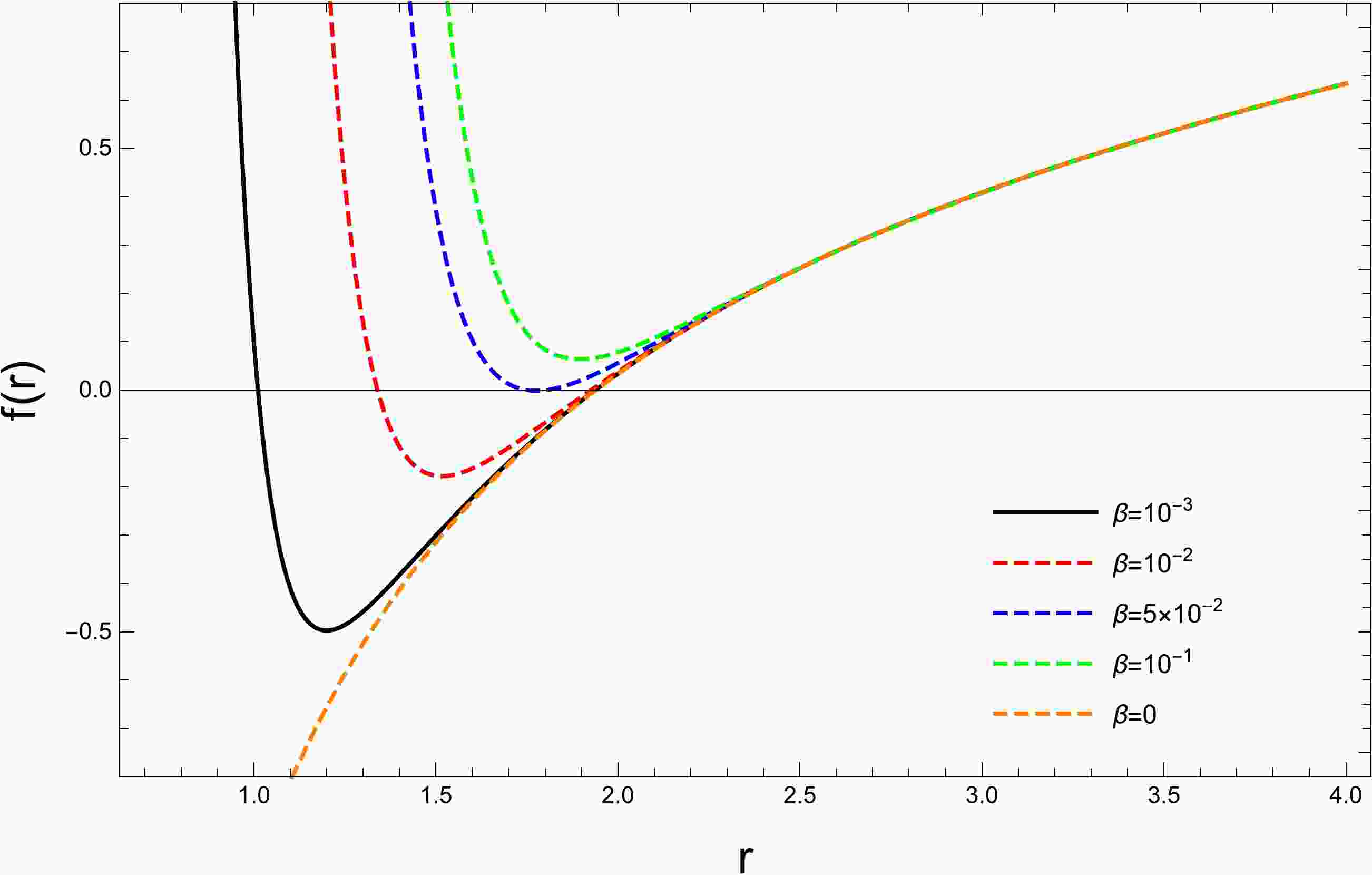
In black hole physics, the roots of the lapse function are used to determine the horizon of the black hole. In the problem under consideration, the coupling constant plays an important role in the values of the horizon and can be used to determine the critical value of the β parameter. To illustrate this, Fig. 1 shows the lapse function against the radial coordinate for various β parameter values.

Figure 1. (color online) Lapse function versus the radial coordinate for
$ m=1 $ and$ p=10^{-3} $ .Depending on the strength of the coupling constant, either two or no horizon can occur, and for a critical beta parameter value, only one horizon forms.
Now, let us focus on the derivation of the AdS black hole shadow in the context of EBR gravity. First, we consider the Lagrangian
$ \mathcal{L}=\frac{1}{2}g_{\mu \nu }\dot{x}^{\mu }\dot{x}^{\nu }=\frac{1}{2}\left[ -f\left( r\right) \dot{t}^{2}+\frac{1}{f\left( r\right) }\dot{r}^{2}+r^{2}\dot{\theta}^{2}+r^{2}\sin ^{2}\theta \dot{\phi}^{2}\right] , $

(6) where the dot represents the derivative with respect to the affine parameter τ, and
$ g_{\mu \nu } $ denotes the metric tensor. By implementing the Euler-Lagrange equation, we easily deduce the following constants of motion:$ \begin{aligned}[b] E=\;& \Bigg(1-\frac{2m}{r}+\frac{8\pi pr^{2}\left( 9-16384\pi ^{3}\beta p^{3}\right) }{27}+\frac{1664\beta m^{4}}{r^{10}}\\&+\frac{3072\pi \beta m^{3}p }{r^{7}}-\frac{576\beta m^{3}}{r^{9}} \\ &-\frac{40960\pi ^{2}\beta m^{2}p^{2}}{ 3r^{4}}-\frac{12288\pi \beta m^{2}p}{5r^{6}}\Bigg)\dot{t},\\[-10pt] \end{aligned} $

(7) $ P_{\phi }=L=r^{2}\sin ^{2}\theta \dot{\phi}. $

(8) Here, E and L represent the test particle's energy and angular momentum, respectively. The next step involves acquiring the geodesic form of the particle. This can be achieved using the Hamilton-Jacobi equation
$ \frac{\partial S}{\partial \tau }+H=0, $

(9) where S and H denote the Jacobi action and Hamiltonian, respectively.
$ H=\frac{1}{2}g^{\mu \nu }p_{\mu }p_{\nu }. $

(10) By following the relation between the Jacobi action and the momentum,
$ p_{\mu } $ ,$\frac{\partial S}{\partial x^{\mu }}=p_{\mu }, $

(11) and employing the separation method based on Carter constants [67],
$ S=\frac{\tilde{m}^{2}}{2}\tau -Et+L\phi +S_{\theta }\left( \theta \right) +S_{r}\left( r\right) , $

(12) we obtain
$ \begin{aligned}[b]& \frac{E^{2}}{f\left( r\right) }-f\left( r\right) \left( \frac{\partial S_{r} }{\partial r}\right) ^{2}-\frac{1}{r^{2}}\left( \frac{L^{2}}{\sin ^{2}\theta}+\mathcal{K-}L^{2}\cot ^{2}\theta \right)\\& -\frac{1}{r^{2}}\left( \left(\frac{\partial S_{\theta }}{\partial \theta }\right) ^{2}-\mathcal{K}+L^{2}\cot ^{2}\theta \right) =0. \end{aligned} $

(13) Here,
$ \mathcal{K} $ represents the Carter constant. It is worth emphasizing that the mass,$ \tilde{m} $ , must be equalized to zero because the considered particle is a photon. Next, we utilize the relations$ \dfrac{\partial S_{\theta }}{\partial \theta }=p_{\theta } $ and$ \dfrac{\partial S_{r}}{\partial r}=p_{r} $ and obtain$ \frac{\partial S_{\theta }}{\partial \theta }=r^{2}\frac{\partial \theta }{ \partial \tau }, $

(14) $ \frac{\partial S_{r}}{\partial r}=\frac{1}{f\left( r\right) }\frac{\partial r }{\partial \tau }. $

(15) By embedding Eqs. (14) and (15) into Eq. (13), we recast it as two separate equations:
$ r^{2}\left( \frac{\partial S_{r}}{\partial r}\right) ^{2}=r^{2}\frac{E^{2}}{ f^{2}\left( r\right) }-\frac{\left( L^{2}+\mathcal{K}\right) }{f\left( r\right) }, $

(16) $ \left( \frac{\partial S_{\theta }}{\partial \theta }\right) ^{2}=\mathcal{K} -L^{2}\cot ^{2}\theta . $

(17) Then, we use the canonically conjugate momentum definition to express the complete set of equations of motion
$ r^{2}\frac{\partial \theta }{\partial \tau }=\pm \sqrt{\Theta }\sqrt{ \mathcal{K}-L^{2}\cot ^{2}\theta }, $

(18) $ r^{2}\dot{r}=\pm \sqrt{\mathcal{R}}\sqrt{r^{4}E^{2}-r^{2}f\left( r\right) \left( L^{2}+\mathcal{K}\right) }, $

(19) where
$ \Theta = \mathcal{K}-L^{2}\cot ^{2}\theta , $

(20) and
$ \mathcal{R}\left( r\right) = r^{4}E^{2}-r^{2}f\left( r\right) \left( L^{2}+\mathcal{K}\right) . $

(21) Here, the symbols
$ "+" $ and$ "-" $ correspond to the motion of photons in the outgoing and ingoing radial directions, respectively.It is known that the presence of unstable null circular orbits could indicate the shadow boundary of black holes. To determine these orbits, we must re-express the radial null geodesic equation in the following manner:
$ \left( \frac{\partial r}{\partial \tau }\right) ^{2}+V_{\rm eff}\left( r\right) =0. $

(22) Here, the effective potential of the radial motion,
$ V_{\rm eff}\left(r\right) $ , reads as$ V_{eff}\left( r\right) =\frac{f\left( r\right) }{r^{2}}\left( L^{2}+\mathcal{ K}\right) -E^{2}. $

(23) It is important to mention that the resulting effective potential perfectly matches the Schwarzschild scenario in the zero limit of β and p. We believe it necessary to briefly investigate the behavior of the effective potential before obtaining the optical properties. To this end, Figs. 2 and 3 show plots of the effective potential function against radial distance for various values of the parameters m, p, and β.

Figure 2. (color online) Variation in the effective potential as a function of the radial coordinate for
$ \beta =0.01 $ ,$ L=5 $ ,$ \mathcal{K=}1 $ , and$ E=1. $ 
Figure 3. (color online) Variation in the effective potential with respect to distance r by considering different values of β. We use
$ p=0.05 $ ,$ L=5 $ ,$ \mathcal{K=}1 $ , and$ E=1. $ In particular, Fig. 2 demonstrates how the mass and the pressure affect the effective potential. The peaks in these graphs reveal the presence of unstable circular photon orbits. Here, we observe that the peaks shift to the left with decreasing values as the black hole mass increases for fixed values of β and p. In addition, when m remains fixed, the maxima also increase and shift to the left as the black hole pressure increases. Another important observation is that for several pressure values, that is,
$ p=10^{-3} $ and$ p=3\times 10^{-3} $ , the effective potential becomes negative for larger r values. These cases show that the test particle can have bound orbits; thus, it cannot reach infinity.Figure 3 presents the influence of the EBR parameter on the effective potential. With an increase in the EBR parameter, the peak value of the potential decreases significantly. However, we do not observe any impact of this parameter on the photon sphere size of the black hole because the peak position of the effective potential changes its position with respect to r.
Next, we impose the conditions [68]
$ \left. V_{\rm eff}\left( r\right) \right\vert _{r=r_{p}}=\left. \frac{{\rm d} V_{\rm eff}\left( r\right) }{{\rm d} r}\right\vert _{r=r_{p}}=0, $

(24) or
$ \left. \mathcal{R}\left( r\right) \right\vert _{r=r_{p}}=\left. \frac{ {\rm d}\mathcal{R}\left( r\right) }{{\rm d}r}\right\vert _{r=r_{p}}=0, $

(25) to identify the unstable circular orbits, where
$ r_{p} $ denotes the radius of the photon sphere. Using the set of equations given in Eqs. (24) and (25), we obtain the following formula$ \begin{aligned}[b] &2-\frac{6m}{{ r_p}}+\frac{19968\beta m^{4}}{{ r_p}^{10}}+\frac{576\beta m^{3}\left( 48\pi p{ r_p}^{2}-11\right) }{{ r_p}^{9}}\\&-\frac{16384\pi \beta m^{2}p\left( 25\pi p{ r_p}^{2}+6\right) }{5{ r_p}^{6}}=0, \end{aligned} $

(26) Alternatively, we must not forget the label
$ \begin{aligned}[b]& 2-\frac{6m}{{ r_p}}+ \beta \frac{64 m^2}{r_p^6}\Bigg[\frac{312m^2}{r_p^4}+\frac{9m}{r_p^3}\left( 48\pi p{ r_p}^{2}-11\right)\\&-\frac{256\pi p }{5} \left( 25\pi p{ r_p}^{2}+6\right)\Bigg]=0, \end{aligned} $

(27) and then, using the two impact parameter definitions
$ \zeta =\frac{L}{E}, \quad \quad \eta =\frac{\mathcal{K}}{E^{2}}, $

(28) we find
$ \eta +\zeta ^{2}=\frac{4r_{p}^{2}}{2f\left( r_{p}\right) + { r_p} f^{\prime }\left( r_{p}\right) }. $

(29) Note that Eq. (26) cannot be solved analytically; therefore, we use numerical methods. Because EBR gravity bears an extra parameter on the solutions, we must assign different values to β. Keeping this in mind, we obtain numerical solutions for the photon sphere radius and present the computed values of
$ \eta+\zeta ^{2} $ in Tables 1, 2, and 3.p $ m=1,\beta =0.01 $ 

$ m=0.5,\beta =0.01 $ 

$ r_{p} $ 

$ \eta +\zeta ^{2} $ 

$ r_{p} $ 

$ \eta +\zeta ^{2} $ 

$ 10^{-3} $ 

3.00058 22.0241 1.49757 6.42059 $ 3\times 10^{-3} $ 

3.00312 16.095 1.51222 5.83382 $ 5\times 10^{-3} $ 

3.00683 12.6838 1.52793 5.34949 $ 7\times 10^{-3} $ 

3.01169 10.4679 1.54447 4.94251 $ 9\times 10^{-3} $ 

3.01764 8.91302 1.56162 4.59533 Table 1. Values of photon radius
$ r_{p} $ and impact parameters$ \eta +\xi ^{2} $ for different values of pressure.m $ p=0.005,\beta =0.01 $ 

$ p=0.005,\beta =0.001 $ 

$ r_{p} $ 

$ \eta +\zeta ^{2} $ 

$ r_{p} $ 

$ \eta +\zeta ^{2} $ 

$ 0.1 $ 

0.695426 0.786735 0.531083 0.51896 $ 0.08 $ 

0.645059 0.648966 0.493188 0.418694 $ 0.06 $ 

0.585656 0.511668 0.448215 0.32319 $ 0.04 $ 

0.511282 0.371854 0.391641 0.229921 $ 0.02 $ 

0.405547 0.221649 0.310908 0.134011 Table 2. Values of photon radius
$ r_{p} $ and impact parameters$ \eta +\xi ^{2} $ for different values of black hole mass.β $ p=0.05,m=0.4 $ 

$ p=0.05,m=0.7 $ 

$ r_{p} $ 

$ \eta +\zeta ^{2} $ 

$ r_{p} $ 

$ \eta +\zeta ^{2} $ 

$ 10^{-3} $ 

1.30949 1.79214 2.15802 2.04302 $ 3\times 10^{-3} $ 

1.43968 1.79292 2.2522 2.08211 $ 5\times 10^{-3} $ 

1.52702 1.80692 2.32839 2.11966 $ 7\times 10^{-3} $ 

1.59474 1.82763 2.39318 2.15654 $ 9\times 10^{-3} $ 

1.65085 1.85168 2.44998 2.19322 Table 3. Values of photon radius
$ r_{p} $ and impact parameters$ \eta +\xi ^{2} $ for different values of β.In Ref. [69], the authors proposed the use of the celestial coordinates X and Y to visualize the shadow on the observer's frame. Following that suggestion, we employ the celestial coordinates defined as follows:
$ X=\lim\limits_{r_{o}\rightarrow \infty }\bigg(-r_{o}^{2}\sin \theta _{o}\frac{{\rm d}\phi }{{\rm d}r}\bigg), $

(30) $ Y=\lim\limits_{r_{o}\rightarrow \infty }\bigg(r_{o}^{2}\frac{{\rm d}\theta }{{\rm d}r}\bigg). $

(31) Here,
$ r_{0} $ and$ \theta _{o} $ represent the distance and angle between the shadow and the observer, respectively. In the case of the null geodesic, we obtain$ X=-\frac{\zeta }{\sin \theta _{o}}, $

(32) $ Y=\pm \sqrt{\eta -\zeta ^{2}\cot ^{2}\theta _{o}}. $

(33) Then, we consider the observer on the equatorial hyperplane and take
$ \theta _{o}=\pi /2 $ . Therefore, Eqs. (32) and (33) reduce to the following form:$ X=-\zeta , $

(34) $ Y=\pm \sqrt{\eta }. $

(35) Consequently, Eq. (29) becomes
$ X^{2}+Y^{2}=\eta +\zeta ^{2}=\frac{4r_{p}^{2}}{2f\left( r_{p}\right) +r_{p} f^{\prime }\left( r_{p}\right) }=R_{s}^{2}. $

(36) Using a serial expansion up to the first order of β, the shadow radius
$ R_{s} $ reads as$ \begin{aligned}[b]\\[-12pt] R_{s}^{2} =\frac{6r_{p}^{2}}{3r_{p}-3m+16\pi pr_{p}^{3}} +\frac{64\beta \left( 28080m^{4}-8505m^{3}r_{p}+32400\pi m^{3}pr_{p}^{3}-57600\pi ^{2}m^{2}p^{2}r_{p}^{6}-20736\pi m^{2}pr_{p}^{4}+40960\pi ^{4}p^{4}r_{p}^{12}\right) }{15r^{7}\left( 3r_{p}-3m+16\pi pr_{p}^{3}\right) ^{2}}. \,\,\,\,\, \end{aligned} $ 
(37) In Figs. 4−6, we illustrate the dependence of the shadow radius on the parameters p, m, and β.
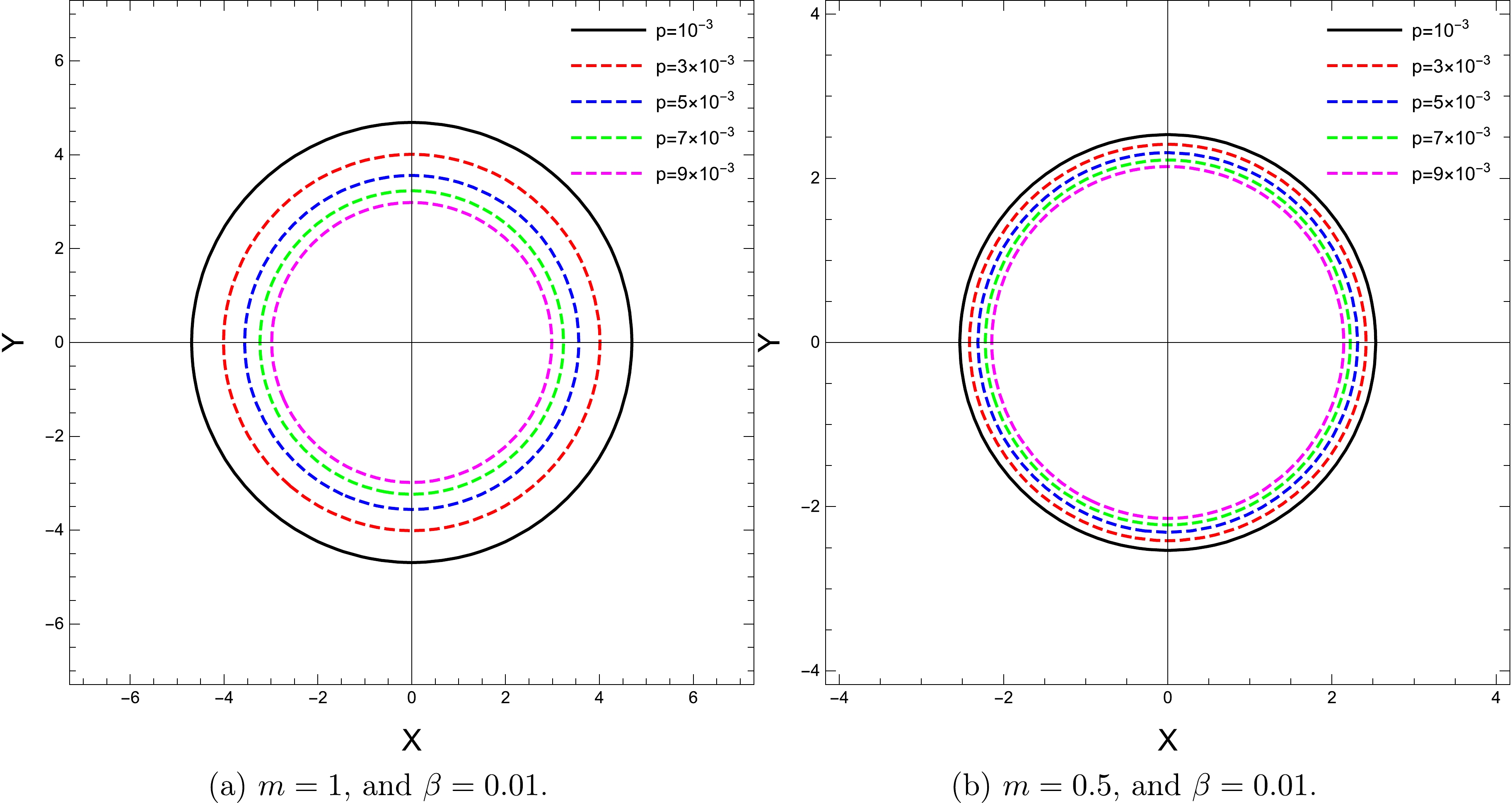
Figure 4. (color online) Impact of p on the shadow shape within the equatorial plane.

Figure 5. (color online) Impact of m on the shadow shape within the equatorial plane.
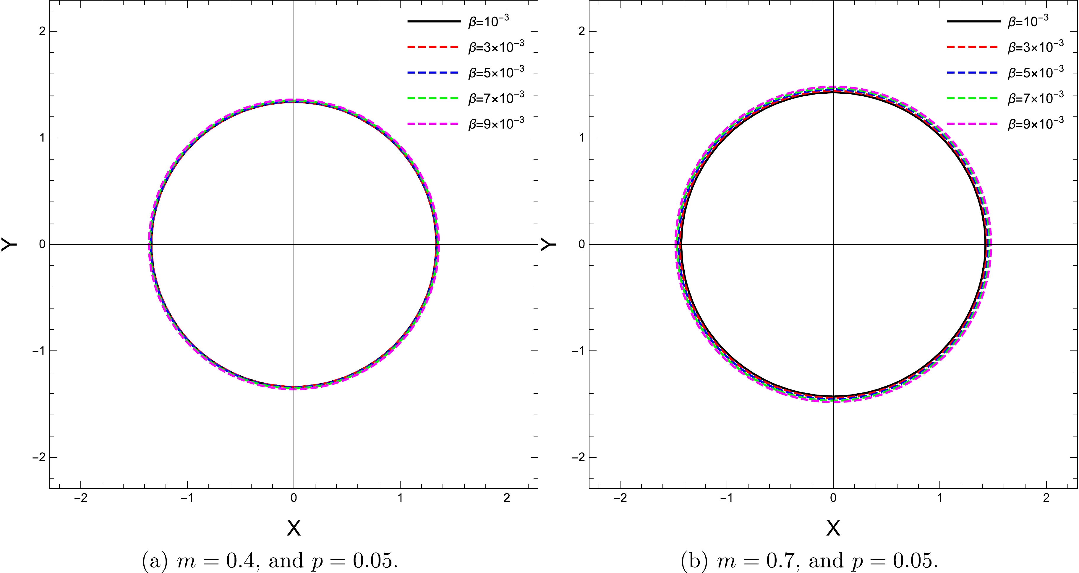
Figure 6. (color online) Impact of β on the shadow shape within the equatorial plane.
In particular, in Fig. 4, we show the stereographic projection of the shadow for different values of the black hole pressure. With an increase in the pressure, the radius of the black hole shadow decreases.
Subsequently, Fig. 5 shows that the increase in the mass of the black hole causes an increase in its shadow radius. Note that this characteristic change remains the same for different values of the β parameter.
Next, in Fig. 6, we observe the impact of the β parameter on the size of the black hole shadow. However, this effect seems to be relatively small compared with the impacts of other parameters. As the final visualization of this section, we present the close relationships between the shadow radius and the parameters in Fig. 7.
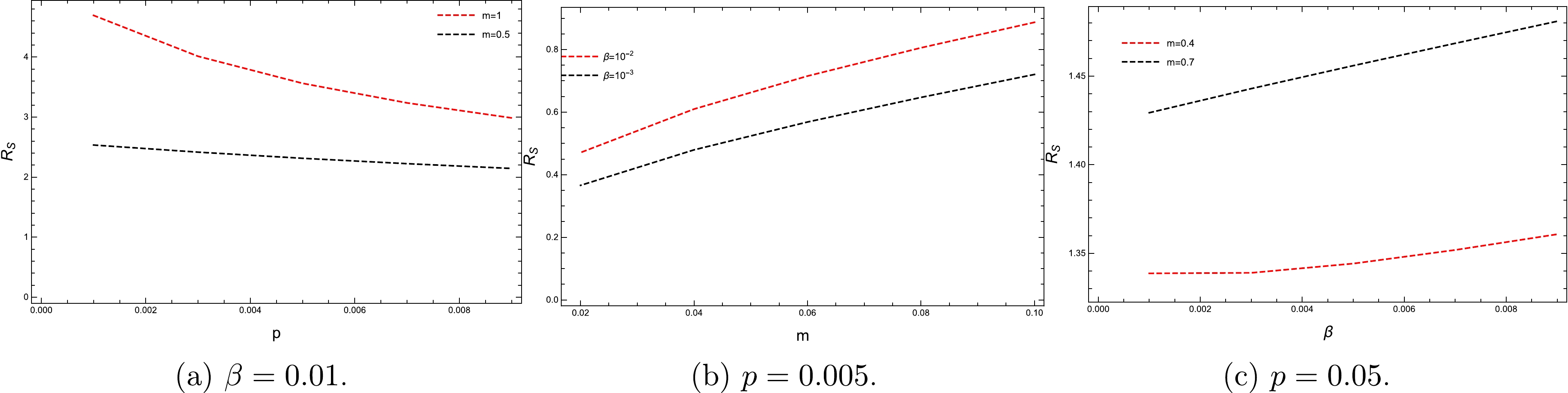
Figure 7. (color online) Correlation between the parameters and the shadow radius.
Now, we explore how the Event Horizon Telescope (EHT) measurements of M
$ 87^{\ast } $ [1] and Sgr.$ A^{\ast } $ [2] constrain the black hole parameters. To this end, we consider the necessary observational information listed in Table 4.Black hole Mass $/M\odot$ 

Angular diameter $\Theta /{\rm \mu as}$ 

Distance $/{\rm Mpc}$ 

Sgr. $ A^{\ast } $ 

$ \left(4.3\pm 0.013\right) 10^{6} $ 

$ \left(48.7\pm 7\right) $ 

$ \left(8.277\pm 0.033\right) 10^{-3} $ 

M $ 87^{\ast } $ 

$ \left(6.5\pm 0.90\right) 10^{9} $ 

$ \left(42.7\pm 3\right) $ 

$ 16.8 $ 

Table 4. Observational measurements of the Sgr.
$ A^{\ast } $ and M$ 87^{\ast } $ black holes.Using this data, it is possible to determine the diameter of the shadow image of Sgr.
$ A^{\ast } $ with$ d_{\text{Sgr.}A^{\ast }}=\frac{D\Theta }{M_{\text{Sgr.}A^{\ast }}}=\left( 9.5\pm 1.4\right) m, $

(38) where
$ d_{\text{Sgr.}A^{\ast }}=2R_{\text{Sgr.}A^{\ast }}. $ Thus, the radius of the observed shadow of Sgr.$ A^{\ast } $ in unit mass is$ R_{\text{Sgr.}A^{\ast }}=\left( 4.75\pm 0.70\right) m. $

(39) In the limit
$ p\rightarrow 0, $ the shadow radius reduces to$ R_{s}^{2}=\frac{6r_{p}^{2}}{3r_{p}-3m}+\frac{64\beta \left( 28080m^{4}-8505m^{3}r_{p}\right) }{15r^{7}\left( 3r_{p}-3m\right) ^{2}}. $

(40) Therefore, we can estimate the shadow radius of Sgr.
$ A^{\ast } $ and compare it with a Schwarzschild-like black hole in EBR gravity as presented in Table 5.β $ R_{s} $ 

$ 10^{-2} $ 

2.53637 $ 2\times 10^{-2} $ 

2.84698 $ 5\times 10^{-2} $ 

3.31671 $ 10^{-1} $ 

3.72288 $ 2\times 10^{-1} $ 

4.17879 $ 5\times 10^{-1} $ 

4.86826 Table 5. Shadow radius comparison of the Sgr.
$ A^{\ast } $ black hole with a Schwarzschild-like black hole in EBR gravity.The results given in Table 5 show that the radius of the black hole shadow increases with an increase in the value of the EBR gravity parameter.
As a final remark, we must note that other studies in literature argue that these observations may also be compatible with alternative models to the black hole scenario [70−72]. We refrain from giving further details on this here.
-
Black holes can emit radiation through the Hawking radiation process. Under high-energy conditions, the absorption cross-section typically fluctuates around a constant value known as
$ \sigma _{\lim } $ . For a very long distance observer, the absorption cross-section gradually approaches the region where the black hole shadow is formed [73]. For a nearly spherically symmetric black hole,$ \sigma _{\lim } $ is approximately assumed to be equal to the photon sphere area,$ \sigma _{\lim }\sim \pi R_{s}^{2}. $

(41) Thus, for the examined black hole, the complete form of the energy emission rate reads as
$ \frac{{\rm d}^{2}E\left( \omega \right) }{{\rm d}t\, {\rm d}\omega }=\frac{2\pi ^{2}\sigma _{\lim }}{{\rm e}^{\frac{\omega }{T_{H}}}-1}, $

(42) where ω and
$ T_{H} $ denote the frequency of the photon and Hawking temperature, respectively. In Fig. 8, we depict the black hole's energy emission rate as a function of photon frequency ω for various β values. Fig. 8 illustrates that as β increases, the peak of the energy emission rate shifts to lower frequencies.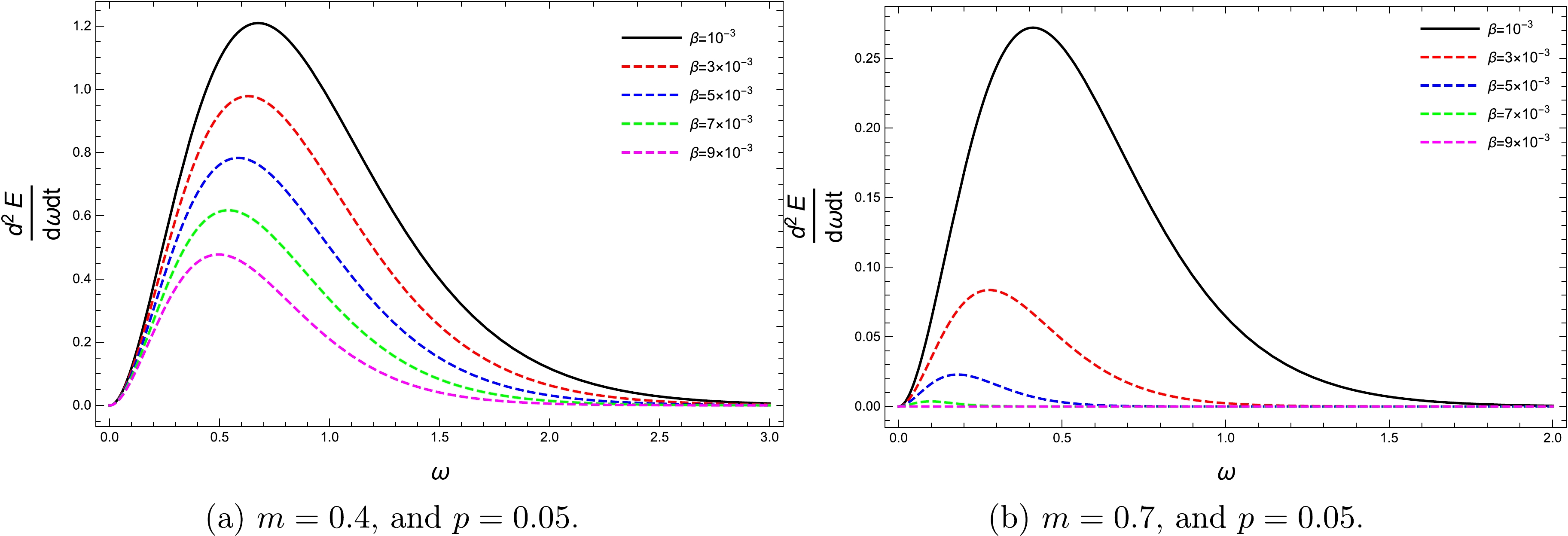
Figure 8. (color online) Energy emission rate behaviors of the EBR black hole for various values of the β parameter.
-
In this section, we aim to investigate how the plasma background affects the black hole shadow in EBR gravity. The main motivation for this is the idea that in most cases, black holes are surrounded by a medium that changes the geodesic of photons [24, 36]. We begin by considering a plasma with a refractive index
$ n=n\left(x^{i},\omega\right) $ , where ω denotes photon frequency. The existence of background plasma modifies the Hamiltonian by the extra terms that appear in the geodesic equations. Consequently, these modifications affect the trajectories of particles and present an explicit frequency dependence.Let us assume that the effective energy of the particles inside the plasma medium is [74]
$ \hbar \omega =p_{\alpha }u^{\alpha }, $

(43) and then we express the relationship between plasma frequency and the four-momentum of the photon as
$ n^{2}=1+\frac{p_{\alpha }p^{\alpha }}{\left( p_{\alpha }u^{\alpha }\right) ^{2}}. $

(44) Next, using the relationship between the refractive index and plasma frequency,
$ \omega _{p} $ , we express this as$ n^{2}=1-\left( \frac{\omega _{p}}{\omega }\right) ^{2}.$

(45) Then, we follow the authors of [75, 76] and use the radial power law form to express the refractive index of plasma as
$ n\left( r\right) =\sqrt{1-\frac{\rho }{r}}. $

(46) Here,
$ \rho \geq 0 $ is a constant. In the plasma background, the Hamilton-Jacobi equation becomes [74]$ \frac{\partial }{\partial \tau }S=-\frac{1}{2}\left[ g^{\mu \nu }p_{\mu}p_{\nu }-\left( n^{2}-1\right) \left( p_{0}\sqrt{-g^{00}}\right) ^{2}\right], $

(47) which leads to modifications in certain vacuum equations, including the equations of motion of photons. In particular, the new set of null-geodesic equations reads as
$ \dot{t}=\frac{n^{2}E}{f\left( r\right) }, $

(48) $ r^{2}\dot{r}=\sqrt{r^{4}n^{2}E^{2}-r^{2}f\left( r\right) \left( L^{2}+ \mathcal{K}\right) } , $

(49) $ r^{2}\dot{\theta}=\sqrt{\mathcal{K}-L^{2}\cot ^{2}\theta } , $

(50) $ L=r^{2}\sin ^{2}\theta \dot{\phi} . $

(51) In this case, the effective radial potential takes the form
$ \tilde{V}_{\rm eff}\left( r\right) =\frac{f\left( r\right) }{r^{2}}\left( L^{2}+ \mathcal{K}\right) -n^{2}E^{2}, $

(52) and in the absence of a plasma background, it reduces to Eq. (23). After repeating the same method given above, we obtain the unstable circular orbit conditions as
$ \left. \left( n\left( r\right) rf^{\prime }\left( r\right) -2n\left( r\right) f\left( r\right) -2rn^{\prime }\left( r\right) f\left( r\right) \right) \right\vert _{r=r_{p}}=0. $

(53) Then, using the impact parameters, we obtain
$ \eta +\zeta ^{2}=r_{p}^{2}\frac{n^{2}\left( r_{p}\right) }{f\left( r_{p}\right) }. $

(54) Using numerical methods, we compute the photon radius and
$ \eta+\zeta ^{2} $ for different values of$ \left(m,p,\beta \right) $ in the presence of the plasma background, and our results are shown in Tables 6, 7, and 8.p $ \rho =0.4 $ 

$ \rho =0.2 $ 

$ r_{p} $ 

$ \eta +\zeta ^{2} $ 

$ r_{p} $ 

$ \eta +\zeta ^{2} $ 

$ 10^{-3} $ 

2.9114 6.54089 2.95793 6.94591 $ 3\times 10^{-3} $ 

2.88369 4.82238 2.94543 5.0969 $ 5\times 10^{-3} $ 

2.85849 3.83137 2.93448 4.03125 $ 7\times 10^{-3} $ 

2.83575 3.18559 2.92506 3.33746 $ 9\times 10^{-3} $ 

2.81538 2.73075 2.91714 2.84935 Table 6. Computed values of photon radius and impact parameters with two different values of the plasma background parameter with
$ \beta =10^{-2} $ and$ m=1 $ .m $ \rho =0.4 $ 

$ \rho =0.2 $ 

$ r_{p} $ 

$ \eta +\zeta ^{2} $ 

$ r_{p} $ 

$ \eta +\zeta ^{2} $ 

$ 0.1 $ 

0.650461 0.450281 0.679367 0.789876 $ 0.08 $ 

0.599232 0.347518 0.629579 0.677837 $ 0.06 $ 

0.536295 0.234569 0.570532 0.559665 $ 0.04 $ 

0.446746 0.0873573 0.496155 0.428216 $ 0.02 $ 

/ / 0.389320 0.263556 Table 7. Computed values of photon radius and impact parameters with two different values of the plasma background parameter with
$ \beta =10^{-2} $ and$ p=0.005 $ .β $ \rho =0.4 $ 

$ \rho =0.2 $ 

$ r_{p} $ 

$ \eta +\zeta ^{2} $ 

$ r_{p} $ 

$ \eta +\zeta ^{2} $ 

$ 10^{-3} $ 

1.13057 0.939047 1.22393 1.09423 $ 3\times 10^{-3} $ 

1.27756 0.910117 1.36038 1.04595 $ 5\times 10^{-3} $ 

1.3702 0.897703 1.44959 1.02233 $ 7\times 10^{-3} $ 

1.44026 0.890983 1.51805 1.00805 $ 9\times 10^{-3} $ 

1.49761 0.863585 1.5745 0.998692 Table 8. Computed values of photon radius and impact parameters with two different values of the plasma background parameter with
$ m=0.4 $ and$ p=5\times 10^{-2} $ .Next, we use the celestial coordinates
$ Y=\pm \sqrt{\eta }, $

(55) $ X=-\zeta , $

(56) and we rewrite the square of the shadow radius in the presence of a plasma background as follows:
$ X^{2}+Y^{2}=\zeta ^{2}+\eta =r_{p}^{2}\frac{n^{2}\left( r_{p}\right) }{ f\left( r_{p}\right) }=R_{s}^{2}. $

(57) Finally, we demonstrate the dependence of the shadow radius,
$ R_{s} $ , on the parameters p, m, and β and the plasma parameters in Figs. 9−11.
Figure 9. (color online) Shapes of the black hole shadow in the equatorial plane by considering distinct values of p for two different values of the plasma medium and
$ m=1 $ ,$ \beta =10^{-2}. $ 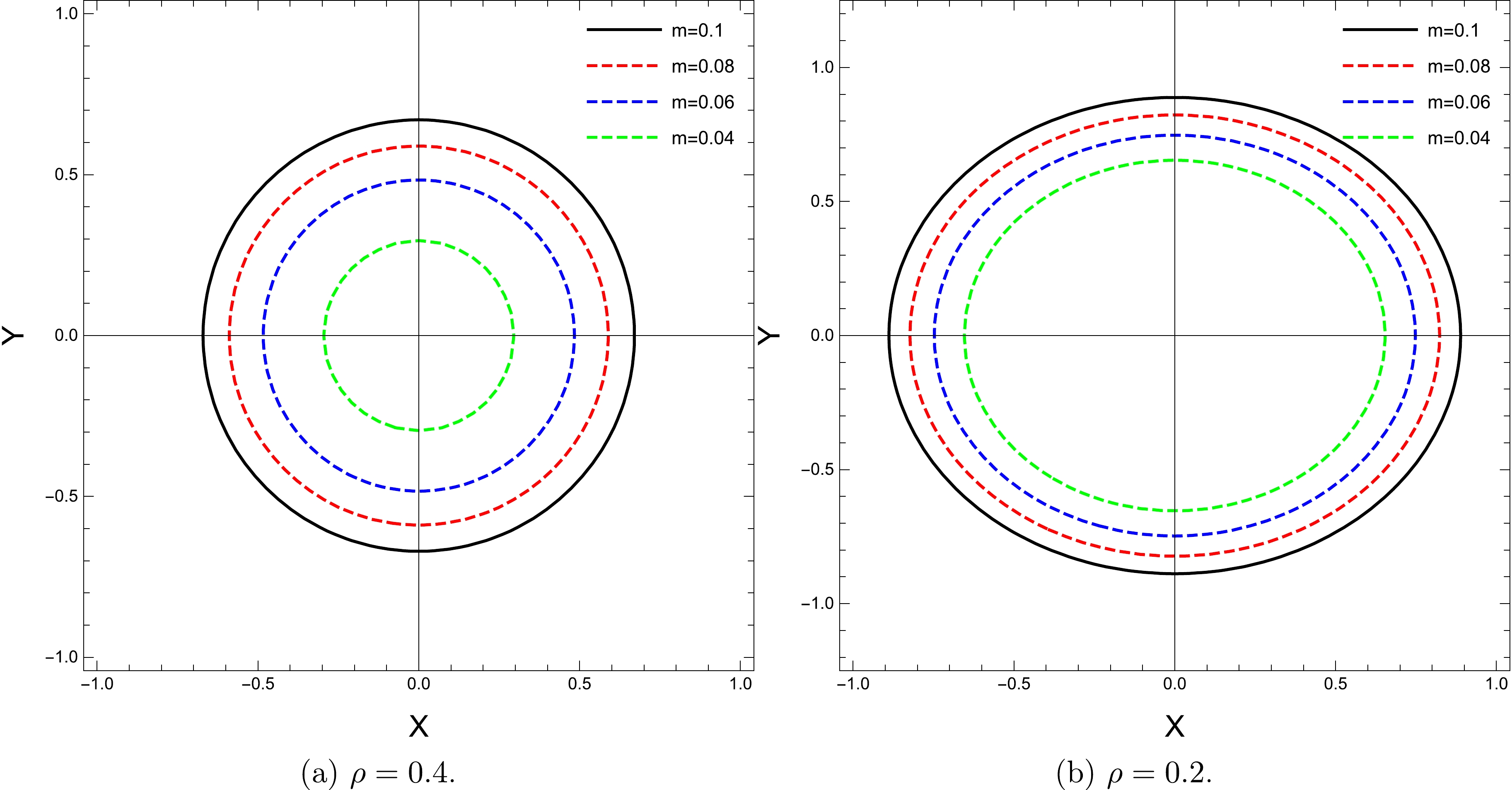
Figure 10. (color online) Shapes of the black hole shadow in the equatorial plane by considering distinct values of m for two different values of the plasma medium and
$ p=5\times 10^{-3} $ ,$ \beta =10^{-2}. $ 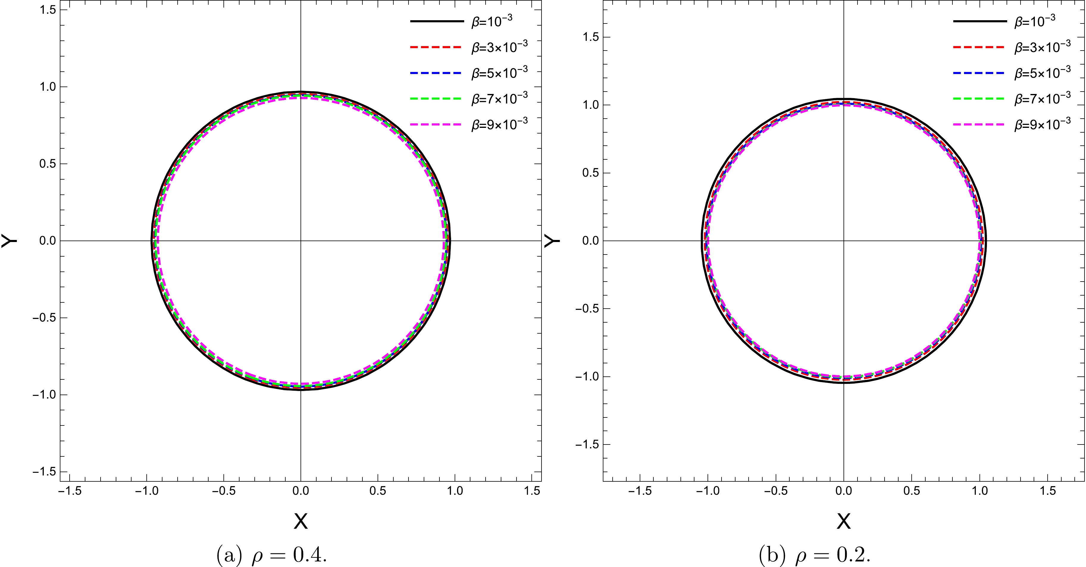
Figure 11. (color online) Shapes of the black hole shadow in the equatorial plane by considering distinct values of β for two different values of the plasma medium and
$ p=5\times 10^{-2} $ ,$ m=0.4 $ . -
In this study, we investigate AdS black hole shadows in EBR gravity by considering the AdS black hole solutions recently obtained by Sajadi et al. using perturbative analytic methods. After briefly discussing how they found the line element in four-dimensional EBR gravity, we derive constants of motion from the Euler-Lagrange equation and then use the Hamilton-Jacobi equation to find the null-geodesic equations of motion. Using the separation method, we obtain the factorized relations and express the effective potential. Next, we recall the conditions for unstable null circular orbits and obtain the photon sphere radius. For arbitrary values of mass, pressure, and EBR gravity coupling constants, we calculate the radii, and accordingly, depict the shadows. We find that an increase in pressure decreases the shadow radius, whereas an increase in black hole mass increases the radius. Moreover, we note that for higher values of the gravity coupling constant, the shadow radius increases; however, this impact is relatively smaller than the others. Next, we study the energy emission rate and find that an increase in the gravity coupling constant changes the peak value of the energy emission rate. Finally, we recalculate the geometry of AdS black hole shadows in the presence of a plasma background.
-
The authors are grateful to the anonymous reviewer for constructive comments.
-
The authors declare that the data supporting the findings of this study are available within the article.
Black hole shadows in Einstein-Bel-Robinson gravity
- Received Date: 2023-11-21
- Available Online: 2024-05-15
Abstract: Gravity models given by higher-order scalar curvature corrections are believed to bear important consequences. Einstein-Bel-Robinson (EBR) gravity with quartic curvature modification motivated Sajadi et al. to explore static spherically symmetric black hole solutions using perturbative methods. In this study, inspired by their work, we investigate AdS black hole shadows in EBR gravity and demonstrate how the gravity parameter alters the energy emission rate. Finally, we address the same problem in the presence of plasma, because the black holes are thought to be surrounded by a medium that changes the geodesic of photons.


 DownLoad: