


 Abstract
 HTML
HTML Reference
 Related
 PDF
PDF


-
The neutrinoless double beta decay (0νββ) experiment is currently the only practical experimental method to test the Majorana nature of neutrinos. Even after 75 years of experimental searches since the first attempt in 1948 [1], only null results have been obtained. Stringent limits are set for isotopes, for instance,
$ T_{1/2}>2.6 \times 10^{26} $ yr for 136Xe from the KamLAND-Zen experiment [2] and$ T_{1/2}>1.8 \times 10^{26} $ yr for 82Se from the GERDA experiment [3] at a 90% C.L.The next generation 0νββ experiments are aiming to obtain a half-life sensitivity of up to
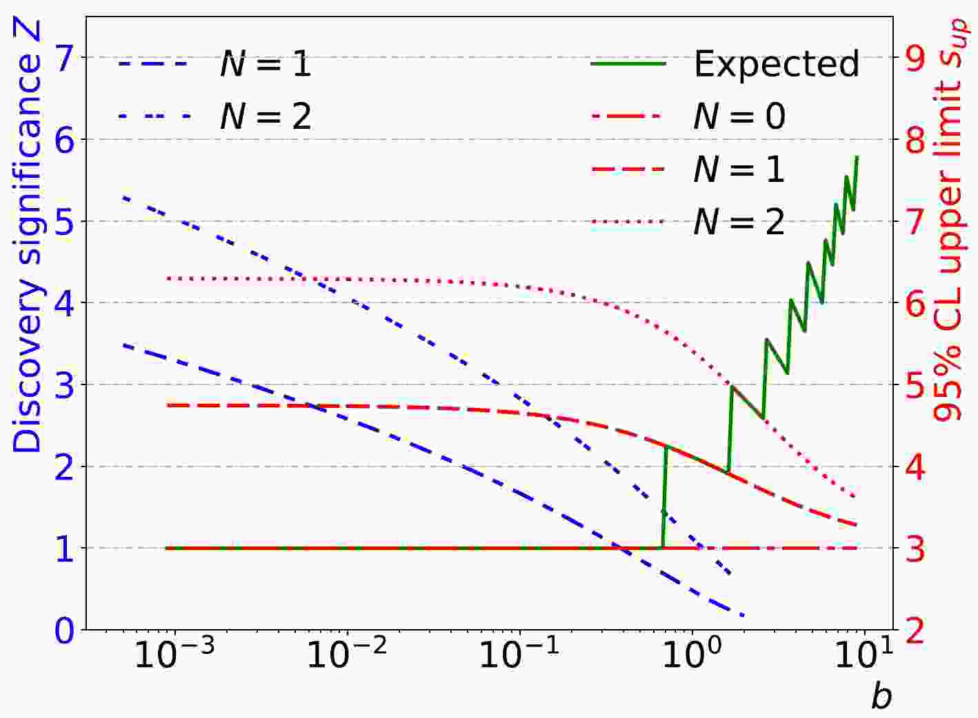
$ T_{1/2} \sim 10^{27} -10^{28} $ yr, corresponding to the effective Majorana mass$ m_{\beta \beta} \sim 5- $ 20 meV, below the Inverted Mass Ordering region.For this type of rare decay processes, background control is crucial. Ideally, experiments would like to achieve "zero background" to maximize the use of the isotopes, which are usually expensive. For a simple counting experiment, the dependence of sensitivity on the expected number of background events, b, is illustrated in Fig. 1. The 95% upper limit is calculated using the Bayesian statistics with a flat prior for signal. Moreover, the discovery significance is calculated following the frequentist definition [4, 5]. The expected limits become almost flat when
$ b<0.7 $ . However, the discovery could be considered as background free if$ b<0.0027 $ , below which one can claim a "$ 3\sigma $ significance" with a single event being observed. If$ b<0.0011 $ , an experiment could reach a "$ 5\sigma $ significance" with two observed events. To claim a "$ 5\sigma $ significance" with one observed event, one needs$ b<5.7 \times 10^{-7} $ . Keeping the background low is essential for early discovery of a signal if it exists.
Figure 1. (color online) Discovery significance Z and upper limit
$ s_{\rm{up}} $ at 95% C.L. as functions of b for the cases of zero, one, two, or more events (N) observed in the Region of Interest (ROI). The green solid line depicts the expected limit using the Asimov dataset (median of possible number of observed data).The two neutrino double beta decay (2νββ) is an intrinsic background that could only be reduced by improving the energy resolution. Other backgrounds come from the cosmic rays and the natural radioactivity in the environment, detector, and working medium. While most of these backgrounds could be suppressed by radio-purity material selection, shielding, or coincidence detection, the neutrino background, due to its weak interaction with materials, could survive and become an important background. As its contribution scales with the medium, it becomes particularly important for large detectors, which is the case for most of the next-generation experiments. Solar neutrino is the main source of the background in the relevant energy range (a few MeV).
Among the many technologies exploited by the next generation experiments, the high-pressure gaseous Time Projection Chamber (TPC) method has its unique advantages and is developing rapidly. High-pressure gaseous TPCs using 136Xe are explored by NEXT [6] and PandaX-III [7]. The use of 82SeF6 has been discussed in [8, 9], and a dedicated experiment is proposed in [10]. A few advantages make this experimental framework promising: 1) the high
$ Q_{\beta \beta} $ value of 82Se is above the energy of major radioactive gammas, 2) the low diffusion from the ion drifting allows good tracking, 3) the low noise pixel readout chips could provide excellent energy resolution, and 4) the deep Jingping underground Lab effectively reduces the cosmic background.Moreover, as the solar neutrino becomes an important background for 0νββ experiments, these experiments could facilitate solar neutrino studies. Both 82Se and 19F have been proposed for solar neutrino studies [11−16]. In the meantime, an electronegative gaseous TPC with high Fluorine content is also proposed for Dark Matter searches [17−19].
The focus of this study is to investigate the solar neutrino background for a high-pressure TPC using 82SeF6. Previous studies show that, for 82Se the single-beta decay events induced by the solar neutrino contribute 4.42 events/(ton·yr) in a 60 keV Region of Interest (ROI) window [20]. This value is large compared with that from the 2νββ process (0.15 events/(ton·yr)). This is because of the low interaction threshold (
$ Q_\nu = 172 $ keV) for inverse beta decay of 82Se to 82Br. For TPC detectors, these backgrounds would have signatures that differ with respect to the signal and thus could be reduced using the tracking information. In this study, we use simulations to assess the signatures of various backgrounds and the rejection capability. A better understanding of these backgrounds would help the sensitivity estimation and design optimization of future projects.The remainder of this paper is organized as follows. In Section II, we briefly describe the solar neutrino model and simulation setup of this study. We discuss each possible background source in Section III. Finally, we present our conclusions in Section IV.
-
The neutrino flux data from the Standard Solar Model with low metallicity (B16-AGSS09, [21]) are used as a baseline. The energy spectra are shown in Fig. 2 (left). The differences between this model and other models [22, 23] are quite small; the model dependence of our results will be discussed later. To calcualte the survival probability, Eqn. (2.8) presented in [24] and the latest neutrino oscillation parameters from NuFit [25, 26] are used. The value
$ N_e=100\; N_{\rm{A}}/{\rm{cm}}^3 $ is used to denote the electron density in the Sun, where$ N_{\rm{A}} $ is the Avogadro constant. When considering the matter effect on Earth, the day-night difference is calculated using Eqn. (2.21) presented in [24]. As shown in Fig. 2(right), the values are generally smaller than those in [27]. Because the difference between day and night is small in the low energy region, the day-night average is used in this study. The resulting spectra of$ \nu_e $ and$ \nu_{\mu, \tau} $ on Earth are also shown in Fig. 2 (left).
Figure 2. (color online) Energy spectra of the solar neutrino (left) and electron neutrino survival probability as a function of its energy (right). The continuous energy spectra of various neutrino production processes are stacked. The neutrino from 8Be and pep are drawn separately (in unit of cm-2s-1). The continuous spectra of
$ \nu_e $ and$ \nu_{\mu, \tau} $ on Earth are also shown using$ P_{ee} $ in the right figure. In the$ P_{ee} $ distribution, the red dash curve shows the function used in [27]. The two horizontal dash lines show the$ P_{ee} $ without matter effect on top and two flavour mixing limit on bottom. The green band shows the uncertainty from the$ 1\sigma $ variation of the oscillation parameters. -
Signal and background processes are simulated using Geant4 (version 11.1.2) [28−30]. The
${\mathrm{Bearden}}$ data are used for determining the binding energies to obtain more accurate X-ray fluorescence lines. A detector with dimensions 40 m × 40 m × 40 m is built and filled with 82SeF6 at$ 20^\circ{\rm{C}} $ temperature and 10 bar pressure. 100% enrichment of 82Se is used for simplicity. Events are generated with their primary interaction points uniformly distributed in a 0.5 m × 0.5 m × 0.5 m cube around the center. Signal events are generated using the${\mathrm{BxDecay0}}$ package (version 1.1.0) [31]. For various neutrino background events, particle guns are used to emit electrons or ions. For the detection, we consider a hexagon grid readout plane with pitch size 8 mm as suggested in [9]. The maximum step size is set at 1 mm to obtain a fine segmentation of the tracks.The simulation is divided into two parts. In the first part, the interactions of the final state particles of each process in the detector are simulated using Geant4. The steps that have non-zero energy deposition are recorded as "hits." In the second part, the energy of each step is converted to the number of electrons using the W-value, and assigned to pixels on the readout plane based on their location. As there is no measurement of the W-value for 82SeF6 available, the value
$ W=32 $ eV of the structurally similar SeF6 gas is used to obtain the number of ion pairs. Based on the discussion presented in [8], a 0.34% FWHM smear of total energy is introduced to account for the Fano factor. To consider the diffusion of the track during the drift, the$ x-y $ position of the ions are smeared using a Gaussian function having a 1 mm FWHM width. Existing studies and measurements suggest that this is achievable for a 1 m drift distance of ions by applying an electric field of approximately 65 kV/m [17, 32]. No smearing in the z direction is applied because the smear in the z direction also depends on the readout electronics, which has little impact to this study. In the second part, for efficient computing, the size of the detector is reduced to 7 m × 7 m in the$ x-y $ directions, a size that is already much larger than that of any planned detectors.In the event building, the signal in each pixel is divided into "blocks" based on the z profile of the signal. "Raw blocks" are built first based on the distance of the hits to their nearest neighbouring hits. If the distance is greater than 2 mm, they are added in two separate "raw blocks." The long "raw blocks" are divided into "blocks." If the length of a raw block in the z direction is greater than 8 mm, it is divided into several "blocks" with equal length, with the number of blocks being minimal. This division in the z direction, although having little impact on the results given in this paper, would facilitate other background studies to check the
$ {\rm{d}}E/{\rm{d}}x $ for particle identification and use the Bragg peak feature to separate the signal and single-electron background, even if the track is along the z direction and contained in a single pixel. Adjacent blocks are further merged to form a "cluster." Regarding the energy of each block, a further smear corresponding to 40$ e^- $ is applied to consider the uncertainty rising from recombination, readout electronics, and other effects. This yields an overall energy resolution of 1%.Figure 3 shows the 3D "hits" of each step and 2D projection of the "blocks" after the reconstruction for one typical signal event. One can clearly see the larger energy depositions (Bragg peaks) at both ends of the track.
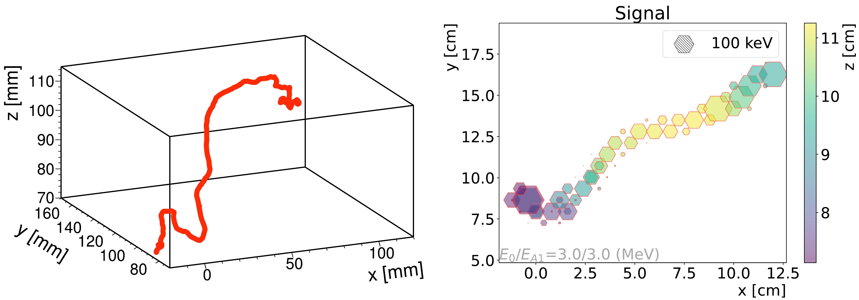
Figure 3. (color online) 3D "hits" obtained in the Geant4 simulation (left) and 2D projection of the "blocks" after the reconstruction (right) for a signal event. In the 2D view, the energy deposited in each pixel is represented by the size of the hexagon. The size corresponding to 100 keV energy is shown in the legend. The z coordinate is represented by the color of the filled hexagon. The blocks with the same edge color belongs to the same cluster. For the leading and sub-leading clusters, red and blue are used for the edges. The text in the bottom left corner gives the energy of the leading cluster (
$ E_0 $ ) and total energy ($ E_{AN} $ , where N is the number of clusters in the event). In this event, all blocks are collected in a single cluster. -
The neutrino could interact with the electrons or the 82Se and 19F nuclei. For electron-neutrino scattering (ES), the interaction is relatively simple, whereas for the interaction with nuclei, the subsequent decay of the nuclei in the final state could also mimic our signal and thus needs to be considered. Figure 4 illustrates the related interactions with the 82Se and 19F nuclei. 82Se could be converted to the
$ 1^+ $ excited state of 82Br via a Charge Current (CC) interaction with the neutrino. The excited state of 82Br decays to the isomer state 82mBr ($ J^\pi=2^- $ ) via gamma radiation. Subsequently, 82mBr could decay to the ground state by radiating a 46 keV gamma with a 97.6% branching fraction or proceed with a$ \beta^- $ decay to 82Kr directly with a 2.4% branching fraction. 82mBr has a large probability (88%) to decay to the ground state of 82Kr. In contrast, the decay of ground state 82Br to the ground state of 82Kr is forbidden. Thus, it decays to the excited states of 82Kr, which subsequently decays to the ground state of 82Kr, radiating multiple gammas. The picture for 19F is simple, as in the CC interaction it would transit to the ground state of 19Ne, which in turn decays back to 19F via$ \beta^+ $ decay. Two 0.511 MeV gammas are produced from the positron-electron annihilation.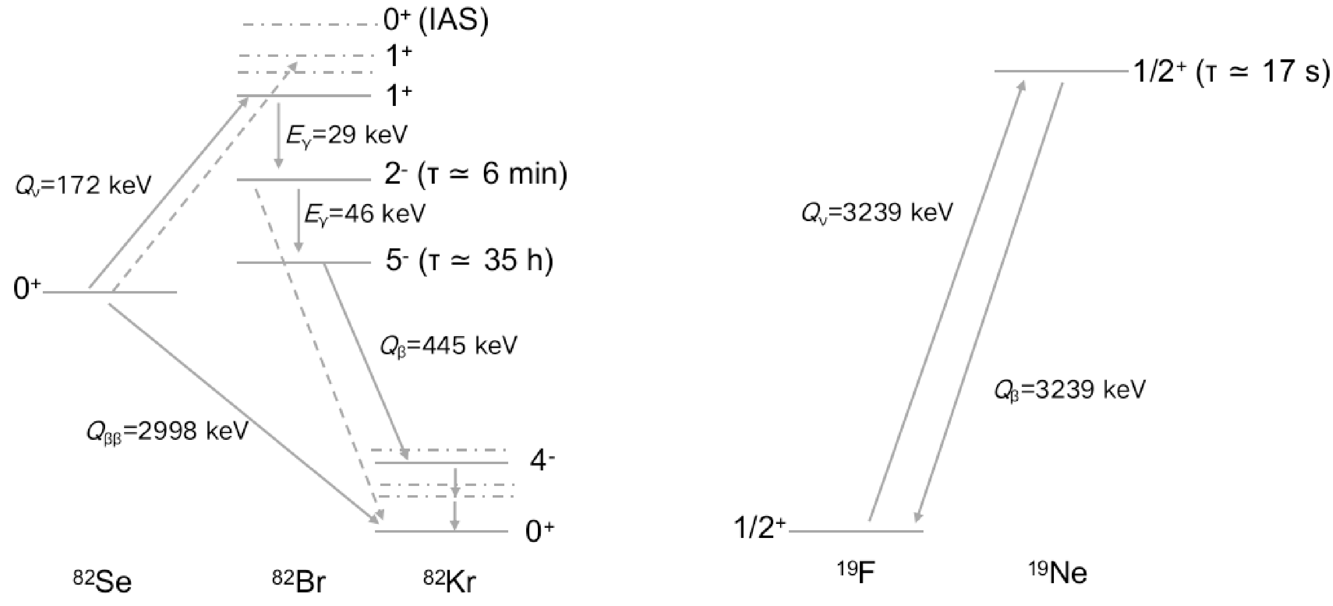
Figure 4. Schematics of the interactions for 82Se (left) and 19F (right). The most relevant levels and transitions are shown as solid lines. The less relevant levels are shown as dash-dot lines, and the transitions having small contributions are shown as dash lines.
Figure 5 shows the energy spread (the largest distance between the interaction point and the location of any energy deposition, L) and number of reconstructed clusters in these processes. Signal events typically have a spread
$ L \sim 10\;{\rm{cm}} $ , but there is a long tail on the large L side due to bremsstrahlung gammas. The 82Br (g.s.) and 19Ne decays have a much larger energy spread and more clusters than other processes because of the production of high energy gammas. The distribution of the energy of the reconstructed clusters for each process is shown in Fig. 6. As expected, the signal events peak at$ Q_{\beta \beta} $ region, but there also exists a significant fraction of events having low energy clusters. They are again mainly due to the bremsstrahlung gammas. The various background processes are discussed in detail in the following subsections.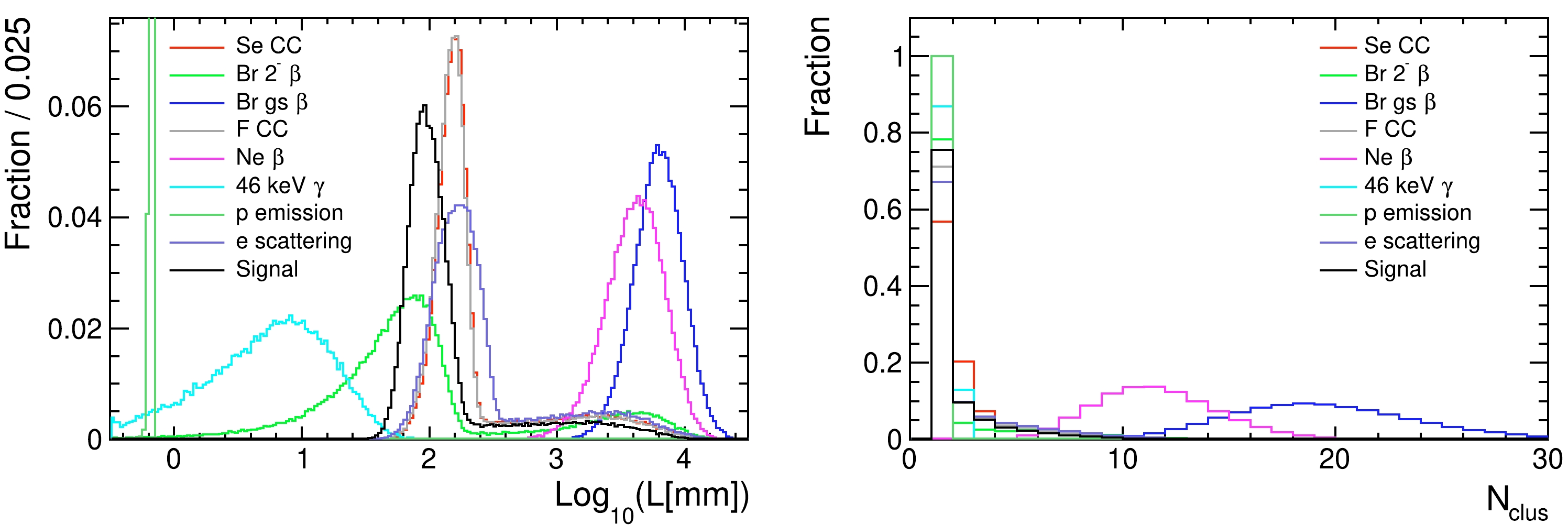
Figure 5. (color online) Furtherest energy deposition from the interaction point (left) and the number of reconstructed clusters (right) for various processes.
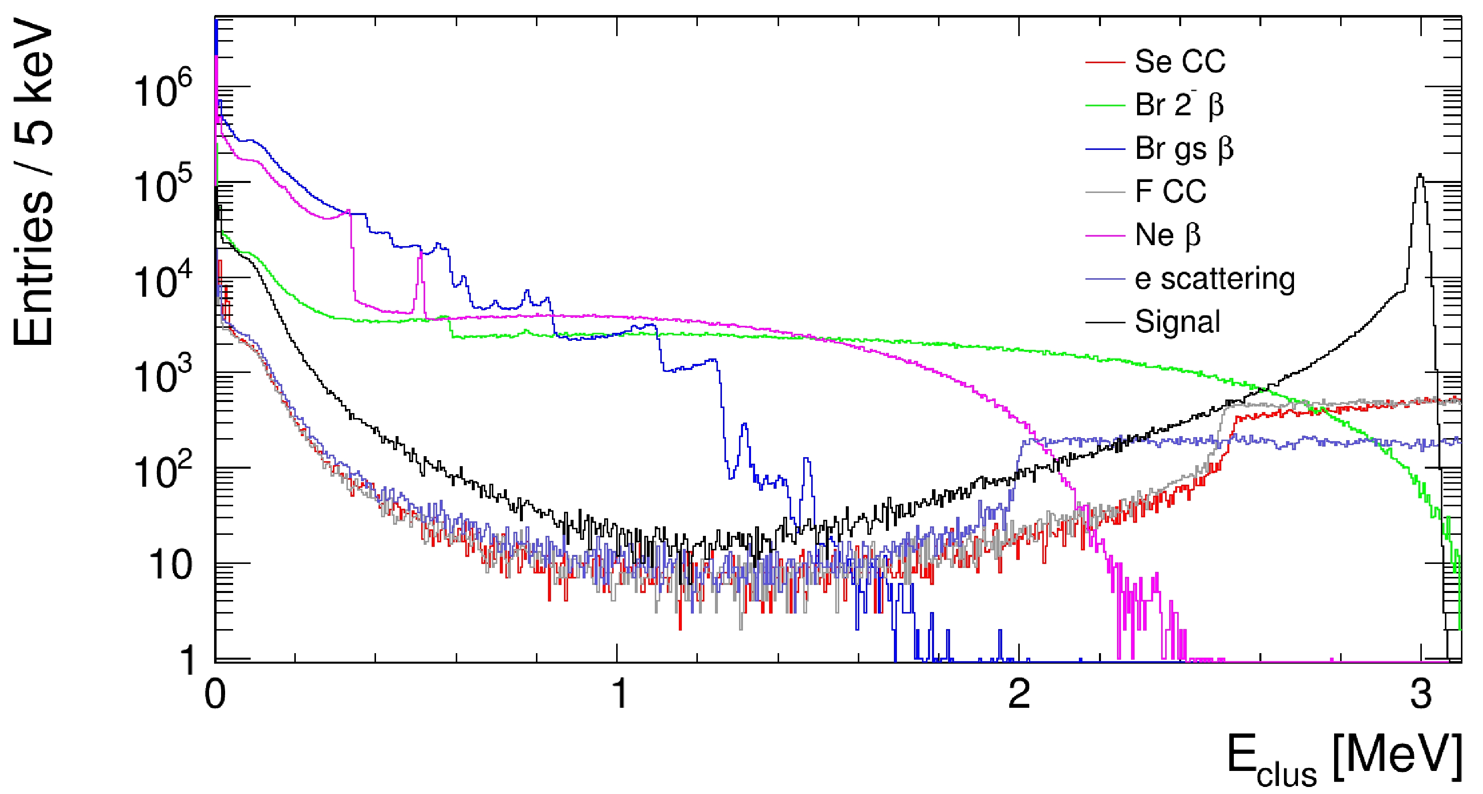
Figure 6. (color online) Distribution of the energy of the clusters. For Se CC, F CC, and ES processes, only the events that are in the energy window are simulated. Thus, the step structure occurs at 2 MeV for ES and approximately 2.5 MeV for Se CC and F CC. For other processes, the full spectra are used. 1M events are generated for Br decay, Ne decay, and signal events, and 100k events are generated for other processes.
-
All three flavors of neutrinos could exhibit neutral current (NC) interactions with electrons; in addition, for electron neutrino, CC interaction could also happen. These processes are widely utilized in the solar neutrino studies [33−36]. As possible backgrounds for neutrinoless double beta decay search, they have been studied for Ge [37] and other isotopes [38]. The differential cross-section for a neutrino with energy
$ E_\nu $ is [39, 40]$ \frac{{\rm{d}}\sigma}{{\rm{d}}T} = \frac{2G_{\rm F}^2 m_{\rm{e}}}{\pi}\left[g_L^2 + g_R^2\left(1-\frac{T}{E_\nu}\right)^2-g_{L} g_{R}\frac{m_{\rm{e}} T}{E_\nu^2}\right], $

(1) where T is the kinetic energy of the outgoing electron,
$G_{\rm F}$ is the Fermi constant,$ g_L=\sin^2\theta_{\rm{W}}\pm\dfrac{1}{2} $ (the upper sign is for$ \nu_e $ and lower sign for$ \nu_\mu $ and$ \nu_\tau $ ) and$ g_R=\sin^2\theta_{\rm{W}} $ are the coupling parameters, and$ \theta_{\rm{W}} $ is the Weinberg angle. The maximum value that T could reach is$T_{\rm{max}}= \dfrac{2E_\nu^2}{m_{\rm{e}}+2E_\nu}$ . The angle between the electron and neutrino momenta, θ, is given by$ \cos^2\theta = \frac{T(m_{\rm{e}}+E_\nu)^2}{(T+2m_{\rm{e}})E_\nu^2}. $

(2) For simplicity, the radiative correction leading up to a 4% reduction [41] of the cross-section is not included, as the effect is much smaller than the uncertainty arising from the neutrino flux.
Figure 7 (left) shows the energy spectrum of electron. The contribution from
$ \nu_{\mu, \tau} $ is approximately 0.22, including the effect from oscillation and the difference in cross-sections. The total event rate is 481.0 events/(ton·yr); however, the vast majority of the recoil electrons have a low energy from the pp neutrinos. The event rate drops by four orders of magnitude between the pp neutrino region and ROI at approximately 3 MeV. The estimate is 0.00445 events/(30 keV ton·yr) near the ROI, with a relative uncertainty of 12% from the neutrino flux, consistent with the results obtained by scaling the numbers presented in [38].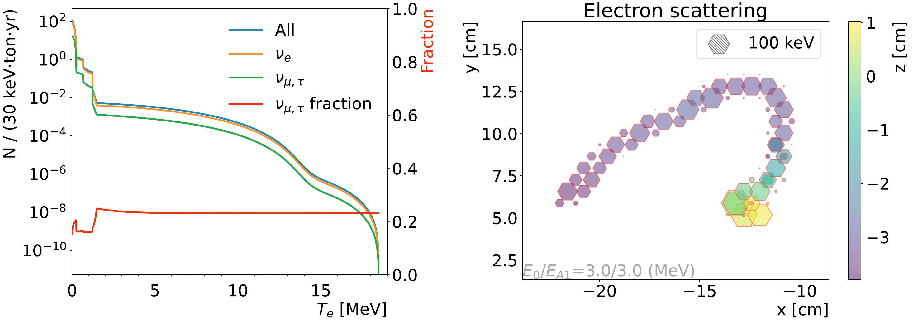
Figure 7. (color online) Energy spectra of the outgoing electron (left) and the event display of one typical ES event (right).
The signatures of this type of events are the same as those of the single electron events occurring due to natural radioactive decays. 100k ES events with
$ 2<T< 5 \;{\rm{MeV}} $ are simulated. Observe from Fig. 5(left) that the distribution of the spread is similar to signal events, but the mean is larger. The wider distribution is due to the large energy range. Moreover, these events have a small number of clusters. A typical event is shown in Fig. 7 (right). The algorithms developed to distinguish the radioactive decay background could also be used to reject this background. Machine learning methods show promising results in this domain [7, 8, 42, 43].As there is a strong correlation between the neutrino momentum direction and outgoing electron momentum direction, the angular information might also help the signal/background classification. Figure 8 plots the cosine value of the zenith angle. It peaks at
$ \cos\theta \sim 0.9 $ , corresponding to$ \theta \sim 25^\circ $ , which is expected because the majority of the electrons are from the interaction of the 8B neutrino that peaks at approximately 6 MeV in the energy distribution. Track direction determination similar to that implemented in [44] could be used to extract the angle. While a selection based on the angles would always bring inefficiency for signal classification, alternatively, the angular variables could be added in the machine learning methods to provide extra information.
Figure 8. (color online)
$ \cos\theta-T $ distribution for electrons in the range$ 2<T<5 $ MeV (left). The distribution of$ \cos\theta $ for electron scattering events with$ |T-Q_{\beta \beta}|<30 $ keV (right). -
As transition to the ground state of 82Br is forbidden, when interacting with the solar neutrino, the 82Se could undergo an inverse beta decay to the excited states of 82Br,
$ \nu_e + ^{82}{\rm{Se}} \to e^- + ^{82}{\rm{Br}}^* , $

(3) and
$ ^{82}{\rm{Br}}^* $ will mainly remain in the$ 1^+ $ Gamow-Teller (GT) states. The lowest of such a state is the 75 keV excitation energy state. The threshold of this process is$ Q_\nu = 172 $ keV. The final state electron will have energy$ E=E_\nu-Q_\nu $ . Transition to the$ 0^+ $ Isobaric Analog State (IAS) is also possible for high energy neutrinos, but it is suppressed by the low neutrino flux due to the high threshold$ Q_\nu = 9.673 $ MeV.The cross-section for the transition to the excited state k is [45]
$ \begin{aligned}[b] \sigma_k =\;& \frac{G_F^2\cos^2\theta_c}{\pi} p_e E_e F(Z, E_e)\left[ B(F)_k + \left(\frac{g_A}{g_V}\right)^2 B(GT)_k\right] \\ =\;& (1.597 \times 10^{-44}\; {\rm{cm}}^2)p_e E_e F(Z, E_e)\\&\times\left[ B(F)_k + \left(\frac{g_A}{g_V}\right)^2 B(GT)_k\right], \end{aligned} $

(4) where
$ \theta_c $ is the Cabibo angle,$ p_e $ ($ E_e $ ) is the outgoing electron momentum (total energy), and$ F(Z, E_e) $ is the Fermi function. In this section, only the transition to the GT states is considered, leaving the discussion of IAS to Section III.E. For these GT states, the Fermi response$ B(F)=0 $ , and the values of Gamow-Teller response,$ B(GT) $ , for each GT states are taken from [14], following the same configuration: individual resonances are used for$ E_k<2.5 $ MeV, and the values in each bin are used for$ E_k>=2.5 $ . The calculated yield is consistent with the values reported in [14] and [20]. In this calculation, the Fermi Function takes the form$ F(Z, E_e) = L_0 F_0(Z, E_e), $

(5) where
$ F_0(Z, E_e) $ is the conventional point charge Fermi Function, and$ L_0 $ is the correction factor for a finite-sized nucleus [46]. It is determined that the influence of the Fermi Function could be as large as 15% for 127I [47]. The impact to our process is still to be assessed; however, the uncertainty arising from$ B(GT) $ and the solar neutrino flux is already ~12% [14]. The total event rate is calculated to be 64.0 events/(ton·yr) without the oscillation effects. The dominant contribution is from the 75 keV state, as the higher states have a lower neutrino flux and smaller$ B(GT) $ values usually. The event rate is larger than that of many other potential neutrinoless double beta decay isotopes due to the low threshold [48]. Including the oscillation effects, the yield decreases to 33.9 events/(ton·yr). The energy spectrum of the electron is shown in Fig. 9. Only 0.00021 events/ (ton·yr) are within the ROI.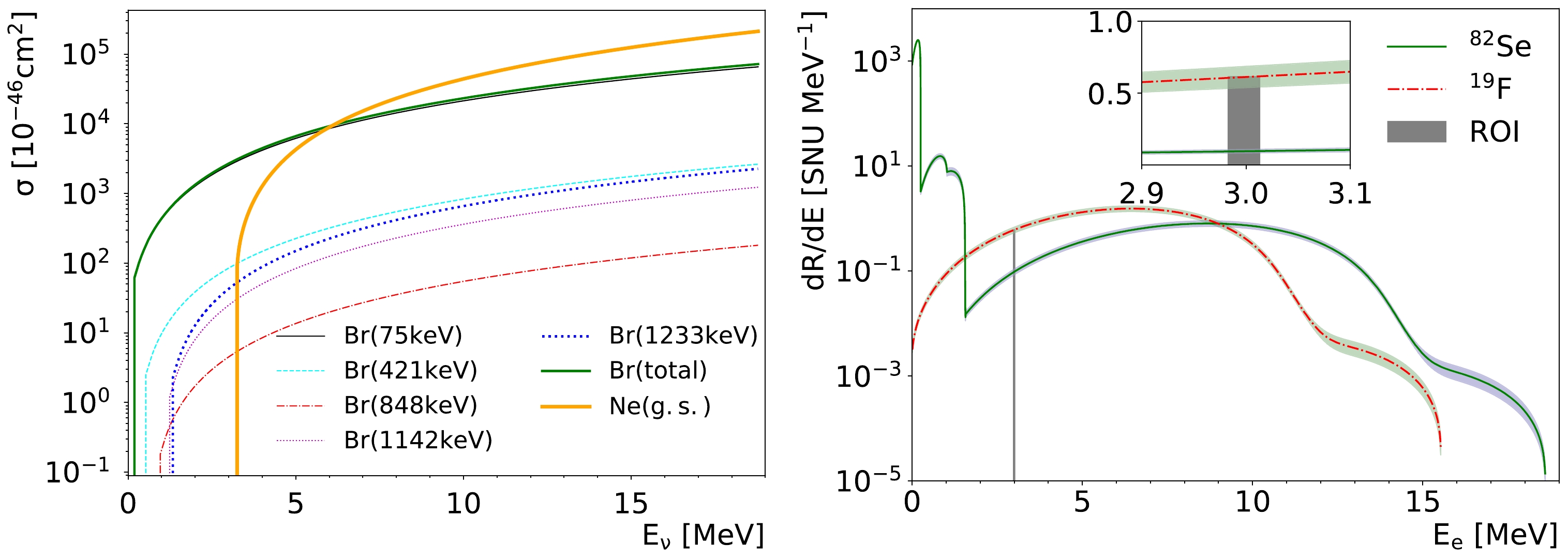
Figure 9. (color online) Interaction cross-section for 82Se and 19F as a function of the neutrino energy (left) and capture rates as a function of the electron energy for 82Se and 19F (right). In the capture rate distribution, only the continuum is shown. The discrete contributions from 10Be and pep to the 82Se case that are far below the ROI are not shown. The uncertainty bands are from the neutrino flux data only. The capture rates near the ROI are shown in the inset.
The excited states will decay to the isomer state 82mBr, the excitation energy of which is 46 keV. 82mBr has a half-life of
$ T_{1/2}=6.13 $ min, decaying either to the ground state of 82Se by radiating a 46 keV gamma or to the ground state of 82Kr via a β decay. The ground state, with$ T_{1/2}=35.28 $ h, decays to excited states of 82Kr via a β decay. Therefore, a long enough time interval exists to separate the CC process and the decay of 82Br and 82mBr. During the deexcitation, the following gamma radiation occurs:$ ^{82}{\rm{Br}}^{*} \to ^{82(m)}{\rm{Br}} + \gamma(s). $

(6) Accordingly, the 75 keV state would release a 29 keV gamma and decay to 82mBr. Therefore, in the detector, we would simultaneously observe an electron from the CC process and a 29 keV gamma. As the energy of the gamma is low and the transitions have large Internal Conversion (IC) coefficients, it loses its energy not far from the electron track. When IC happens, the characteristic X-rays might also be reconstructed. Note that the energy of the X-rays for Se and Br are slightly different:
$ E_{K_{\alpha}}=11.2 $ keV for Se and$ E_{K_{\alpha}}=11.9 $ keV for Br. In principle, one might be able to identify the production of 82Br from its characteristic$ E_{K_{\alpha}} $ if the detector resolution is good enough. However, it is extremely challenging as the energies are very close; an energy resolution better than 6% RMS would be needed. As the half-life of 82mBr is just 6.13 min and it has a 97.4% chance to decay to the ground state while releasing a 46 keV gamma, the coincidence of a 46 keV gamma at the same location could be used to identify the process and reject it. The IC coefficient is huge for this M3 transition. Approximately 12.9% of the 46 keV gamma radiation results in two clusters: one from the$ K_{\alpha} $ X-ray and the other one from the IC electrons. The spread of this low energy gamma is at the cm level, as shown in Fig. 5 (left).For 19F, the process is very similar and much simpler. The transition can go the ground state of 19Ne directly, but the threshold is much higher
$ Q_{\beta}=3.24 $ MeV. Therefore, in the final state, there is only a single electron:$ \nu + ^{19}{\rm{F}} \to ^{19}{\rm{Ne}} + e^- . $

(7) 19Ne has a half-life of 17.22 s. Because the diffusion of the ion in 17.22 s spans only approximately a couple of centimeters, the coincidence of a CC electron and the
$ \beta^- $ decay at the same location within tens of seconds could be used to identify this process.The cross-section can be calculated using Eqn. (4) with
$ B(GT)=1.61 $ and$ B(F)=1 $ from [15]. The differential cross section and capture rate are also shown in Fig. 9. The total capture rate is 8.8 (2.9) SNU (solar neutrino unit,$ =1 \times 10^{-36} $ interactions per target atom per second) without (with) the oscillation effect, and it corresponds to an event rate of 5.1 (1.7) events/(ton·yr).For each CC process, 100k events are simulated within the electron energy in the range of 2.5 to 3.5 MeV. Figure 10 shows the example events of the CC process for 82Se and 19F. Observe from Fig. 5 that the spread and cluster multiplicity are consistent with the single electron events. Note that, in the Br CC process, we have only simulated the 75 keV state, which accounts for 97% of the total capture rate as shown in Fig. 9. If 82Br is excited to higher states, high energy gammas will also be produced. For example, the next major contributing state, the 421 keV state, will decay to the 75 keV state and radiate a gamma with an energy 345 keV. The gamma radiation will increase the spread and number of clusters. Because the signatures of the decays of 82Br and 19Ne are quite different, they are discussed separately in the next two subsections.

Figure 10. (color online) Event display for 82Se CC (left) and 19F CC (right) processes. There are two clusters built in the 82Se CC event. The small cluster containing only two pixels in the bottom right corner, with the blue edge, is from the 11 keV
$ K_\alpha $ X-ray of 82Br. The two small clusters in the 19F event are due to the bremsstrahlung gamma. -
In the beta decays of 82Br and 82mBr,
$ ^{82}{\rm{Br}} \to {}^{82}{\rm{Kr}}^{*} + e^- + \bar{\nu}_e $

(8) $ ^{82m}{\rm{Br}} \to {^{82}{\rm{Kr}}^{(*)}} + e^- + \bar{\nu}_e $

(9) $ ^{82}{\rm{Kr}}^{*} \to {}^{82}{\rm{Kr}} + \gamma(s) $

(10) an electron will be produced, accompanied with gammas if they decay to the excited states of 82Kr. 82Br (g.s.) has ~96.9% chance to decay to the 2.648 MeV excited state of 82Kr. As shown in Fig. 6, multiple photoelectron peaks and the Compton edges from the 82Br decay process can be clearly observed in the reconstructed clusters. As part of the energy will be taken by the neutrino, the majority of the events have a total energy deposition in the detector less than the maximum
$ Q=3.093 $ MeV. Moreover, 82mBr dominantly (~ 88.1%) decays to the ground state of 82Kr, with a small fraction to other excited states: 9.2% to the 777 keV state, 2.1% to the 1475 keV state, and <0.3% to others. Among them, only the Compton edge for the 777 keV state is visible. The Q value for 82mBr is also slightly higher at$ Q=3.14 $ MeV. The spectra of the total energy for both decays are shown in Fig. 11, calculated using BetaShape [49]. Approximately 1.9% of the 82Br(g.s.) decay has a total energy within the 30 keV window around$Q_{\beta \beta}$ . For 82mBr, only 0.0015% is in the ROI window (the 2.4% branching fraction for direct$ \beta^- $ decay is included). The 82Br decay will be a multi-site event due to the multiple gammas; thus, this feature could be used for background rejection. 82mBr decays to the 777 keV state in a similar manner; however, for 82mBr decay to 82Kr (g.s.), there is only a single electron, and one needs to leverage the Bragg peaks to distinguish it.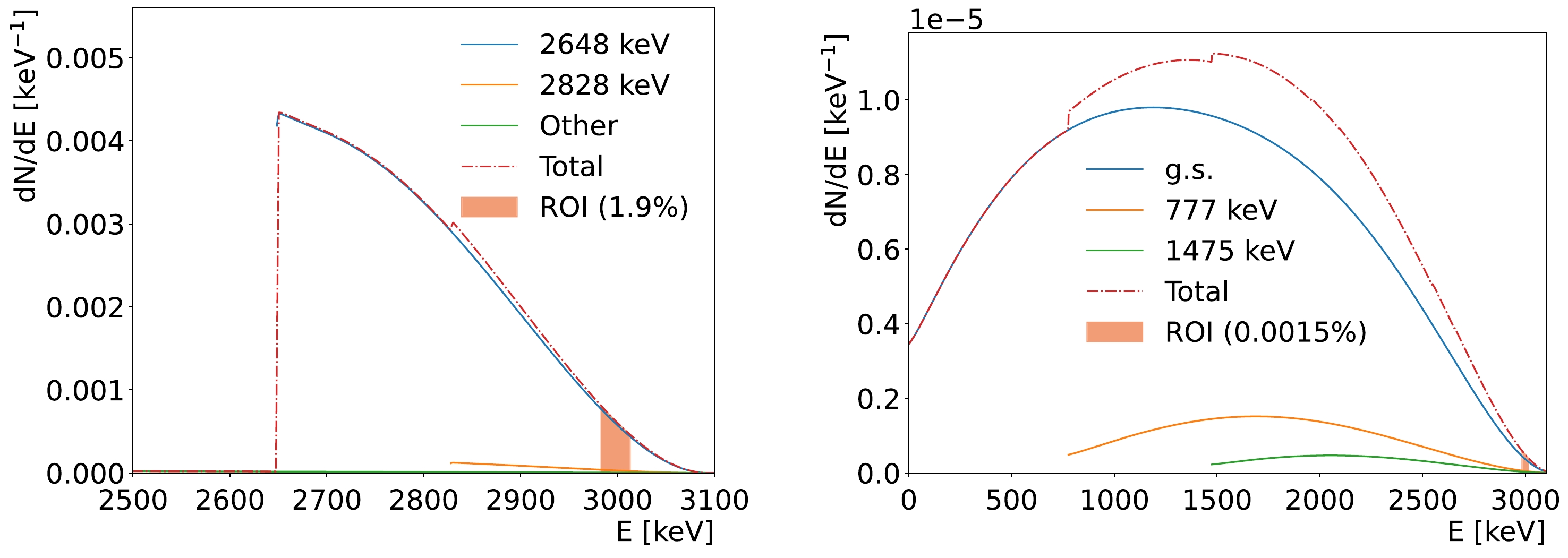
Figure 11. (color online) Distribution of the detectable energy in 82Br (g.s.) decay (left) and 82mBr decay (right). The red dash curves show the total energy, while the breakdown of the main processes to various excited states of 82Kr are shown by solid curves. Filled areas show the ROI with the 30 keV mass window centered at
$ Q_{\beta \beta} $ . The left figure is normalized to unit, and the right one is normalized to the branching fraction of 82mBr beta decay, 2.4%.Considering that 82Br predominately decays to the 2.648 MeV state of 82Kr and the electron from the beta decay usually forms only one cluster, we can calculate the "N-1" cluster energy for cluster i as follows:
$E_{N-1, i}=E_{\rm tot} - E_i$ , where$E_{\rm tot}=\sum_j^N E_j$ is the total energy of the event. When the cluster formed by the electron is removed,$ E_{N-1}=2.648 $ MeV is the excitation energy of 82Kr; for other clusters, it would be random. Therefore, all these events would have at least one cluster having$ E_{N-1} $ close to 2.648 MeV. Fig. 12 shows the distribution of$ E_{N-1} $ for all clusters. The peak at 2.648 MeV can be clearly seen on top of the continuum from random removal. For the 82mBr decay, the 777 keV and 1475 keV peaks are also clearly visible.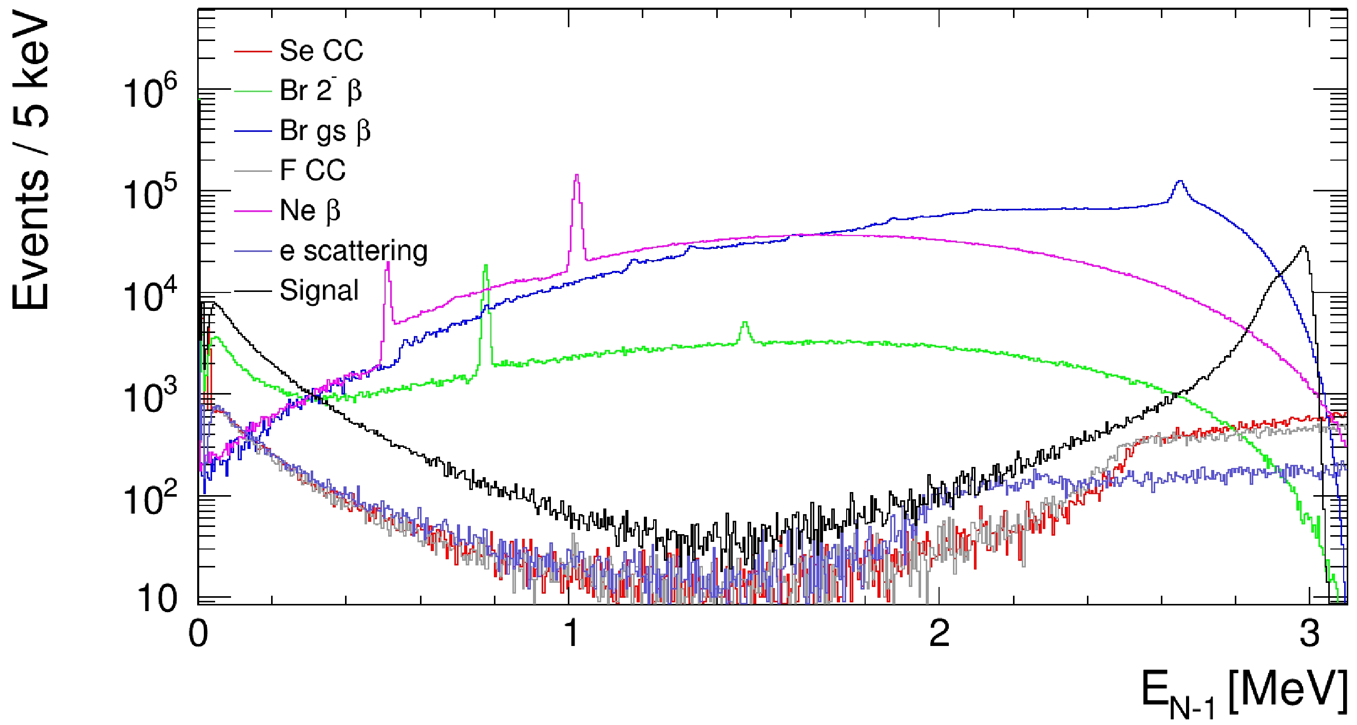
Figure 12. (color online) Distribution of
$ E_{N-1} $ in various processes.One needs to be careful here since, in some 0νββ models, 82Se could decay to the excited states of 82Kr, namely the 777 keV
$ 2^+ $ state and 1488 keV$ 0^+ $ state. In that case, the 777 keV gammaand a 711 keV gamma could also appear in the final state of 0νββ signal events. The 2νββ decay to these states are not experimentally observed yet [50]. -
19Ne has a short half-life of 17.22 s; thus, it will decay back to 19F soon after it is produced through a
$ \beta^+ $ decay:$ ^{19}{\rm{Ne}} \to {^{19}{\rm{F}}} + e^+ + \nu. $

(11) The maximal detectable energy is
$ Q=3.24 $ MeV. The spectra of the total detectable energy are shown in Fig. 13(left). Approximately 0.25% of the events are in the 30 keV wide ROI.
Figure 13. (color online) Distribution of the detectable energy in 19Ne decay (left) and the display of one typical event (right). The contributions from the 110 keV state and 1554 keV state are approximately four orders of magnitude smaller than that of the ground state; thus, they are multiplied by a factor of 1000 to make them visible.
In the detector, the energy deposition comes from a positron track starting at the decay point and two gammas from the electron-positron annihilation at the end point of the positron track. As shown in Fig. 6, the Compton electrons and photoelectrons are reconstructed as clusters. Figure 13 (right) shows a typical event. The energetic gamma could yield multiple Compton scatterings in the detector, resulting in a wide spread of energy and multiple clusters. The number of clusters could be used to reject these background events. By imposing
$ N_{\rm{cluster}}<5 $ , approximately 99.6% of the events are removed. To identify the events, we can use$ E_{N-1} $ to reconstruct the annihilation peak. Observe from Fig. 12 that the peak occurs at approximately 1.022 MeV. Another prominent peak shows up at$ E=0.511 $ MeV, corresponding to the events in which one gamma has escaped the detector. These features could also be used to veto the 19F CC process using the time coincidence as already mentioned in Section III.B. -
If
$ E_\nu $ is higher than the threshold for particle emission ($ S_n=7.593 $ MeV and$ S_p=8.399 $ MeV), 82Br could reach the broad Gamow-Teller resonance (excitation energy$ E_x\approx 12.1 $ MeV and width of$ \approx 5 $ MeV) or IAS (excitation energy 9.576 MeV), decay via emitting a proton (neutron),and transit to 81Se (81Br): $ ^{82}{\rm{Br}}^* \to {^{81}{\rm{Br}}} + n $

(12) $ ^{82}{\rm{Br}}^* \to {^{81}{\rm{Se}}} + p . $

(13) 81Se decays to 81Br through a β decay, with
$ Q_\beta=1588 $ keV:$ ^{81}{\rm{Se}} \to {^{81}{\rm{Br}}} + e^- + \bar{\nu}_e . $

(14) The long lifetime of
$ T_{1/2}=18.45 $ min makes it less signal-like, facilitating the separation of production and decay. Using Eqn. (4) and setting$ B(F)=13.8 $ [14], the event rate for IAS production is calculated to be 0.093 events/(ton·yr).For neutron emission, the signature differs significantly with signal. Therefore, here, we only discuss the proton emission briefly. The energy of the proton from IAS decay is 1.18 MeV. This energy is significantly below our signal ROI, and because the proton is much heavier than the electron, the proton track is much shorter than the electron tracks, as shown in Fig. 5. Considering the low production rate, we conclude that this background could be safely ignored.
-
For Fluorine, 19F is predominant; thus, the contribution from other isotopes is negligible. If 82Se is not enriched to 100%, we also need to consider the CC interaction and subsequent decays of other isotopes. The isotopes with known abundance are listed in Table 1, and their mass differences with the nearby isotopes are shown in Fig. 14.
Isotope Abundance(%) $Q_\beta/{\rm{MeV} }$ 

$Q_{\beta\beta}/{\rm{MeV} }$ 

Br lifetime Br decay 74Se 0.86 6.925 1.209 25.4 min $ \beta^+ $ 

76Se 9.23 4.963 − 16.2 h $ \beta^+ $ 

77Se 7.6 1.365 − 57 h $ \beta^+ $ 

78Se 23.7 3.574 − 6.45 min $ \beta^- $ ,

$ \beta^+ $ 

80Se 49.8 1.870 0.134 17 min $ \beta^- $ ,

$ \beta^+ $ 

82Se 8.82 0.095 2.998 35 h $ \beta^- $ 

Table 1. Information of the Se isotopes and corresponding Br isotopes.
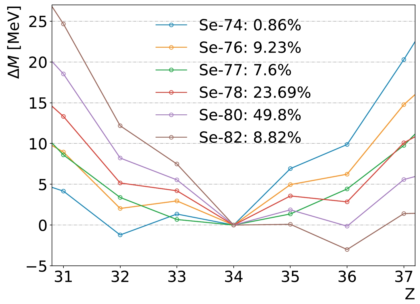
Figure 14. (color online) The mass difference
$ \Delta M=m_{\rm{X}}-m_{\rm{Se}} $ for isotope X with the same A. Only the Se isotopes that have known non-zero abundance values and isotopes that have the same A are shown. The numbers in the legend give the exact abundance of each Se isotope.For the CC process, these isotopes all have higher thresholds and thus smaller capture rates. Moreover, we have shown that, even for the 82Se CC process, the direct background from CC is small because only a small fraction of the outgoing electrons have their energy in the small ROI window. 74Br, 76Br, and 77Br go through a
$ \beta^+ $ decay back to Se. The annihilation peak discussed in Sect. III.D could be used for identification. For 78Br and 80Br, in addition to the$ \beta^+ $ decay to Se, they could go to Kr via$ \beta^- $ decays; however, the released energy is quite small. They may also proceed with an Electron Capture (EC) process, in which case, the visible energy deposit from the X-rays is even smaller. The Br isotopes all have a relatively long lifetime (Table 1). Therefore, the production and decay could be well separated in the detection. -
The background could be divided into two categories: 1) single-electron background, i.e., a background that has a single electron in the final state, with or without a low energy gamma, and 2) multi-site background, i.e., a background that has one or more energetic gammas in the final state. The immediate results of the CC process belongs to the first category. Although, in the 82Br CC process, a 29 keV gamma is observed, its energy is too low to be well separated from the electron track. The β decay of 82mBr is also in this category. The decays of 82Br(g.s) and 19Ne belong to the second category.
For the single-electron background, the main feature that can be used to separate the signal and background is the two Bragg peaks in signal events in contrast to the single Bragg peak in background events. The two Bragg peaks can be clearly seen in the example signal events shown in Fig. 3. There are numerous studies regarding this type of background, and a background suppression factor of 10 or more could be achieved while keeping a high signal efficiency [7, 8, 10, 42]. Therefore, here, we focus on the multi-site background. As there are gammas in these final states, they usually form multiple clusters, and the detection of individual gammas becomes possible. As shown in Fig. 6, the photoelectron peaks and Compton edges can be clearly seen. The peaks are useful to tag the process. For 19Ne decay, we could also see the gamma from annihilation and its Compton edge. In these events, the electron or positron from the
$ \beta^\pm $ decay usually forms a cluster, which often corresponds to the cluster with the highest energy. Figure 15 shows the energy of the leading cluster. As expected, in the signal events, the leading cluster has an energy level close to$ Q_{\beta \beta} $ . However, for 82Br decay, the highest energy cluster is from the 1475 keV gamma. When 82Br decays to the 777 keV excited state, the energy of the electron form this decay could be up to 2.31 MeV; however, the corresponding branching fraction is very small (0.7%). For 19Ne decay, the energy of the positron stops at approximately$ 3.24-1.022=2.2 $ MeV. Thus, a simple cut requiring the energy of the leading cluster to be$ E_0>2.2 $ MeV could remove these events. In the simulation samples containing 1M events, the 82Br decay has 0 events left, while the 19Ne decay has 19 events. An upper limit of the 82Br decay background event rate of$ <0.0001 $ events/(ton·yr) could be set at a 95% C.L. By further requiring$ N_{\rm{clus}}<5 $ , the number of 19Ne decay events is reduced to 2, corresponding to an event rate of$ 0.000003(3) $ events/(ton·yr). The signal efficiency is 98% after the$ E_0>2.2 $ MeV cut and 93% after the$ N_{\rm{clus}}<5 $ cut.
Figure 15. (color online) Distribution of the energy of the leading cluster. The distribution of signal events is scaled by 0.01 to fit the range of other processes.
So far, we have assumed a rather large detector, where almost all the energy of the electrons, positrons, and gammas are collected. In this way, we avoid entangling the physical interactions inside the detector and the boundary effects. In a real detector, there are various boundary effects. For example, the interactions that happen close to the boundaries will result in only part of the energy being deposited inside the fiducial region. The fraction of such events depends on the size and geometry of the detector. When considering the boundary effects, the rejection power of the cut
$ N_{\rm{clus}}<5 $ might degrade because the multi-site background events will have a smaller number of clusters built inside the detector. However, this degradation will be compensated by the reduction of the event rate in the ROI. Figure 16 shows the effect of the detector size on the distribution of the detectable energy and event rate in the ROI. For small detectors, the distribution of the detectable energy shifts to the lower side, with a smaller number of events in the ROI. Notice that the fraction of events in the ROI decreases rapidly as the detector size becomes less than a few meters. This trend is consistent with the energy spread distributions depicted in Fig. 5 (left). Contrarily, the detector size should not affect the$ E_0 $ cut, which remains effective until the detector size becomes smaller than the size of signal events. For a real detector, one would need to optimize the selection cuts based on its size and geometry. The results we obtain here suggest that, using the abovementioned features, one could suppress the multi-site backgrounds with some simple cuts while maintaining a high efficiency for the signal.
Figure 16. (color online) Distributions of the detectable energy within radius
$ R=1 $ m, 5 m, and 20 m from the interaction point (left) and the fraction of events in the ROI as function of R (right) for multi-site background processes.Table 2 presents a summary of the backgrounds. We can effectively reduce the background using the tracking information while maintaining a high efficiency for signal events. Assuming a reduction factor of 10 for the single-electron background, the total background in the 30 keV ROI window should be below 0.001 events/ (ton·yr).
Source All
energyWith
oscillationROI Selection Electron scattering 728.6 481.0 0.00445 $ 0.00395(13)^{*} $ 

82Se CC 63.95 33.88 0.00021 $ 0.000185(4)^{*} $ 

82Br β decay 62.41 33.07 0.63 $<0.0001 $ 

(95% C.L.)82mBr β decay 1.54 0.81 0.00052 $ 0.00037(2)^{*} $ 

19F CC 5.11 1.69 0.0036 $ 0.00318(7)^{*} $ 

19Ne β decay 0.0042 $ 0.000003(3) $ 

Proton emission 0.292 0.093 0 0 Total single-electron
events0.00878 0.00769(15) Total multi-site events 0.63 $<0.0001 $ 

(95% C.L.)Table 2. Summary of the background in unit of events/ (ton·yr). The numbers with * marks in the last column could be further reduced using the energy distribution information in the cluster. The 95% C.L. limits are calculated from the upper limit of the yield 3 events for zero observed events. The last column lists the expected number of events after the selection cuts
$ E_0>2.2 $ MeV and$ N_{\rm{clus}}<5 $ . The uncertainties given in the parentheses are statistical only.The major contributors of the 82Br β decay backgrounds are pp and 7Be neutrinos because of their high fluxes. For ES, 82Se CC, 19F CC, and 19Ne β decay backgrounds, due to the requirement of high
$ E_\nu $ , the contribution from 8B dominates. The high metallicity models predict highter 7Be and 8B neutrino fluxes; thus, more background events are expected. The increases are approximately 3% for 82Br β decay and 20%−30% for other processes. Figure 17 shows a comparison of the total capture rate obtained from various flux data. Note that Fig. 17 (right) for 19F also applies to other backgrounds that require high$ E_\nu $ in the$ ^{8}B $ neutrino range.
Figure 17. (color online) Ratios of the predicted capture rates from various solar neutrino flux data to the baseline (B16-AGSS09 model) for 82Se (left) and 19F (right). The total captures are shown at the bottom, and the relevant breakdowns are shown above them. Horizental bars are obtained by varying the flux by the
$ 1\sigma $ uncertainty given by the model. The flux data are taken from Table 2.1 of [24] and Table Ⅲ of [14].We have shown that several unique features of the background process are useful for background rejection. The successful identification could also be used for solar neutrino studies. With good energy resolution and tracking capability, using a single cluster, we can already observe various characteristic gamma peaks (Fig. 6). Using
$ E_{N-1} $ , we can also obtain the information of the excited states (Fig. 12). A more sophisticated combination of the clusters might increase the efficiency of the tagging. The directional information of the electron scattering would also be useful. As 19F and 82mBr have a short half-life, the coincidence of the time and location could also be used. The feasibility of using this information in solar neutrino experiments should be further studied.Lastly, current results are obtained with some assumptions that are yet to be confirmed experimentally. First, we have assumed a good energy resolution (1% FWHM) that allows us to use a small ROI window. The identification of background processes using the characteristic gamma peaks also demands excellent energy resolution (Figs. 6 and 12). The energy resolution roughly depends on two factors: the number of pixels used to collect the energy of an event and the electrical noise of the pixels. In this study, we have assumed a total noise of 40
$ e^- $ for each readout channel. Recent development shows that this level of low-noise is achievable [9, 51]; however, a readily usable chip does not exist. The number of pixels hit by one event depends on the pitch size and diffusion. The low diffusion of ion drift is confirmed in various measurements [17, 32], but no measurements of ions in 82SeF6 have been conducted so far. The choice of an 8 mm pitch size in this study is based on the results reported in [9], which should be revisited once we have better knowledge about the diffusion and the electrical noise of the readout chip. Second, the cuts we have used, namely the energy of the leading cluster and the number of clusters, require good tracking capability to separate energy clusters. This also depends on the pitch size and diffusion. Finally, if the TPC operates at a different pressure, the pitch size might need to be adjusted to maintain the same performance level. -
Background from solar neutrino is potentially important for neutrinoless double beta decay experiments. Here, the detector response of a high-pressure 82SeF6 gaseous TPC to solar neutrino events is studied via simulations. We found that the background could be effectively rejected using the cluster information, taking advantage of the good energy and spatial resolution of the TPC. By simply setting the energy of the leading cluster as
$ E_0>2.2 $ MeV and number of clusters as$ E_{\rm{clus}}<5 $ , we can reduce the expected number of background to$ <0.001 $ events/(ton·yr) in a 30 keV ROI window around$ Q_{\beta \beta}=2.998 $ MeV. This is sufficient for a ton-yr level exposure. For a larger exposure, further optimization using the real detector setup could be conducted in a similar manner. Given the rich features of the background, it is anticipated that a large detector, equipped with good energy and spatial resolution, would be capable of effectively harnessing these characteristics to achieve an appropriate level of background control.. These features might also be useful for solar neutrino studies, which should be further explored in the future.
Solar neutrino background in high-pressure gaseous 82SeF6 TPC neutrinoless double beta decay experiments
- Received Date: 2023-10-11
- Available Online: 2024-04-15
Abstract: In this study, the possibility of observing a solar neutrino background in a future neutrinoless double beta decay experiment using a high-pressure gaseous 82SeF6 TPC is investigated. Various contributions are simulated, and possible features that could be used for event classification are discussed; two types of backgrounds are identified. The rate of multi-site background events is approximately 0.63 events/(ton·yr) in a 30 keV ROI window. This background could be effectively reduced to less than 0.0001 events/(ton·yr) (95% C.L.) while maintaining a high signal efficiency of 93% by applying a selection based on the number of clusters and energy of the leading cluster. The rate of the single-electron background events is approximately 0.01 events/(ton·yr) in the ROI. Assuming a reduction factor of 10 for the single-electron background events obtained via the algorithms developed for radioactive background rejection, the total background induced by the solar neutrino would be 0.001 events/(ton·yr), which is sufficiently small for conducting ton-level experiments.


 DownLoad: