


 Abstract
 HTML
HTML Reference
 Related
 PDF
PDF


-
Multi-body decays of unstable particles provide richer experimental information than two-body decays owing to the involvement of various intermediate resonances. This makes multi-body decays extremely important in testing the standard model of particle physics and searching for new resonances. For example, the
$ H^0\to Z\mu^+\mu^- $ decay is used to determine the Higgs spin [1], the$ \varLambda_b^0\to J/\psi p K^- $ decay gives rise to the first observation of pentaquark states [2], and recently, the LHCb collaboration observes various sources of violations of charge-conjugation and parity asymmetries in the final-state phase space of B meson decays into three hadrons [3].Following the isobar model [4–6], the total amplitude of a multi-body decay of a hadron can be written as the coherent sum of several sub-amplitudes, each one with a definite helicity for all participating particles. The square of the total amplitude modulus, summed over the initial and final state helicities, gives the final-state probability density distribution (PDF). Unknown parameters, such as the contribution of a new resonance in the decay, spin-parity
$ J^\eta $ , and strength of a specific amplitude, can be extracted by fitting the PDF to real data. Three-body decays$ P_0\rightarrow P_1P_2P_3 $ that involve two spin-$ 1/2 $ fermions and two (pseudo-)scalars (denoted as h in the following equation) are often studied in heavy flavor physics. They are referred to as${\mathrm{2F2P}}$ decays in the$ \varLambda_b^0\rightarrow D^0p h^- $ [7, 8],$ \Xi_b^-\to pK^-K^- $ [9],$ \varLambda_c^+\rightarrow pK^-\pi^+ $ [10], and$ B\rightarrow p \overline{p}^- h $ decays etc. When fitting to experimental data, the PDF of such decays has symmetries that prevent a unique determination of all free parameters, for which there are multiple equivalent solutions. In this paper, this problem is demonstrated, and a possible strategy to fix multiple solutions is proposed. -
Dedicated approaches based on the fundamental symmetry of Lorentz invariance have been adopted to prepare the amplitudes of a multi-body decay, including the tensor [11] and helicity [12] formalisms. In this analysis, the helicity formalism is followed to deal with
${\mathrm{2F2P}}$ decays, namely the$ P_0\rightarrow P_1P_2P_3 $ decays involving two spin-$ 1/2 $ fermions and two (pseudo-)scalars. According to the isobar model, the three-body decay is viewed as a two-step decay comprising a weak decay followed by a strong decay for the problems considered in this analysis. There are a total of 12 degrees of freedom to describe the final-state kinematics, corresponding to the three four-momenta of particles$ P_1 $ ,$ P_2 $ , and$ P_3 $ . After considering the constraints from the energy-momentum conservation between the initial and final states and the fact that the final-state particles are on the mass-shell, only five kinematic variables are independent. Three of the five remaining variables define the direction of the normal of the decay plane formed in the rest-frame of$ P_0 $ and the simultaneous rotation of final-state particles in the decay plane about the normal. If$ P_0 $ is unpolarized (or specifically spinless), the distribution of these three variables carries no physical information. The other two variables define how the energy of the decaying particle is shared among the final state. They can be expressed by a two-body invariant mass,$ m_{ij}\equiv m(P_i, P_j) $ ,$P_i, P_j\in\{P_0, P_1, P_2\}, ~ i\neq j$ , and the helicity angle of the$ P_iP_j $ system [12]. The$ m_{ij} $ distribution in the amplitude is usually described in a model-dependent manner using the Breit-Wigner function [13] for a resonant contribution and an empirical smooth function for a non-resonant component. The helicity angle distribution is determined by Wigner functions [12], which depend on the spin of the$ P_iP_j $ system and rotation angles.Resonances may contribute to the amplitude in any two-body systems as
$P_0\rightarrow R_{ij}P_k, \;R_{ij}\to P_iP_j$ , such that the three-body decay is factorized into a sum of several chained two-body decays. In total, there are three possible decay chains for a${\mathrm{2F2P}}$ decay,$ P^0\rightarrow R(P_1P_2)P_3 $ ,$ P^0\rightarrow R(P_1P_3)P_2 $ , and$ P^0\rightarrow R(P_2P_3)P_1 $ . Resonance R can be a fermion or a boson depending on the decay chain. In the following, the first and second chains are restricted to R being fermions, and the third one is for R being bosons. Each decay in a chain is associated with a helicity-dependent complex coupling to describe the strength, named as helicity coupling$ H_{\lambda_a, \lambda_b}^P $ for particle P decaying into a and b with helicities$ \lambda_a $ and$ \lambda_b $ , respectively. Strong decay$ R_{ij}\to P_iP_j $ conserves the parity symmetry, which requires couplings with positive helicities, and those with negative helicities are only different by a sign,$ H^R_{\lambda_i, \lambda_j}= \eta_i\eta_j\eta_R(-1)^{J_R-J_i-J_j}H^R_{-\lambda_i, -\lambda_j}\equiv \eta^R_{ij} H^R_{-\lambda_i, -\lambda_j} $ . Here, J and η are the corresponding spin and parity quantum numbers of involved particles [12]. For$ J_0=J_i=1/2 $ ,$ J_j=J_k=0 $ , two allowed strong couplings$ H^R_{+1/2}=\eta^R H^R_{-1/2} $ can be absorbed into the weak helicity coupling of the$ P_0\rightarrow R_{ij}P_k $ decay,$ H^0_{+1/2} $ and$ H^0_{-1/2} $ , except for the$ \eta^R=\pm1 $ sign. Here, the other subscript of the helicity couplings, 0, is dropped. Sign$ \eta^R $ measures the parity of the R resonance. For$ J_i=J_j=1/2 $ ,$ J_0=J_k=0 $ , the four strong couplings are related to each other as$ H^R_{+1/2, +1/2}=\eta^R H^R_{-1/2, -1/2} $ ,$ H^R_{+1/2, -1/2}=\eta^R H^R_{-1/2, +1/2} $ , while the single coupling of the$ P_0\rightarrow R_{ij}P_k $ weak decay can be dropped. In the following,$ H^R_+\equiv H^R_{+1/2, +1/2} $ and$ H^R_-\equiv H^R_{-1/2, +1/2} $ are denoted. For$ J_0=J_k=1/2 $ ,$ J_i=J_j=0 $ , the four weak couplings are$H^0_{0, +1/2}, H^0_{-1, +1/2},\; H^0_{0, -1/2}, H^0_{+1, -1/2}$ , while the single coupling of the$ R_{ij}\to P_iP_j $ strong decay can be dropped. These four couplings can be grouped into two parts, denoted as$ H^0_{\pm}\equiv H^R_{0, \pm1/2} $ and$ H^{'0}_\pm\equiv H^0_{\pm1, \mp1/2} $ .As an example, the modulus squared of the unpolarized
$ \varLambda_b^0\rightarrow D^0p h^- $ decay amplitude, contributed by$ R\to D^0p $ resonances, can be expressed as$ \begin{aligned}[b] {\rm{PDF}}= &\sum\limits_{\lambda_{\varLambda_b}\lambda_p}\left|\sum\limits_R H_{\lambda_{R}, \lambda_h}^{\varLambda_b\to Rh}H^{R\to D^0p}_{\lambda_{D^0}, \lambda_p}d^{J^{\varLambda_b}}_{\lambda_{\varLambda_b}, \lambda_R}(\theta_R)d^{J^R}_{\lambda_R, \lambda_p}(\theta_p)F^R(m_{D^0 p})\right|^2\\ =&\left|\sum\limits_R H^R_+ d_{+1/2, +1/2}^{J^R}\left(\theta_p\right) F^R\left(m_{D^0 p}\right)\right|^2\\&+\left|\sum\limits_R \eta^R H^R_- d_{-1/2, -1/2}^{J^R}\left(\theta_p\right) F^R\left(m_{D^0 p}\right)\right|^2 \\ &+\left|\sum\limits_R \eta^R H^R_+ d_{+1/2, -1/2}^{J^R}\left(\theta_p\right) F^R\left(m_{D^0 p}\right)\right|^2\\&+\left|\sum\limits_R H^R_- d_{-1/2, +1/2}^{J^R}\left(\theta_p\right) F^R\left(m_{D^0 p}\right)\right|^2, \end{aligned} $\\

(1) where
$ F^R(m_{D^0p}) $ (shortened to$ F^R $ ) denotes the model describing the mass distribution (the propagator) of resonance R, and$ d^{J^R}_{\lambda_{\varLambda_b}, \lambda_p}(\theta_p) $ is the Wigner small d-function depending on resonance spin$ J^R $ ,$ \varLambda_b $ helicity$ \lambda_{\varLambda_b} $ , proton helicity$ \lambda_p $ , and helicity angle$ \theta_p $ defined by the proton polar angle in the R rest-frame. For the second equality, helicity coupling$ H^{R\to D^0p}_{\lambda_p} $ is absorbed into$ H_{\lambda_{\varLambda_b}}^{\varLambda_b\to Rh} $ , leaving only the$ \eta^R $ sign. Similarly, for the$ B\rightarrow p \overline{p}h $ decay, considering only$ R\to \overline{p}h $ resonances, the PDF is$ {\rm{PDF}} =\sum\limits_{\lambda_p \lambda_{\overline{p}}} \left| \sum\limits_{R}H^{B\to Rp}_{ \lambda_p} H^{R\to \overline{p}h}_{\lambda_{\overline{p}}} d_{\lambda_p \lambda_{\overline{p}}}^{ J^R}\left(\theta_{\overline{p}}\right) F^R\right|^2, $

(2) which has a form identical to the unpolarized
$ \varLambda_b^0\rightarrow D^0p h^- $ decay, by just replacing$ \lambda_{\overline{p}} $ with$ \lambda_{\varLambda_b} $ . In addition, the unpolarized$ \varLambda_b^0\rightarrow R(D^0 h^-)p $ decay has a PDF similar to that of the$ B\rightarrow R(p \overline{p})h $ decay.Helicity couplings of a PDF are unknown parameters that are to be determined by fitting the PDF to data. It is apparent that the helicity couplings in a PDF have a non-measurable global phase. In addition, the magnitude of one helicity coupling is not measurable owing to the PDF normalization. These ambiguities can be removed by fixing
$H_+=1+0\,{\rm i}$ for the contribution of reference resonance R. Moreover, for decays with all resonances in the same chain, the second equation of Eq. (1) and the property of d-functions imply that, if$ \{H_+^R, H_-^R\} $ is a solution, the simultaneous replacement$ H_+^R\to\eta^R H_-^R, H_-^R\to\eta^RH_+^R $ for all resonances is also a solution. These two solutions can be distinguished by requiring, e.g.,$ |H_-|<|H_+| $ for reference R. Flipping the parity of all resonances gives another solution, which can be resolved using the parities of known particles. In Sec. III, it will be shown that additional multiple solutions exist, and more requirements have to be imposed to obtain a unique solution. -
In Eqs. (1) and (2), resonances are only present in one decay chain, such that the initial-state and final-state helicities for different sub-amplitudes are defined in the same reference frames, and are directly summed over incoherently. For decays that have resonances in multiple decay chains, which is usually the case for multibody heavy-flavor decays, the final-state helicities in different chains are, however, not defined in the same reference frames. Additional rotations are needed to align the final-state helicity states, as has been discussed in Refs. [14–17]. In this manuscript, a new strategy is proposed to determine the alignment angles based on the idea that the eigenstates of a particle spin are uniquely fixed by a coordinate system up to a common phase. Let
$ C^{\rm{ref}} $ denote the coordinate system defining the helicity states in the reference chain and$ C^{\rm{alt}} $ denote that for another chain, which can be achieved from$ C^{\rm{ref}} $ by Euler rotation$ C^{\rm{alt}}= R(\alpha, \beta, \gamma)C^{\rm{ref}} $ . Then, the state defined in$ C^{\rm{alt}} $ ,$ |J, \lambda\rangle^{\rm{alt}} $ , is the linear superimposition of those in$ C^{\rm{ref}} $ , given as$ |J, \lambda\rangle^{\rm{alt}} = \sum\limits_{\lambda'}D_{\lambda'\lambda}^J(\alpha, \beta, \gamma)|J, \lambda'\rangle^{\rm{ref}}, $

(3) where
$ D_{\lambda'\lambda}^J(\alpha, \beta, \gamma) $ is the Wigner big D-function. Specifically, for${\mathrm{2F2P}}$ decays, when there are two decay chains of fermionic resonances, Eq. (1) is then extended to$ \begin{aligned}[b] |{\cal{M}}|^2=\;&\sum\limits_{\lambda_{\varLambda_b}\lambda_p}\left|\{{\cal{A}}_{\lambda_{\varLambda_b}\lambda_p}\;{\rm{ of \; ref.\; chain}}\} + \left(\langle 1/2, \lambda_p|\right)^{\rm{ref}} \left(\sum\limits_{\lambda_p'}|1/2, \lambda_p'\rangle^{\rm{alt}}\{ {\cal{A}}_{\lambda_{\varLambda_b}\lambda_p'}\;{\rm{ of\; alt.\; chain}}\}\right)\right|^2\\ =\;&\sum\limits_{\lambda_{\varLambda_b}\lambda_p}\left|\{{\cal{A}}_{\lambda_{\varLambda_b}\lambda_p}\;{\rm{ of\; ref.\; chain}}\} + \sum\limits_{\lambda_p'}D^{1/2}_{\lambda_p, \lambda_p'}(\alpha, \beta, \gamma)\{{\cal{A}}_{\lambda_{\varLambda_b}\lambda_p'}\;{\rm{ of\; alt.\; chain}}\} \right|^2, \end{aligned} $ 
(4) where the completeness of states
$ \sum\limits_{\lambda_p'}|1/2, \lambda_p'\rangle\langle 1/2, \lambda_p'|=1 $ has been inserted, and Eq. (3) is used to obtain the second equation. The Wigner D-functions align the proton helicities in the alternative decay chain to the reference chain. Two coordinate systems$ C^{\rm{ref}} $ and$ C^{\rm{alt}} $ have to be determined in the same reference frame as stressed in Ref. [2]. The Euler angles describing the rotations from one coordinate system to another one are calculated using the equations in Appendix B.With helicity formalism, the coordinate systems for final-state particles are determined sequentially. Let us first define two arbitrary decay chains: the sequence of decays
$P_0\rightarrow R_{1}P_1, \;R_{1}\to R_2P_2, \cdots,\; R_n\to P_{n1}P_{n2}$ is referred to as the R chain, and the$ R ^{\prime} $ chain refers to chained decays of$P_0\rightarrow R^{\prime}_{1}P^{\prime}_1,\; R^{\prime}_{1}\to R^{\prime}_2P^{\prime}_2, \cdots, \;R^{\prime}_n\to P_{n1}P^{\prime}_{n2}$ . Here,$ P_{n1} $ and$ P_{n2}^{(')} $ are the final-state particles, while other$ P_i $ is the final-state or intermediate particles. The alignment of the$ P_{n1} $ helicity states in the two chains is interesting here and those for other final-state particles can be determined following the same strategy. While the R chain and the$ R ^{\prime} $ chain involve different structures and compositions of intermediate states, the set of final states is identical. Given the coordinate system,$ C^i $ , for particle$ R_i $ in the R chain, the coordinate system for$ R_{i+1} $ ,$ C^{i+1} $ , is obtained as the following [2]:$ \begin{aligned}[b] \hat{z}^R_{i+1} &= I(\vec{p}^{R_{i+1}, C^i}) \quad \hat{y}^R_{i+1} = I(\vec{z}^{C^i}\times \vec{p}^{R_{i+1}, C^i})\\ \hat{x}^R_{i+1} &= \hat{y}^R_{i+1}\times \hat{z}^R_{i+1}, \end{aligned} $

(5) where
$ \vec{p}^{R_{i+1}, C^i} $ is the$ R_{i+1} $ momentum in the rest-frame of$ R_i $ , and$ I(\vec{v}) $ takes the unit vector along$ \vec{v} $ . It is clear that within our convention, the coordinate systems for particles$ R_i $ and$ P_i $ are anti-parallel in the z and y directions and parallel in the x direction. For this convention, particles$ R_i $ and$ P_i $ are placed symmetrically in the amplitude, and the parity symmetry relation for the helicity couplings is preserved. An initial coordinate system for$ P_0 $ is given, that for any particle i in the R ($ R^{\prime} $ ) chain,$ C^{i(R)} $ ($ C^{i(R^{\prime})} $ ), can be uniquely defined by repeating Eq. (5). It is apparent that a particle's coordinate system is chain dependent.Systems
$ C^{i(R^{\prime})} $ and$ C^{i(R)} $ are defined in two different reference frames because they are reached from the$ P_0 $ rest-frame by different boost paths. They must be brought to the same reference frame before helicity alignment angles can be calculated from the two systems. The list of sequential boosts that bring the$ P_0 $ rest-frame to the$ P_{f} $ rest-frame in the R chain is defined as$ \{B_1^R, B_2^R\cdots B_{f}^R\} $ and that in the$ R^{\prime} $ chain is defined as$ \{B_1^{R^{\prime}}, B_2^{R^{\prime}}\cdots B_{f}^{R^{\prime}}\} $ , where$ f\equiv n1 $ for a special case in the previous section. For example, for the$ P_0\rightarrow R_{12}P_3, R_{12}\to P_1P_2 $ decay, boost$ B^{R_{12}}_1 $ from the$ P_0 $ rest-frame to the R rest-frame followed by boost$ B^{R_{12}}_2 $ from the$ R_{12} $ rest-frame to the$ P_1 $ rest-frame reaches the$ P_1 $ reference frame in the$ R_{12} $ chain. Now, the three coordinates of$ C^{f(R^{\prime})} $ are extended to four vectors by adding an arbitrary time component (0 for example),$ x^{f(R^{\prime})}\equiv(\hat{x}^{f(R^{\prime})}, 0) $ ,$ y^{f(R^{\prime})}\equiv(\hat{y}^{f(R^{\prime})}, 0) $ , and$z^{f(R^{\prime})}\equiv (\hat{z}^{f(R^{\prime})}, 0)$ . Vector$ x^{f(R^{\prime})} $ can be transformed to the particle$ P_f $ rest-frame through the R chain as$ x^{f(R^{\prime}\to R)} =\left(B_f^R\cdots B_2^RB_1^R\right)\left(B_f^{R^{\prime}}\cdots B_2^{R^{\prime}}B_1^{R^{\prime}}\right)^{-1}x^{f(R^{\prime})}, $

(6) similarly for
$ y^{f(R^{\prime}\to R)} $ and$ z^{f(R^{\prime}\to R)} $ . Here, boost B is represented by Lorentz vectors and is only determined by the momentum of a particle whose rest frame is to be reached. Taking the space components of$x^{f(R^{\prime}\to R)}, y^{f(R^{\prime}\to R)}$ , and$ z^{f(R^{\prime}\to R)} $ , the coordinate system for$ P_f $ in the$ R^{\prime} $ chain transformed to the R chain,$ C^{f(R^{\prime}\to R)} $ , is obtained. The Euler rotations that bring$ C^{f(R)} $ to$ C^{f(R^{\prime}\to R)} $ give the alignment angles needed in Eq. (4), where the R chain is the reference. The same procedure is repeated to determine the helicity alignment angles of all final-state particles.In the case of the
${\mathrm{2F2P}}$ decay, the decay chain can be simplified to$ P_0\rightarrow R_{12}P_3, R_{12}\to P_1P_2 $ . If the decaying particle has$ J=1/2 $ , e.g., the$ \varLambda_b^0 $ baryon in Eq. (1), alignments of its helicities in different chains are also needed. It is appropriately considered by choosing the same initial coordinate system for$ P_0 $ for all decay chains. Similarly, for the$ B\rightarrow p\overline{p}h $ decay in Eq. (2), helicity alignments should be applied for both p and$ \overline{p} $ . Thus, for the${\mathrm{2F2P}}$ decays, two additional Wigner-D rotations are needed for the alternative chain in Eq. (4).Next, our approach is compared with other methods, e.g., that in Ref. [15], for unpolarized
$ \varLambda_b^0\to p K^- \pi^0 $ decays. For these decays, three chains are possible to reach the final state, and alignments of the proton helicity states in different chains are needed. Numeric values show that a β rotation about the y-axis (defined to be the normal of the decay plane in the$ \varLambda_b^0 $ rest-frame) is identical in both methods to align two chains. However, in our method, a rotation by π around the z-axis may be needed since the y-axis of the proton coordinate system may flip the sign in different chains and the β angle is restricted to the$ [0, \pi] $ range. In Fig. 1, the distribution of the β angle that aligns the proton helicity in the$ \varLambda_b^0\to R(p K^-) \pi^0 $ chain (reference) to that in the$ \varLambda_b^0\to R(p \pi^0) K^- $ chain as a function of the two-body invariant-mass squared,$ m^2_{p K^-} $ and$ m^2_{p \pi^0} $ , is shown. At low$ m_{K^-\pi^0} $ , the two proton helicities are almost parallel such that a small β rotation is needed, but they are almost anti-parallel at high$ m_{K^-\pi^0} $ , demanding a large rotation β about the y-axis.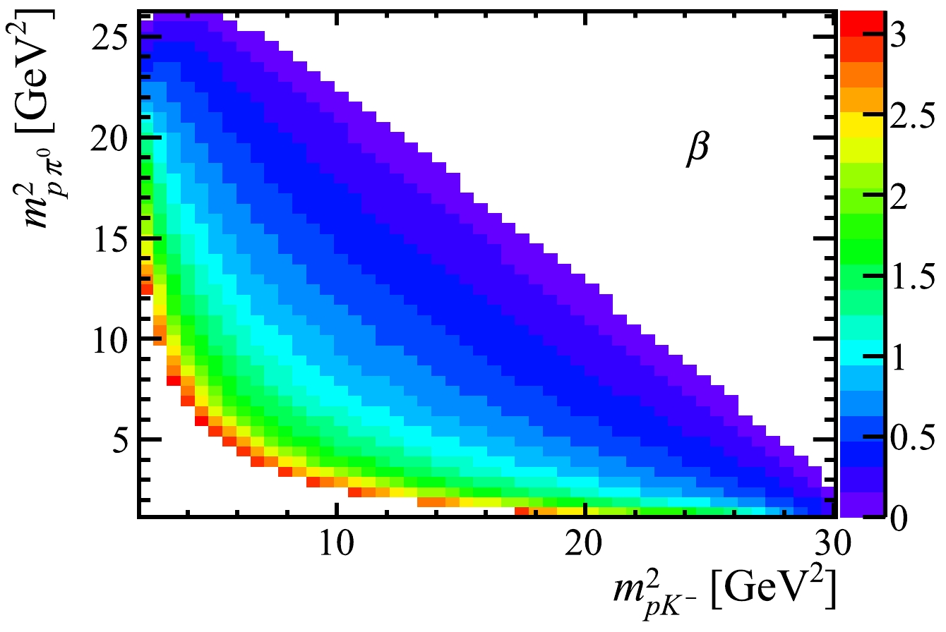
Figure 1. (color online) Distribution of Euler angle
$ \beta\in [0, \pi] $ , which aligns the proton helicity in two decay chains, as a function of the phase-space position. -
In this section, the
$ \varLambda_b^0\to p h^-h^0 $ decay is taken as an example to demonstrate why there are multiple solutions in the amplitude fits of the${\mathrm{2F2P}}$ decays and how to resolve it. As a starting point, only the$ \varLambda_b^0\to R(ph^-)h^0 $ chain is allowed and only two resonances, with$ J^\eta=1/2^- $ , contributing to the amplitude are considered. Secondly, the study is extended to decays with more states and arbitrary$ J^\eta $ . Finally, decays with more than one chain are discussed. -
For only one decay chain with
$ ph^- $ resonances, the PDF of the$ \varLambda_b^0\to p h^-h^0 $ decay can be obtained using Eq. (1) and is shown in Eq. (7)$ \begin{aligned}[b] {\rm{PDF}} =\;&\left|\sum\limits_R H^R_+ d_{+1/2, +1/2}^{1/2}\left(\theta_p\right) F^R\right|^2 \\&+\left|\sum\limits_R H^R_- d_{+1/2, +1/2}^{1/2}\left(\theta_p\right) F^R\right|^2 \\ &+\left|\sum\limits_R H^R_+ d_{-1/2, +1/2}^{1/2}\left(\theta_p\right) F^R\right|^2\\&+\left|\sum\limits_R H^R_- d_{-1/2, +1/2}^{1/2}\left(\theta_p\right) F^R\right|^2, \end{aligned} $

(7) where
$ F^R $ is the model describing the lineshape of the resonances in the$ ph^{-} $ invariant mass spectrum. The relations of Wigner-d functions$ d^j_{m, m'}=d^j_{-m', -m}=(-1)^{m-m^\prime}d_{m', m}^j $ and parity coefficient$ \eta^R=1 $ for the$ J^\eta=1/2^- $ resonances are used to simplify the expression. Notably, since the real d-functions are identical for all resonances, they can be extracted to the outside of the modulus, giving$ \begin{aligned}[b] {\rm{PDF}} =\;&\left(\left|\sum\limits_R H^R_+ F^R\right|^2 +\left|\sum\limits_R H^R_- F^R\right|^2\right)\left[d_{+1/2, +1/2}^{1/2}\left(\theta_p\right)\right]^2 \\&+\left(\left|\sum\limits_R H^R_+ F^R\right|^2+\left|\sum\limits_R H^R_- F^R\right|^2\right)\left[d_{-1/2, +1/2}^{1/2}\left(\theta_p\right)\right]^2\\ =\;&\left(\left|\sum\limits_R H^R_+ F^R\right|^2 +\left|\sum\limits_R H^R_- F^R\right|^2\right)\Big\{\left[d_{+1/2, +1/2}^{1/2}\left(\theta_p\right)\right]^2\\&+ \left[d_{-1/2, +1/2}^{1/2}\left(\theta_p\right)\right]^2 \Big\} \end{aligned} $

$ \begin{aligned}[b]\quad = \left|\sum\limits_R (A^R+{\rm i}B^R) F^R\right|^2 +\left|\sum\limits_R (C^R+{\rm i}D^R) F^R\right|^2, \end{aligned} $

(8) where
$ A^R\equiv{\cal{R}}e({\cal{H}}_+^R) $ ,$ B^R\equiv{\cal{I}}m({\cal{H}}^R_+) $ ,$ C^R\equiv{\cal{R}}e({\cal{H}}^R_-) $ , and$ D^R\equiv{\cal{I}}m({\cal{H}}^R_-) $ represent the respective real and imaginary parts of complex couplings$ H_+ $ and$ H_- $ 1 . For the last equation, the explicit expressions of the Wigner-d functions, which are listed in Table 1, are applied.$ J^R $ 

$ d_{+1 / 2, +1 / 2}^{J^R}\left(\theta\right) $ 

$ d_{-1 / 2, +1 / 2}^{J^R}\left(\theta\right) $ 

$ 1 / 2 $ 

$ \cos \dfrac{\theta}{2} $ 

$ -\sin \dfrac{\theta}{2} $ 

$ 3 / 2 $ 

$ \dfrac{1}{2} \cos \dfrac{\theta}{2}\left(3 \cos \theta-1\right) $ 

$ -\dfrac{1}{2} \sin \dfrac{\theta}{2}\left(3 \cos \theta+1\right) $ 

$ 5 / 2 $ 

$ \dfrac{1}{2} \cos \dfrac{\theta}{2}\left(5 \cos ^2 \theta-2 \cos \theta_p-1\right) $ 

$ -\dfrac{1}{2} \sin \dfrac{\theta}{2}\left(5 \cos ^2 \theta+2 \cos \theta-1\right) $ 

Table 1. Examples of the Wigner-d functions.
The lineshape model,
$ F^R(m_{ph^{-}}) $ , is usually taken to be the form of the Breit-Wigner distribution,$ F^R(m_{ph^-}\mid \mu_R, g_R)=\dfrac{1}{\mu_R^2-m_{ph^-}^2-{\rm i}\mu_R\Gamma_R(m_{ph^-}\mid \mu_R, g_R)}, $

(9) where
$ \mu_R $ and$ g_R $ are the mass and natural width of resonance R, respectively. Then, Eq. (8) is transformed to$ {\rm{PDF}} = \left|\sum\limits_R \frac{(A^R+{\rm i}B^R)}{F^R_{\cal{R}}-{\rm i}F^R_{\cal{I}}} \right|^2+\left|\sum\limits_R \frac{(C^R+{\rm i}D^R )}{F^R_{\cal{R}}-{\rm i}F^R_{\cal{I}}} \right|^2, $

(10) where
$ F^R_{\cal{R}}\equiv \mu_R^2-m_{ph}^2 $ and$ F^R_{\cal{I}}\equiv\mu_R\Gamma_R(m_{ph^{-}}\mid \mu_R, g_R) $ are the real and imaginary parts of the denominator of the Breit-Wigner distribution, respectively. Notably, Eq. (10) holds for any number of$ ph^- $ resonances with$ J^\eta=1/2^{-} $ .For two resonances, by multiplying
$G_1^2\times G_2^2\equiv \left|F^{R_1}_{\cal{R}}-{\rm i}F^{R_1}_{\cal{I}}\right|^2\times \left|F^{R_2}_{\cal{R}}-{\rm i}F^{R_2}_{\cal{I}}\right|^2$ on both sides of Eq. (10), Eq. (10) can be rewritten as$ \begin{aligned}[b] {\rm{PDF}}\times G_1^2 G_2^2=\;&\Big|\left(A^{R_1}+{\rm i}B^{R_1}\right)\left(F^{R_2}_{\cal{R}}-{\rm i}F^{R_2}_{\cal{I}}\right)\\&+\left(A^{R_2}+{\rm i}B^{R_2}\right)\left(F^{R_1}_{\cal{R}}-{\rm i}F^{R_1}_{\cal{I}}\right)\Big|^2\\ &+\Big|\left(C^{R_1}+{\rm i}D^{R_1}\right)\left(F^{R_2}_{\cal{R}}-{\rm i}F^{R_2}_{\cal{I}}\right)\\&+\left(C^{R_2}+{\rm i}D^{R_2}\right)\left(F^{R_1}_{\cal{R}}-{\rm i}F^{R_1}_{\cal{I}}\right)\Big|^2 \\ =&\left[(A^{R_1})^2+(B^{R_1})^2+(C^{R_1})^2+(D^{R_1})^2\right]\\&\times\left[(F^{R_2}_{\cal{R}})^2+(F^{R_2}_{\cal{I}})^2\right]\\ &+\left[(A^{R_2})^2+(B^{R_2})^2+(C^{R_2})^2+(D^{R_2})^2\right]\\&\times\left[(F^{R_1}_{\cal{R}})^2+(F^{R_1}_{\cal{I}})^2\right] \\ &+2\left(A^{R_1} A^{R_2}+B^{R_1} B^{R_2}+C^{R_1} C^{R_2}+D^{R_1} D^{R_2}\right)\\&\times\left(F^{R_1}_{\cal{R}}F^{R_2}_{\cal{R}}+ F^{R_1}_{\cal{I}}F^{R_2}_{\cal{I}}\right) \\ &+2\left(A^{R_1} B^{R_2}-A^{R_2} B^{R_1}+C^{R_1} D^{R_2}-C^{R_2} D^{R_1}\right)\\&\times\left( F^{R_2}_{\cal{R}}F^{R_1}_{\cal{I}}- F^{R_1}_{\cal{R}}F^{R_2}_{\cal{I}}\right), \end{aligned} $

(11) where only helicity coupling parameters
$ \{A^R, B^R, C^R, D^R\} $ are unknown, to be determined from data. Only combinations of these coupling parameters are observed to appear in the PDF. For simplicity, the following notations are made:$ \begin{aligned}[b] P_{1\cdot 1}\equiv&\, (A^{R_1})^2+(B^{R_1})^2+(C^{R_1})^2+(D^{R_1})^2=|H_+^{R_1}|^2+|H_-^{R_1}|^2, \\ P_{2\cdot 2}\equiv&\, (A^{R_2})^2+(B^{R_2})^2+(C^{R_2})^2+(D^{R_2})^2=|H_+^{R_2}|^2+|H_-^{R_2}|^2, \\ P_{1\cdot 2}\equiv&\, A^{R_1}A^{R_2}+B^{R_1}B^{R_2}+C^{R_1}C^{R_2}+D^{R_1}D^{R_2}\\=&{\cal{R}}e(H_+^{R_1*}H_+^{R_2}+H_-^{R_1*}H_-^{R_2}), \\ P_{1\times 2}\equiv&\, A^{R_1}B^{R_2}-A^{R_2}B^{R_1}+C^{R_1}D^{R_2}-C^{R_2}D^{R_1}\\=&{\cal{I}}m(H_+^{R_1*}H_+^{R_2}+H_-^{R_1*}H_-^{R_2}), \end{aligned} $

(12) and when there are more than two resonances,
$ P_{m\cdot n} $ and$ P_{m\times n} $ can be defined similarly for any two resonances$ R_m $ and$ R_n $ . These four P parameters can be determined simultaneously by fitting Eq. (11) to the data. However, as there are eight parameters in the set of$ \{A^R, B^R, C^R, D^R\} $ parameters, four of them are redundant. This is an example of the multiple solution problems that are particularly considered in this manuscript. Notably, when dealing with fit fractions, multiple solutions are physically equivalent. This implies that the fit fraction of each resonance and the interference between any two resonances should be the same for different solutions. However, it should be noted that the helicity couplings differ for different solutions. Therefore, if helicity couplings are required, such as in measurements of CPV using helicity couplings, these solutions are not physically equivalent.The multiple-solution problem for the
${\mathrm{2F2P}}$ decays is rephrased as, given an arbitrary set of$ \{A^R, B^R, C^R, D^R\} $ parameters, there are other sets that will lead to the same P parameters and finally the same PDF value. For two resonances of the same$ J^\eta $ in a single decay chain, according to Eq. (12) not all the free helicity couplings can be determined, four of which must be fixed to reach a stable fit result. For a maximum likelihood fit, the requirement to normalize the PDF removes one additional parameter. This trivial multiple-solution problem is always resolved by fixing$ \left|H_+^R\right|=1 $ for reference resonance R and is not considered anymore in the remaining part of this manuscript. For the special case that only one resonance is present in the decay, only$ P_{1\cdot1} $ remains in Eq. (12), and all four parameters can be fixed after the normalization, the detailed proof is shown in Appendix A. Later on, a strategy to systematically fix redundant helicity couplings to remove multiple solutions will be proposed. -
Equation (11) can be extended to an arbitrary number (N) of resonances with varied
$ J^\eta $ in the same decay chain as$ \begin{aligned}[b]& {\rm{PDF}}\times \prod_{R} G_R^2\\=\;&\left|\sum\limits_R (A^R+{\rm i}B^R) d_{+1 / 2, +1 / 2}^{J^R}\left(\theta\right)\prod_{R^{\prime}, R^{\prime}\neq R} \left(F^{R^{\prime}}_{\cal{R}}-{\rm i}F^{R^{\prime}}_{\cal{I}}\right) \right|^2\\ &+\left|\sum\limits_R \eta^R(A^R+{\rm i}B^R) d_{-1 / 2, +1 / 2}^{J^R}\left(\theta\right)\prod_{R^{\prime}, R^{\prime}\neq R} \left(F^{R^{\prime}}_{\cal{R}}-{\rm i}F^{R^{\prime}}_{\cal{I}}\right) \right|^2\\ &+\left|\sum\limits_R \eta^R(C^R+{\rm i}D^R)d_{+1 / 2, +1 / 2}^{J^R}\left(\theta\right)\prod_{R^{\prime}, R^{\prime}\neq R} \left(F^{R^{\prime}}_{\cal{R}}-{\rm i}F^{R^{\prime}}_{\cal{I}}\right) \right|^2\\ &+\left|\sum\limits_R (C^R+{\rm i}D^R)d_{-1 / 2, +1 / 2}^{J^R}\left(\theta\right)\prod_{R^{\prime}, R^{\prime}\neq R} \left(F^{R^{\prime}}_{\cal{R}}-{\rm i}F^{R^{\prime}}_{\cal{I}}\right) \right|^2. \end{aligned} $

(13) The list of P parameters that appear in the PDF can be defined using those
$ \{A^R, B^R, C^R, D^R\} $ in Eq. (13) as$ \begin{align} P_{m\cdot n}=&\, \eta^{R_m}\eta^{R_n}A^{R_m}A^{R_n}+\eta^{R_m}\eta^{R_n}B^{R_m}B^{R_n}+C^{R_m}C^{R_n}+D^{R_m}D^{R_n}, \\ P_{m\times n}=&\, \eta^{R_m}\eta^{R_n}A^{R_m}B^{R_n}-\eta^{R_m}\eta^{R_n}A^{R_n}B^{R_m}+C^{R_m}D^{R_n}-C^{R_n}D^{R_m}, \end{align} $

(14) where
$ R_m $ and$ R_n $ represent the$ m^{\rm{th}} $ and$ n^{\rm{th}} $ resonances in the list. Oarity coefficients$ \eta^R $ are present in the PDF since they are not identical for all resonances. From Eq. (14), it is clear that the interchange$ A^R \leftrightarrow \eta^R C^R, B^R \leftrightarrow \eta^R D^R $ , for all R will lead to the same P parameters and finally an equivalent PDF. Furthermore, Eq. (14) will have the same form of Eq. (12) by redefining$ \tilde{A}^R\equiv\eta^RA^R $ and$ \tilde{B}^R\equiv\eta^RB^R $ .For N resonances in the same chain, a total of
$ N^2 $ P parameters can be defined from the$ 4N $ degrees of freedom in helicity couplings. For$ N\geq4 $ , the number of P parameters is noticeably not less than the number of independent helicity parameters. However, not all helicity parameters can be uniquely determined from data. To explain the reason, let us define a matrix H of helicity parameters as$ H\equiv \left(\begin{array}{*{20}{l}} {\tilde{A}^{R_1}+{\rm i}\tilde{B}^{R_1} } & {\tilde{A}^{R_2}+{\rm i}\tilde{B}^{R_2} } & {\cdots } & { \tilde{A}^{R_N}+{\rm i}\tilde{B}^{R_N}} \\ {C^{R_1}+{\rm i}D^{R_1} } & { C^{R_2}+{\rm i}D^{R_2} } & {\cdots } & { C^{R_N}+{\rm i}D^{R_N}} \end{array}\right), $

(15) then
$ H^\dagger H $ would give all$ P_{m\cdot n} $ and$ P_{m\times n} $ terms as$(H^\dagger H)_{m, n}=P_{m\cdot n}-{\rm i}P_{m\times n}$ .For any non-trivial
$ 2\times 2 $ unitary matrix$ U\neq I $ ,$ U^\dagger U=I $ , identity$ (U H)^\dagger U H=H^\dagger U^\dagger U H=H^\dagger H $ holds, which means that if the H matrix elements provide a solution for a fit, the elements of$ U H $ provide another solution as$ ((U H)^\dagger U H)_{m, n} $ will lead to the same$P_{m\cdot n}-{\rm i}P_{m\times n}$ . The arbitrariness of U leads to the multiple-solution problem and, in general, any two solutions are linked by a unitary transformation. The$ 2\times 2 $ matrix U belongs to the$ U(2) $ group, which has four independent parameters. The U matrix can be properly chosen to eliminate four free parameters in the H matrix to reach a definite solution.For example, given the solution in Eq. (15), matrix U in the specific form can be calculated as
$ U=\left(\begin{array}{*{20}{c}} {1} & { 0} \\ {0 } & { \exp^{i\psi}} \end{array}\right)\times \frac{1}{{\cal{N}}}\left(\begin{array}{*{20}{c}} {\tilde{A}^{R_1}-{\rm i}\tilde{B}^{R_1} } & { C^{R_1}-{\rm i}D^{R_1}} \\ {-C^{R_1}-{\rm i}D^{R_1}} & {\tilde{A}^{R_1}+{\rm i}\tilde{B}^{R_1}} \end{array}\right), $

(16) where
$ {\cal{N}}=\sqrt{(\tilde{A}^{R_1})^2+(\tilde{B}^{R_1})^2+(C^{R_1})^2+(D^{R_1})^2} $ and ψ is a phase factor to be determined later. It is easily verified that U is unitary. Then,$ H^{''}\equiv U H =\frac{1}{{\cal{N}}}\left(\begin{array}{*{20}{l}} {{\cal{N}}^2} & {(\tilde{A}^{R_1}-{\rm i}\tilde{B}^{R_1})(\tilde{A}^{R_2}+{\rm i}\tilde{B}^{R_2})+(C^{R_1}-{\rm i}D^{R_1})(C^{R_2}+{\rm i}D^{R_2}) } & {\cdots} \\ {0 } & {\exp^{i\psi}\left[(\tilde{A}^{R_1}+{\rm i}\tilde{B}^{R_1})(C^{R_2}+{\rm i}D^{R_2})-(\tilde{A}^{R_2}+{\rm i}\tilde{B}^{R_2})(C^{R_1}+{\rm i}D^{R_1})\right] } & {\cdots} \end{array}\right), $ 
(17) where
$ B^{''R_1}=C^{''R_1}=D^{''R_1}=0 $ have been obtained and ψ can be tuned to set$ D^{''R_2}=0 $ , i.e., four redundant parameters have been fixed. Of course, one can choose another U matrix to get the preferred form of$ H^{''} $ . Therefore, this proves that it is always possible to fix four parameters to zero if resonances are limited to only one chain, reducing the total unknown helicity coupling parameters to$ 4N-4 $ . The detailed form of the transformed H matrix is provided in Appendix C.After fixing four helicity coupling parameters, the number of independent P terms is always no less than the number of remaining free parameters,
$ N^2-(4N-4)= (N-2)^2\geq0 $ . Notably,$ P_{m\times n} $ terms only appear in the PDF if the mass distribution of either the m or n component of the amplitude is complex (e.g., the Breit-Wigner function). If all$ P_{m\times n} $ terms disappear, then the number of P terms reduces to$ N+N(N-1)/2=N(N+1)/2 $ , which is smaller than the number of free coupling parameters$ 4N-4 $ for$ N<6 $ , suggesting additional parameters can be fixed. For example, for two resonances, the following P terms are obtained without$ P_{1\times 2} $ $ \begin{aligned}[b] P_{1\cdot 1}\equiv&\, (\tilde{A}^{R_1})^2, \\ P_{2\cdot 2}\equiv&\, (\tilde{A}^{R_2})^2+(\tilde{B}^{R_2})^2+(C^{R_2})^2, \\ P_{1\cdot 2}\equiv&\, \tilde{A}^{R_1}\tilde{A}^{R_2}, \end{aligned} $

(18) where other four coupling parameters have been set to zero following Eq. (17). Parameter
$ \tilde{A}^{R_1} $ is fixed by$ P_{1\cdot 1} $ ,$ \tilde{A}^{R_2} $ is fixed by$ P_{1\cdot 2} $ , and$ \tilde{A}^{R_1} $ , while$ P_{2\cdot 2} $ can only additionally determine$ (\tilde{B}^{R_2})^2+(C^{R_2})^2 $ . One can fix$ C^{R_2}=0 $ to reach a definite solution. For three resonances in the same chain, one can set$ C^{R_2}=C^{R_3}=0 $ , and so on. This specific decay is not discussed anymore in the following. -
In Sec. III.B, resonances are only considered in the
$ \varLambda_b\to R(ph^-)h^0 $ decay chain (referred to as the reference channel in the following). In this case, the$ H_+ $ ($ H_- $ ) coupling for one resonance only couples to the$ H_+ $ ($ H_- $ ) of other resonances but not the$ H_- $ ($ H_+ $ ) coupling, which can be seen from Eqs. (1) and (2), wherein the same modulus of the helicity for the initial (final) state is the same for different resonances. However, when more than one chain is included in the amplitude, as can be seen from Eq. (4), the$ H_+ $ ($ H_- $ ) couplings of resonances in the reference chain also couple to the$ H_- $ ($ H_+ $ ) couplings of another chain owing to the realignment of the initial- and final-state helicities. One would naively think that all the relative phases fixed as phases of$ H_+ $ and$ H_- $ of the alternative chain are fixed to a$ H_+ $ in the reference chain through one of the moduli. Then, the phases of$ H_+ $ and$ H_- $ in the alternative chain fix the$ H_- $ of the reference chain in other moduli. However, it will be shown that apart from a global phase, which can be used to fix$ {\cal{I}}m(H^{R_1}_+)=0 $ , there is a second degree of freedom to set$ {\cal{I}}m(H^{R_1}_-)=0 $ , where$ R_1 $ is the reference resonance.For a
${\mathrm{2F2P}}$ decay with resonances in two different chains, two kinds of combinations of helicity coupling parameters are present in the PDF. Without the loss of generality, the discussions are based on the first two chains, where intermediate resonances are fermions. In addition to the P terms in Eq. (12) for resonances in the same chain, the following new terms appear between resonances in two different chains$ \begin{aligned}[b] P^S_{m\cdot n}\equiv&\, {\cal{R}}e(H_+^{R_m*}H_+^{R^{\prime}_n}+{\rm{S}}\times H_-^{R_m*}H_-^{R^{\prime}_n}), \\ P^S_{m\times n}\equiv&\, {\cal{I}}m(H_+^{R_m*}H_+^{R^{\prime}_n}+{\rm{S}}\times H_-^{R_m*}H_-^{R^{\prime}_n}), \\ Q^S_{m\cdot n}\equiv&\, {\cal{R}}e(H_+^{R_m*}H_-^{R^{\prime}_n}+{\rm{S}}\times H_-^{R_m*}H_+^{R^{\prime}_n}), \\ Q^S_{m\times n}\equiv&\, {\cal{I}}m(H_+^{R_m*}H_-^{R^{\prime}_n}+ {\rm{S}}\times H_-^{R_m*}H_+^{R^{\prime}_n}), \\ \end{aligned} $

(19) where and R and
$ R^{\prime} $ belong to two different chains,$ {\rm{S}}=+1 $ or$ -1 $ depending on$ R_m, R_n $ parity parameters η and if a π angle is needed to align the initial/final-state helicities in the two decay chains. The detailed derivation of terms in Eq. (19) can be found in Appendix D. As shown, the Q terms represent interferences of the positive and negative helicities of two separate amplitude components.For M resonances in the reference chain and N resonances in the other chain, the total number of independent P and Q terms is
$ M^2+N^2+4MN $ . To generate all these terms, two H matrices similar to that in Eq. (15) are needed, defined as$ \begin{align} H_P\equiv &\left(\begin{array}{*{20}{l}} {H^{R_1}_+ } & { H^{R_2}_+ } & {\cdots } & { H^{R_M}_+ } & { H^{R^{\prime}_{M+1}}_+} & { H^{R^{\prime}_{M+2}}_+ } & {\cdots} & { H^{R^{\prime}_{M+N}}_+} \\ {H^{R_1}_- } & { H^{R_2}_- } & {\cdots } & { H^{R_M}_- } & { H^{R^{\prime}_{M+1}}_-} & { H^{R^{\prime}_{M+2}}_- } & {\cdots} & { H^{R^{\prime}_{M+N}}_-} \end{array}\right), \\ H_Q\equiv &\left(\begin{array}{*{20}{l}} {H^{R_1}_+ } & { H^{R_2}_+ } & {\cdots } & { H^{R_M}_+ } & { H^{R^{\prime}_{M+1}}_-} & { H^{R^{\prime}_{M+2}}_- } & {\cdots} & { H^{R^{\prime}_{M+N}}_-} \\ {H^{R_1}_- } & { H^{R_2}_- } & {\cdots } & { H^{R_M}_- } & { H^{R^{\prime}_{M+1}}_+} & { H^{R^{\prime}_{M+2}}_+ } & {\cdots} & { H^{R^{\prime}_{M+N}}_+ }\end{array}\right), \end{align} $ 
(20) where the
${S}$ coefficient is omitted for simplicity as they will not affect the conclusion. The first M columns of$ H_P $ and$ H_Q $ are identical, and for the$ M+1 $ to$ M+N $ columns, the first and second rows of$ H_Q $ are swapped, which means$ H_- $ s are in the second row of$ H_Q $ . It is verified that$(H_P^\dagger H_P)_{m, n}=P_{m\cdot n}-{\rm i}P_{m\times n}$ and$(H_Q^\dagger H_Q)_{m\leq M, n>M}= Q_{m\cdot n}- $ ${\rm i}Q_{m\times n}$ , giving all the desired P and Q terms.The question is to find unitary matrix U with
$ H_P'\equiv UH_P $ and$ H_Q'\equiv UH_Q $ , such that$ \begin{aligned}[b] (H_P')_{1j}=&(H_Q')_{1j} \\ (H_P')_{2j}=&(H_Q')_{2j} \end{aligned} $

(21) for
$ j\leq M $ (the reference chain), and$ \begin{aligned}[b] (H_P')_{1j}=&(H_Q')_{2j} \\ (H_P')_{2j}=&(H_Q')_{1j} \end{aligned} $

(22) for
$ M<j\leq M+N $ (the alternative chain). Namely, the elements of the transformed$ H_P $ and$ H_Q $ matrices are related. Eq. (21) holds automatically since$ (H_P)_{ij}=(H_Q)_{ij} $ for$ j\leq M $ , corresponding to the reference chain. For the alternative chain, Eq. (22) can be translated to finding a U matrix that meets the requirements$ U \left(\begin{array}{*{20}{l}} {X} \\ {Y} \end{array}\right) = \left(\begin{array}{*{20}{l}} {X'} \\ {Y' }\end{array}\right), \;\; U \left(\begin{array}{*{20}{l}} {Y} \\ {X} \end{array}\right) = \left(\begin{array}{*{20}{l}} {Y'} \\ {X'} \end{array}\right), $

(23) for any
$ X, Y $ , which requires$ \left(\begin{array}{*{20}{l}} {0 } & { 1} \\ {1 } & { 0 }\end{array}\right)U \left(\begin{array}{*{20}{l}} {0 } & { 1} \\ {1 } & { 0} \end{array}\right)=U. $

(24) For a generic unitary matrix of four degrees of freedom,
$ U=\left(\begin{array}{*{20}{l}} {\alpha } & { \beta} \\ {-\beta^*{\rm e}^{{\rm i}\gamma} } & { \alpha^*{\rm e}^{{\rm i}\gamma}} \end{array}\right), $

(25) where α and β are complex and
$ |\alpha|^2+|\beta|^2=1 $ , Eq. (24) implies$ \alpha=\alpha^*{\rm e}^{{\rm i}\gamma},\quad \beta=-\beta^*{\rm e}^{{\rm i}\gamma}, $

(26) which lead to
$ \gamma=2\arg{\alpha} $ and$ \arg{\beta}=\arg{\alpha}\pm \pi/2 $ , and thus eliminate two degrees of freedom. Now, the reduced U matrix has the generic form,$ U(\phi, t)={\rm e}^{{\rm i}\phi}\left(\begin{array}{*{20}{l}} {\cos(t) } & {{\rm i} \sin(t)} \\ { {\rm i} \sin(t) } & {\cos(t)} \end{array}\right), $

(27) with
$ \phi\in(0, 2\pi] $ and$ t\in(-\pi/2, \pi/2] $ . Next, it will be demonstrated that$ (\phi, t) $ parameters can be tuned to set${\cal{I}}m(H_+^{R_1})={\cal{I}}m(H_-^{R_1})=0$ .Multiplying the reduced U matrix in Eq. (27) to
$ H_P $ (only the first column is needed without the loss of generality) reaches$ \begin{aligned}[b] U(\phi, t) H_P= & {\rm e}^{{\rm i}\phi}\left(\begin{array}{*{20}{l}} {\cos(t) } & { {\rm i}\sin(t)} \\ { {\rm i}\sin(t) } & {\cos(t)} \end{array}\right)\times \left(\begin{array}{*{20}{l}} {H_+ } & { \cdots} \\ { H_- } & { \cdots} \end{array}\right)\\ = & {\rm e}^{{\rm i}\phi} \left(\begin{array}{*{20}{l}} {\cos(t) H_+ +{\rm i} \sin(t) H_- } & { \cdots} \\ {\cos(t) H_- +{\rm i} \sin(t) H_+ } & { \cdots} \end{array}\right)\\ \equiv & {\rm e}^{{\rm i}\phi} \left(\begin{array}{*{20}{l}} {H_+' } & { \cdots} \\ {H_-'} & { \cdots} \end{array}\right), \end{aligned} $

(28) where superscript
$ R_1 $ has been omitted. Parameter t is adjusted to make$ H_+ $ and$ H_- $ have a common phase, δ, which can then be removed by choosing$ \phi=-\delta $ . It requires$ \begin{aligned}[b] \tan(\delta)=\;&\frac{ {\cal{I}}m(H_+)\cos(t)+ {\cal{R}}e(H_-)\sin(t)} {{\cal{R}}e(H_+)\cos(t)- {\cal{I}}m(H_-)\sin(t)}\\ =\;&\frac{{\cal{I}}m(H_-)\cos(t)+ {\cal{R}}e(H_+)\sin(t)} {{\cal{R}}e(H_-)\cos(t)- {\cal{I}}m(H_+)\sin(t)},\end{aligned} $

(29) giving
$ \tan(2t)= {\cal{I}}m\left(2H_+H_-^*\right)/\left(|H_+|^2-|H_-|^2\right) $ . Then,$ \delta = \arg(H_+')=\arg(H_-') $ can be determined. It is emphasised that in Eq. (29),$ H_+ $ and$ H_- $ can be chosen to belong to two separate resonances.The discussions above are also valid for the
${\mathrm{2F2P}}$ decays with resonances in all three chains. In this case, four H matrices, built from all possible helicity couplings, would be required to produce all required P and Q terms in the PDF, as$ \begin{aligned}[b]& \left(\begin{array}{*{20}{l}} {H^{R}_+ } & {\cdots } & { H^{R^{\prime}}_+ } & {\cdots} & { H^{R^{\prime \prime}}_+} & {\cdots} \\ {H^{R}_- } & {\cdots } & { H^{R^{\prime}}_- } & {\cdots} & { H^{R^{\prime \prime}}_-} & {\cdots} \end{array}\right), \\& \left(\begin{array}{*{20}{l}} {H^{R}_+ } & {\cdots } & { H^{R^{\prime}}_+ } & {\cdots} & { H^{R^{\prime \prime}}_-} & {\cdots} \\ {H^{R}_- } & {\cdots } & { H^{R^{\prime}}_- } & {\cdots} & { H^{R^{\prime \prime}}_+} & {\cdots} \end{array}\right), \\& \left(\begin{array}{*{20}{l}} {H^{R}_+ } & {\cdots } & { H^{R^{\prime}}_- } & {\cdots} & { H^{R^{\prime \prime}}_+} & {\cdots} \\ {H^{R}_- } & {\cdots } & { H^{R^{\prime}}_+ } & {\cdots} & { H^{R^{\prime \prime}}_-} & {\cdots} \end{array}\right), \\& \left(\begin{array}{*{20}{l}} {H^{R}_+ } & {\cdots } & { H^{R^{\prime}}_- } & {\cdots} & { H^{R^{\prime \prime}}_-} & {\cdots} \\ {H^{R}_- } & {\cdots } & { H^{R^{\prime}}_+ } & {\cdots} & { H^{R^{\prime \prime}}_+} & {\cdots} \end{array}\right), \end{aligned} $

(30) where subamplitude components R,
$ R^{\prime} $ , and$ R^{\prime \prime} $ belong to the three different chains.Now, this proves that, in the generic case, a positive and negative helicity coupling can be set to be real for
${\mathrm{2F2P}}$ decays. Limited to only one decay chain, two more coupling parameters can be fixed to zero. With the matrix transformation method, no more additional freedoms are found to constrain more helicity parameters. Since any two helicity couplings can be fixed to be real, helicity couplings are no longer good physical observables to be compared with theoretical calculations or cross-experiments. Instead, the fit fraction (FF) of the R resonant component, defined as [18]$ {\rm{FF}}_{R}=\dfrac{ \int {\rm{PDF}}(H_+^R, H_-^R, H_+^{R^{\prime}}=H_-^{R^{\prime}}=0\text{ for } R^{\prime}\neq R){\rm d}\Phi}{ \int {\rm{PDF}}(H_+^R, H_-^R, H_+^{R^{\prime}}, H_-^{R^{\prime}}){\rm d}\Phi}, $

(31) only depends on those P and Q parameters, and is thus a quantity independent of conventions on helicity couplings.
-
Pseudo-experiment studies are performed to numerically verify the conclusions reached in the previous section. Events are generated for the
$ B^+\to p \overline{p}^- \pi^+ $ decay composed of a set of resonances, and are then studied with amplitude fits considering the aforementioned strategies to fix helicity couplings. The fit is carried out with the unbinned maximum likelihood method, such that the PDF normalization can be used to fix a helicity coupling parameter in addition to the interesting ones discussed in the previous section. The parameters that maximize the likelihood determine the results of the fit. The Iminuit package [19] is used to maximize the likelihood with respect to free coupling parameters. In the following,$ {\cal{R}}e(H_+^{R_1}) $ is always set to 1 to comply with the PDF normalization requirement. The$ B^+\to \varDelta^{++}(p\pi^+) \overline{p}^- $ decay is taken as the reference channel. -
Here, only the reference channel is considered for the
$ B^+\to p \overline{p}^- \pi^+ $ decay (i.e., only a single decay chain), with three$ \varDelta^{++} $ resonances in the$ \varDelta^{++}\to p\pi^+ $ decay. The masses, widths, and$ J^\eta $ of these$ \varDelta^{++} $ states are listed in the first few rows of Table 2. A random number of about 15000 decays are generated, and the helicity couplings for these resonant contributions are randomly assigned.Resonances $ J^\eta $ 

Mass (MeV/c2) Width /MeV $ \varDelta(1600)^{++} $ 

$ 3/2^+ $ 

1570 50 $ \varDelta(1940)^{++} $ 

$ 3/2^- $ 

2000 400 $ \varDelta(1750)^{++} $ 

$ 1/2^+ $ 

1721 70 $ \varDelta(1700)^{0} $ 

$ 3/2^- $ 

1710 300 $ \varDelta(1900)^{0} $ 

$ 1/2^- $ 

1860 250 Table 2. Resonances considered to generate
$ B^+\to p \overline{p}^- \pi^+ $ decays.Two amplitude fits are performed to the pseudo-data. In the scheme
${\mathrm{A}}$ fit, all helicity couplings are floated apart from$ {\cal{I}}m(H_+^{R_1})=0 $ , while in the scheme${\mathrm{B}}$ fit, four parameters are fixed to zero following the strategy in Sec. III,$ {\cal{I}}m(H_+^{R_1})={\cal{R}}e(H_-^{R_1})={\cal{I}}m(H_-^{R_1})={\cal{I}}m(H_-^{R_2})=0 $ .$ R_1 $ and$ R_2 $ can be arbitrarily chosen among the three resonances. According to our discussions in Sec. III, the two fits should lead to the same likelihood, and there should be no more multiple solutions for the scheme${\mathrm{B}}$ fit.The logarithm likelihood (LL) and the fit fraction of each component obtained with the two fits are listed in Table 3. A detailed table of the fit fraction of each component and the interference between each two components are shown in Appendix E. It is seen that the two fits give identical LL and fit fractions (interferences) up to a numeric precision required by the fitter. Both fit fractions are also consistent with inputs. It confirms that, indeed, four helicity parameters can be fixed to reach the same physical result for a single-chained
${\mathrm{2F2P}}$ decay.Fit LL FF $ \varDelta(1600)^{++} $ 

$ \varDelta(1750)^{++} $ 

$ \varDelta(1940)^{++} $ 

${\mathrm{A}}$ 

$ 29823.04 $ 

0.484655 0.367544 0.148588 ${\mathrm{B}}$ 

$ 29823.04 $ 

0.484653 0.367547 0.148588 Table 3. Logarithm likelihood and fit fraction of each component for two schemes of fitting to a single-chained
${\mathrm{2F2P}}$ decay. In scheme${\mathrm{A}}$ ,$ {\cal{I}}m(H_+^{R_1})=0 $ is fixed, while in scheme${\mathrm{B}}$ ,$ {\cal{R}}e(H_-^{R_1})={\cal{I}}m(H_-^{R_1})={\cal{I}}m(H_-^{R_2})=0 $ are additionally required, where$ R_1=\varDelta(1600)^{++}, R_2=\varDelta(1750)^{++} $ .Notably, the helicity couplings that maximize the likelihood in the scheme
${\mathrm{A}}$ fit depend on the initial values of the free parameters in the fit; they converge to different positions in the parameter space of equivalent solutions. Practically, this makes it difficult to judge whether the fit gives the correct result and to compare different fit results of the same dataset, particularly when the likelihood is complicated by local minima. Additionally, scheme${\mathrm{A}}$ encounters challenges in calculating the error matrix using the usual second partial derivative method as in Iminuit, since the second partial derivative matrix is not invertible. While in general, no such problems exist for the${\mathrm{B}}$ fit. The helicity couplings used to generate pesudo-data and those obtained from the fit using scheme${\mathrm{B}}$ are shown in Table 4, where the uncertainties are reported by the fitter. The fit results are consistent with input values.Coupling Input Fit result $ {\cal{R}}e(H_{\varDelta(1940)}^{+}) $ 

$ \phantom-1.51 $ 

$ \phantom-1.54 \pm 0.06 $ 

$ {\cal{I}}e(H_{\varDelta(1940)}^{+}) $ 

$ \phantom-0.35 $ 

$ \phantom-0.37 \pm 0.11 $ 

$ {\cal{I}}e(H_{\varDelta(1940)}^{-}) $ 

$ -0.78 $ 

$ -0.77 \pm 0.08 $ 

$ {\cal{R}}e(H_{\varDelta(1750)}^{+}) $ 

$ \phantom-0.32 $ 

$ \phantom-0.32 \pm 0.02 $ 

$ {\cal{I}}e(H_{\varDelta(1750)}^{+}) $ 

$ -0.09 $ 

$ -0.10 \pm 0.03 $ 

$ {\cal{R}}e(H_{\varDelta(1750)}^{-}) $ 

$ \phantom-0.52 $ 

$ \phantom-0.50 \pm 0.05 $ 

$ {\cal{I}}e(H_{\varDelta(1750)}^{-}) $ 

$ \phantom-0.40 $ 

$ \phantom-0.41 \pm 0.08 $ 

Table 4. Helicity couplings used to generate pesudo-data and results of the fit using scheme
$\mathrm{B}$ .To further verify our conclusion, the helicity couplings obtained from the scheme
$\verb|A|$ fit with an arbitrary set of initial parameters are transformed using the strategy mentioned in Sec.III.B. The matrix after the transformation is compared with the matrix obtained from the fit in scheme$\verb|B|$ . Matrix$ H_{\verb|A|} $ obtained from the scheme$\verb|A|$ fit and the corresponding unitary transformation matrix U are shown in Eqs. (32) and (33). The transformed matrix of$ H_{\verb|A|} $ ,$H_{\verb|A|_{\rm trans}}$ , and the$ H_{\verb|B|} $ matrix obtained from the scheme$\verb|B|$ fit are shown in Eqs. (34) and (35), respectively. The latter two matrices are identical within the numeric precision of the fitter, as they should be according to the discussion in Sec.III.B.$ H_{\verb|A|}= \left(\begin{array}{*{20}{c}} { 1 } & { -3.5264-5.1065 {\rm i} } & { -3.9552+6.4977 {\rm i}} \\ { 5.0599-8.0252 {\rm i}} & { -0.1755+3.1207 {\rm i}} & { -11.2024+9.9042 {\rm i}} \end{array}\right) $

(32) $ U=\left(\begin{array}{*{20}{c}} {1 } & { 0} \\ { 0 } & { -0.7839-0.6208 {\rm i}} \end{array}\right) \times \left(\begin{array}{*{20}{c}} {1 } & { 5.0599+8.0252 {\rm i}} \\ { -5.0599+8.0252{\rm i} } & { 1} \end{array}\right) $

(33) $ H_{{\verb|A|}_{trans}}=\left(\begin{array}{*{20}{c}} {1-0.3237+0.1019 {\rm i}} & {-1.5396-0.3657 {\rm i}} \\ {0-0.5006-0.4057 {\rm i}} & {0.7669 {\rm i}} \end{array}\right) $

(34) $ H_{\verb|B|}= \left(\begin{array}{*{20}{c}} {1 } & { -0.3236+0.1019 {\rm i} } & { -1.5397-0.3657 {\rm i}} \\ { 0 } & { -0.5007-0.4057 {\rm i}} & { 0.7669 {\rm i}} \end{array}\right) $

(35) -
In this study, two
$ \varDelta^0\to\overline{p}\pi $ resonances, listed in the second half of Table 2, are included in the pseudo-data as a second chain. A total of about 15000 decays are simulated. The$ \varDelta(1600)^{++} $ resonance is taken as the reference resonance ($ i.e. $ ,$ R_1 $ ). To test our fitting strategy obtained in Sec. III, the pseudo-data are fitted with three schemes. In scheme$ {\mathrm{A}}$ ,$ {\cal{I}}m(H_+^{R_1})=0 $ is set, which is expected to have multiple solutions. In scheme$ {\mathrm{B}}$ ,$ {\cal{I}}m(H_+^{R_1})={\cal{I}}m(H_-^{R_1})=0 $ is fixed, which complies with our strategy of fixing multiple solutions. In scheme$ {\mathrm{C}}$ , one additional parameter,$ {\cal{R}}e(H_-^{R_1})=0 $ , is fixed on top of scheme$ {\mathrm{B}}$ , which is expected to have a reduced fit quality owing to insufficient amount of free parameters.The LL and fit fractions for the fits in the three different schemes are listed in Table 5. A detailed table of fit fractions of each component and interferences of each two components are shown in Appendix E. The LL and fit fraction results for
$ {\mathrm{A}}$ and$ {\mathrm{B}}$ are identical within the numeric precision of the fitter. The fit fractions are also consistent with those calculated using input helicity coupling parameters. The error matrix of fit$ {\mathrm{A}}$ cannot be properly calculated by the Iminuit fit package. The fit quality of$ {\mathrm{C}}$ is worse than those of$ {\mathrm{A}}$ and$ {\mathrm{B}}$ , as can be seen from the smaller LL.Fit LL FF $ \varDelta(1600)^{++} $ 

$ \varDelta(1700)^{0} $ 

$ \varDelta(1750)^{++} $ 

$ \varDelta(1900)^{0} $ 

$ \varDelta(1940)^{++} $ 

Sum $ {\mathrm{A}}$ 

24210.79 0.274907 0.051978 0.433754 0.16862 0.060224 0.989483 $ {\mathrm{B}}$ 

24210.79 0.274909 0.051976 0.433758 0.16862 0.060221 0.989484 $ {\mathrm{C}}$ 

24194.10 0.275794 0.054087 0.435634 0.17215 0.055602 0.993271 Table 5. Logarithm likelihood and fit fraction of each resonant component for the three different schemes of fits to two-chained decays. In scheme
$ {\mathrm{A}}$ ,$ {\cal{I}}m(H_+^{R_1}) $ is fixed to zero, and in scheme$ {\mathrm{B}}$ ,$ {\cal{I}}m(H_+^{R_1})={\cal{I}}m(H_-^{R_1})=0 $ are required, while in scheme$ {\mathrm{C}}$ ,$ {\cal{R}}e(H_-^{R_1})=0 $ is additionally required compared to scheme$ {\mathrm{B}}$ , where$ R_1=\varDelta(1600)^{++} $ .In Fig. 2, the one-dimensional invariant mass distributions of pseudo-data are shown, overlaid by the results of fit scheme
$ {\mathrm{A}}$ and$ {\mathrm{B}}$ , showing reasonable consistency between the two fit schemes. Similarly, matrices of helicity couplings obtained from both$ {\mathrm{A}}$ and$ {\mathrm{B}}$ fits, and the transformation matrices are shown in Appendix. 63141592631415927.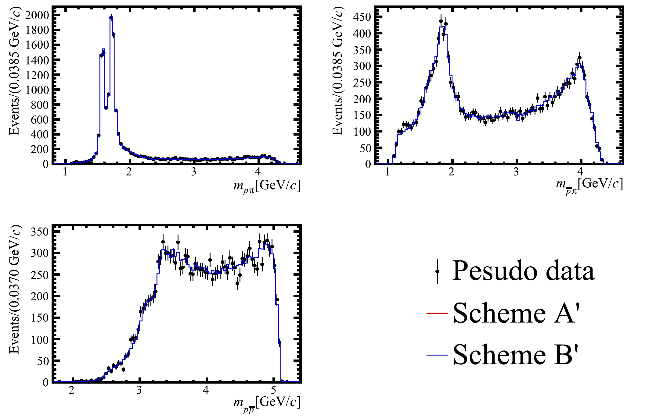
Figure 2. (color online) One-dimensional invariant mass distributions in pseudo-data superimposed by the results in the two fit schemes.
-
Weak decays involving two spin-
$ 1/2 $ fermions and two (pseudo-) scalar particles are very common in heavy flavor physics, and are used for hadron spectroscopy or to study decay properties, with the aim of searching for new hadrons or testing the standard model. In amplitude fits for such decays, the problem of multiple solutions to the helicity couplings is usually encountered, which is studied in detail in this analysis. Detailed studies in this article showed that multiple solutions arise since only combinations of helicity couplings are present in the probability density function rather than each coupling independently. With multiple solutions, the converged position in the parameter space depends on the initial values of the free parameters, making it difficult to judge whether a fit result is the correct answer or not. Moreover, the error matrix of the free parameters cannot be obtained properly using the usual second partial derivative method.A strategy obtained using a matrix transformation method is proposed in our study to resolve the multiple solutions by properly fixing some helicity couplings. In particular, it is found that if all intermediate resonances contribute to a single decay chain, four helicity parameters can be fixed to zero without any loss of fit quality, three of them belonging to a reference resonance and another one for a second resonance. If there are multiple decay chains, it is proved that one can set both the positive and negative helicity couplings of a reference resonance to be real without reducing the fit quality. Using the proposed scheme, there is, in general, no multiple solution problem, and the error matrix of free parameters can be calculated from the second partial derivatives of the likelihood. Pseudo-experiments are generated with one or two decay chains to verify the conclusions of the study. In this analysis, a strategy is also proposed to align the helicity states of initial- and final-state particles defined in two different decay chains, which compares the coordinate systems defining these helicity states. The results of this study will benefit relevant amplitude analyses at LHC, BESIII, and B-factory experiments.
-
If there is only one resonance, Eq. (13) can be simplified to Eq. (36). It is clearly shown that although there are four parameters
$ A^R $ ,$ B^R $ ,$ C^R $ , and$ D^R $ , only the combination of them$\left|A^R+{\rm i}B^R\right|^2+\left|C^R+{\rm i}D^R\right|^2$ can be determined, which is exactly$ P_{1\cdot 1} $ in Eq. (12).$ \begin{aligned}[b]\\[-2pt] {\rm{PDF}}\times G_1^2=\;&\left|(A^R+{\rm i}B^R) d_{+1 / 2, +1 / 2}^{J^R}\left(\theta\right) \right|^2+\left|\eta^R(A^R+{\rm i}B^R) d_{-1 / 2, +1 / 2}^{J^R}\left(\theta\right) \right|^2\\ &+\left|\eta^R(C^R+{\rm i}D^R)d_{+1 / 2, +1 / 2}^{J^R}\left(\theta\right)\right|^2+\left|(C^R+{\rm i}D^R)d_{-1 / 2, +1 / 2}^{J^R}\left(\theta\right) \right|^2\\ =\;&\left|A^R+{\rm i}B^R\right|^2\left(\left| d_{+1 / 2, +1 / 2}^{J^R}\left(\theta\right) \right|^2+\left(\eta^R\right)^2\left| d_{-1 / 2, +1 / 2}^{J^R}\left(\theta\right) \right|^2\right)\\ &+\left|C^R+{\rm i}D^R\right|^2\left(\left(\eta^R\right)^2\left|d_{+1 / 2, +1 / 2}^{J^R}\left(\theta\right)\right|^2+\left|d_{-1 / 2, +1 / 2}^{J^R}\left(\theta\right) \right|^2\right)\\ =\;&\left|A^R+{\rm i}B^R\right|^2\left(\left| d_{+1 / 2, +1 / 2}^{J^R}\left(\theta\right) \right|^2+\left| d_{-1 / 2, +1 / 2}^{J^R}\left(\theta\right) \right|^2\right)\\ &+\left|C^R+{\rm i}D^R\right|^2\left(\left|d_{+1 / 2, +1 / 2}^{J^R}\left(\theta\right)\right|^2+\left|d_{-1 / 2, +1 / 2}^{J^R}\left(\theta\right) \right|^2\right)\\ =\;&\left(\left|A^R+{\rm i}B^R\right|^2+\left|C^R+{\rm i}D^R\right|^2\right)\left(\left| d_{+1 / 2, +1 / 2}^{J^R}\left(\theta\right) \right|^2+\left| d_{-1 / 2, +1 / 2}^{J^R}\left(\theta\right) \right|^2\right) \end{aligned} \tag{A1}$ 
-
Given two coordinate systems,
$ C^0=(\hat{x}^0, \hat{y}^0, \hat{z}^0) $ and$ C^1=(\hat{x}^1, \hat{y}^1, \hat{z}^1) $ , the$ C^1 $ system is reached from the$ C^0 $ system by first rotating α about the$ \hat{z}^0 $ axis, followed by rotating β about the new$ \hat{y}' $ axis, and then rotating γ about the new$ \hat{z}'' $ axis. The three Euler angles are calculated to be$ \alpha = {\mathrm{atan2}} (\hat{z}^1\cdot\hat{y}^0, \hat{z}^1\cdot\hat{x}^0) \tag{B1} $

$\beta = {\mathrm{acos}} (\hat{z}^1\cdot\hat{z}^0) \tag{B2}$

$\gamma = {\mathrm{atan2}} (\hat{z}^0\cdot\hat{y}^1, -\hat{z}^0\cdot\hat{x}^1), \tag{B3} $

with the domains
$ \beta\in[0, \pi] $ ,$ \alpha, \gamma\in(-\pi, \pi] $ . In literature, the$ (\phi, \theta, \psi)\equiv(\alpha, \beta, \gamma) $ notation is also often used. -
As mentioned in Sec. III.B, an H matrix defined as Eq. (15) can be used to determine all the helicity-coupling combinations, and the U matrix defined in Eq. (16) helps to find a definite solution among multiple solutions. In this part, the detailed calculations are shown. Without the loss of generality, only three resonances in the same decay chain are considered for simplicity of writing. Now, Eq. (15) becomes
$ H= \left( \begin{array}{*{20}{l}} {A^{R_1}\eta^{R_1}+{\rm i}B^{R_1}\eta^{R_1} } & { A^{R_2}\eta^{R_2}+{\rm i}B^{R_2}\eta^{R_2}} & { A^{R_3}\eta^{R_3}+{\rm i}B^{R_3}\eta^{R_3}} \\ {C^{R_1}+{\rm i}D^{R_1} } & { C^{R_2}+{\rm i}D^{R_2} } & { C^{R_3}+{\rm i}D^{R_3} } \end{array} \right),\tag{C1} $

where the parity symmetry coefficient η has been explicitly spelled. The U matrix in Eq. (16) is divided into the product of two parts as
$ U=U_1\times U_2 $ , where$ U_1=\left(\begin{array}{*{20}{c}} {p_1-{\rm i}p_2 } & { p_3-{\rm i}p_4} \\ {-p_3-{\rm i}p_4 } & { p_1+{\rm i}p_2} \end{array}\right), \; U_2=\left(\begin{array}{*{20}{c}} {1 } & { 0} \\ {0 } & { \exp^{i\psi}} \end{array}\right), \tag{C2}$

with definitions
$ p_1=A^{R_1}\eta^{R_1}/{\cal{N}} $ ,$ p_2=B^{R_1}\eta^{R_1}/{\cal{N}} $ ,$ p_3= C^{R_1}/{\cal{N}} $ , and$ p_4=D^{R_1}/{\cal{N}} $ , and$ {\cal{N}}=\sqrt{\left(A^{R_1}\right)^2+\left(B^{R_1}\right)^2+\left(C^{R_1}\right)^2+\left(D^{R_1}\right)^2} $ . It is noted that$ p_1^2+p_2^2+p_3^2+p_4^2=1 $ .It is easy to obtain the
$ U_1 $ -transformed H matrix as$ H'\equiv U_1H=\left( \begin{array}{*{20}{c}} {A^{'R_1}} & { A^{'R_2}+ {\rm i}B^{'R_2}} & {A^{'R_3}+{\rm i}B^{'R_3}} \\ {0} & {C^{'R_2}+{\rm i}D^{'R_2}} & {C^{'R_3}+{\rm i}D^{'R_3}} \end{array} \right), \tag{C3}$

with
$ \begin{aligned}[b] A^{'R_1} &=\left(A^{R_1}\right)^2+\left(B^{R_1}\right)^2+\left(C^{R_1}\right)^2+\left(D^{R_1}\right)^2, \\ A^{'R_2} &=A^{R_1}A^{R_2}\eta^{R_1}\eta^{R_2}+B^{R_1}B^{R_2}\eta^{R_1}\eta^{R_2}+C^{R_1}C^{R_2}+D^{R_1}D^{R_2}, \\ B^{'R_2} &=A^{R_1}B^{R_2}\eta^{R_1}\eta^{R_2}-A^{R_2}B^{R_1}\eta^{R_1}\eta^{R_2}+C^{R_1}D^{R_2}-C^{R_2}D^{R_1}, \\ A^{'R_3} &=A^{R_1}A^{R_3}\eta^{R_1}\eta^{R_3}+B^{R_1}B^{R_3}\eta^{R_1}\eta^{R_3}-C^{R_1}C^{R_3}-D^{R_1}D^{R_3}, \\ B^{'R_3} &=A^{R_1}B^{R_3}\eta^{R_1}\eta^{R_3}-A^{R_3}B^{R_1}\eta^{R_1}\eta^{R_3}-C^{R_1}D^{R_3}+C^{R_3}D^{R_1}, \\ C^{'R_2} &=A^{R_1}C^{R_2}\eta^{R_1}-A^{R_2}C^{R_1}\eta^{R_2}-B^{R_1}D^{R_2}\eta^{R_1}+B^{R_2}D^{R_1}\eta^{R_2}, \\ D^{'R_2} &=A^{R_1}D^{R_2}\eta^{R_1}-A^{R_2}D^{R_1}\eta^{R_2}+B^{R_1}C^{R_2}\eta^{R_1}-B^{R_2}C^{R_1}\eta^{R_2}, \\C^{'R_3} &=A^{R_1}C^{R_3}\eta^{R_1}+A^{R_3}C^{R_1}\eta^{R_3}-B^{R_1}D^{R_3}\eta^{R_1}-B^{R_3}D^{R_1}\eta^{R_3}, \\ D^{'R_3} &=A^{R_1}D^{R_3}\eta^{R_1}+A^{R_3}D^{R_1}\eta^{R_3}+B^{R_1}C^{R_3}\eta^{R_1}+B^{R_3}C^{R_1}\eta^{R_3}. \end{aligned}\tag{C4} $

Matrix
$ H' $ multiplied by$ U_2 $ becomes$ H^{''}\equiv U_2H'=\left( \begin{array}{*{20}{c}} {A^{''R_1}} & { A^{''R_2}+ {\rm i}B^{''R_2}} & {A^{''R_3}+ {\rm i}B^{''R_3}} \\ {0} & { C^{''R_2}+ {\rm i}D^{''R_2} } & {C^{''R_3}+{\rm i} D^{''R_3}} \end{array} \right), \tag{C5}$

with
$ \begin{aligned}[b] A^{''R_1} &=A^{'R_1}, \\ A^{''R_2} &=A^{'R_2}, \\ B^{''R_2} &=B^{'R_2}, \\ A^{''R_3} &=A^{'R_3}, \\ B^{''R_3} &=B^{'R_3}, \\ C^{''R_2} &=C^{'R_2} \cos (\psi)-D^{'R_2} \sin (\psi), \\ D^{''R_2} &=C^{'R_2} \sin (\psi)+D^{'R_2} \cos (\psi), \\ C^{''R_3} &=C^{'R_3} \cos (\psi)-D^{'R_3} \sin (\psi), \\ D^{''R_3} &=C^{'R_3} \sin (\psi)+D^{'R_3} \cos (\psi).\\ \end{aligned}\tag{C6} $

Therefore, for
$ \psi=-\arctan(D^{'R_2}/C^{'R_2})+n\pi $ ,$ H^{''} $ becomes$ H^{''}=U_2U_1H=\left( \begin{array}{*{20}{c}} {A^{''R_1}} & { A^{''R_2}+ {\rm i}B^{''R_2}} & {A^{''R_3}+{\rm i}B^{''R_3}} \\ {0} & {C^{''R_2}} & {C^{''R_3}+{\rm i}D^{''R_3}} \end{array} \right). \tag{C7} $

The four free parameters of a
$ 2\times 2 $ $ U(2) $ matrix have been used to eliminate$ {\cal{I}}m(H^{R_1}_+) $ ,$ {\cal{R}}e(H^{R_1}_-) $ ,$ {\cal{I}}m(H^{R_1}_-) $ , and$ {\cal{I}}m(H^{R_2}_-) $ . Of course, they can be alternatively used to remove other helicity-coupling parameters. For example, according to Eq. (45),$ \tan(\psi)=C^{'R_2}/D^{'R_2} $ would remove$ C^{''R_2} $ . In Eq. (15), parity symmetry coefficients$ \eta^{R_m} $ can also be attached to the$ H_-^{R_m} $ couplings (i.e.,$ C^{R_m} $ and$ D^{R_m} $ ) rather than$ H_+^{R_m} $ couplings, which would eventually yield the same result. -
For simplicity of writing, a
${\mathrm{2F2P}}$ decay with a total of two resonances in two channels is considered as an example to demonstrate the study, and the intermediate resonances are taken to be fermions. For decays involving both fermionic and bosonic intermediate resonances, the conclusion is the same. The PDF of this decay has the form,$ \begin{aligned}[b] {\rm{PDF}}=\;& \sum _{m _{b}, m _{p}}\left|H_{m_b}^{R_1} h_{m_p}^{R_1} d_{m_b m_p}^{J^{R_1}} F^{R_1} +\sum _{\lambda_b, \lambda_p} D_{m_b \lambda_b}^{1 / 2} D_{m_p \lambda_p}^{1 / 2} H_{\lambda_b}^{R_2} h_{\lambda_p}^{R_2} d_{\lambda_b \lambda_p}^{J^{R_2}} F^{R_2}\right|^2\\ =\;&\underbrace{\sum _{m _{b}, m _{p}}\left|H_{m_b}^{R_1} h_{m_p}^{R_1} d_{m_b m_p}^{J^{R_1}} F^{R_1}\right|^2}_{T_1} +\underbrace{\sum _{m _{b}, m _{p}}\left|\sum\limits_{\lambda_b, \lambda_p} D_{m_b \lambda_b}^{1 / 2} D_{m_p \lambda_p}^{1 / 2} H_{\lambda_b}^{R_2} h_{\lambda_p}^{R_2} d_{\lambda_b \lambda_p}^{J^{R_2}} F^{R_2}\right|^2}_{T_2} \\ &+\underbrace{2 \sum _{m _{b}, m _{p}}{\cal{R}}e\left[\left(H_{m_b}^{R_1} h_{m_p}^{R_1} d_{m_b m_p}^{J^{R_1}} F^{R_1}\right)^* \sum\limits_{\lambda_b, \lambda_p} D_{m_b \lambda_b}^{1 / 2} D_{m_p \lambda_p}^{1 / 2} H_{\lambda_b}^{R_2} h_{\lambda_p}^{R_2} d_{\lambda_b \lambda_p}^{J^{R_2}} F^{R_2}\right]}_{T_3}, \end{aligned} \tag{D1} $ 
where the two resonances
$ R_1 $ and$ R_2 $ belong to two separate chains, and$ F^{R_1} $ and$ F^{R_2} $ are their respective mass lineshapes. Note that Wigner rotations are needed for both particles b and p in the second chain to align their helicities defined in the second chain to those in the first chain. The H (parity violating) and h (parity conserving) parameters are the corresponding helicity couplings for$ P_0\to R_{ij} P_k $ and$ R_{ij}\to P_i P_j $ decays, respectively.There are three different terms in Eq. (47), labeled as
$ T_1 $ ,$ T_2 $ , and$ T_3 $ , respectively, which will be dealt with separately below. The term$ T_1 $ is simply rewritten as$ \begin{aligned}[b] \left|H_{m_b}^{R_1} h_{m_p}^{R_1} d_{m_b m_p}^{J^{R_1}} F^{R_1}\right|^2 =\;&\left|F^{R_1}\right|^2\left(\left|H_+^{R_1}\right|^2\left[\left(d_{++}^{J^{R_1}}\right)^2+\left(d_{+-}^{J^{R_1}}\right)^2\right]+\left|H_-^{R_1}\right|^2\left[\left(d_{-+}^{J^{R_1}}\right)^2+\left(d_{-}^{J^{R_1}}\right)^2\right]\right)\\ =&\left|F^{R_1}\right|^2\left[\left(d_{++}^{J^{R_1}}\right)^2+\left(d_{+-}^{J^{R_1}}\right)^2\right]\left(\left|H_+^{R_1}\right|^2+\left|H_-^{R_1}\right|^2\right), \\ \end{aligned}\tag{D2} $

where trivial helicity couplings
$ h^{R_1}_{m_p} $ are omitted. This term gives the$ P_{1\cdot1} $ combination of helicity couplings.Term
$ T_2 $ is expanded to$ \begin{aligned}[b] &\sum _{m _{b}, m _{p}}\left|\sum\limits_{\lambda_b, \lambda_p} D_{m_b \lambda_b}^{1 / 2} D_{m_p \lambda_p}^{1 / 2} H_{\lambda_b}^{R_2} h_{\lambda_p}^{R_2} d_{\lambda_b \lambda_p}^{J^{R_2}} F^{R_2}\right|^2\\ =&\left|F^{R_2}\right|^2\left[\sum\limits_{\lambda_b \lambda_p \lambda_b^{\prime} \lambda_p^{\prime}} \sum\limits_{m_b m_p}\left(D_{m_b \lambda_b}^{1/2} D_{m_p \lambda_p}^{1/2} H_{\lambda_b}^{R_2} h_{\lambda_p}^{R_2} d_{\lambda_b \lambda_p}^{J^{R_2}}\right)^*\left(D_{m_b \lambda_b^{\prime}}^{1/2} D_{m_p \lambda_p^{\prime}}^{1/2} H_{\lambda_b^{\prime}}^{R_2} h_{\lambda_p^{\prime}}^{R_2} d_{\lambda_b^{\prime} \lambda_p^{\prime}}^{J^{R_2}}\right)\right] \\ =&\left|F^{R_2}\right|^2\left[\sum\limits_{\lambda_b \lambda_p}\left|H_{\lambda_b}^{R_2} h_{\lambda_p}^{R_2} d_{\lambda_b \lambda_p}^{J^{R_2}}\right|^2\right] =\left|F^{R_2}\right|^2\left[\left(d_{++}^{J^{R_2}}\right)^2+\left(d_{+-}^{J^{R_2}}\right)^2\right]\left(\left|H_+^{R_2}\right|^2+\left|H_-^{R_2}\right|^2\right), \end{aligned}\tag{D3} $

where the unitarity of Wigner-D functions
$ \sum\limits_k D_{m^{\prime} k}^j(\alpha, \beta, \gamma)^* D_{m k}^j(\alpha, \beta, \gamma)=\delta_{m, m^{\prime}} \tag{D4} $

has been used to obtain the third equation. Again, trivial helicity couplings
$ h^{R_2}_{\lambda_p} $ are omitted. This term gives the$ P_{2\cdot2} $ term.Term
$ T_3 $ is expanded as$ \begin{aligned}[b] &2 \sum\limits_{m_b m_p}\left(H_{m_b}^{R_1} h_{m_p}^{R_1} d_{m_b m_p}^{J^{R_1}} F^{R_1}\right)^*\left(\sum\limits_{\lambda_b \lambda_p} D_{m_b \lambda_b}^{1 / 2} D_{m_p \lambda_p}^{1 / 2} H_{\lambda_b}^{R_2} h_{\lambda_p}^{R_2} d_{\lambda_b \lambda_p}^{J^{R_2}}\right) F^{R_2} \\ =&2 F^{R_1 *} F^{R_2} \sum\limits_{m_b m_p \lambda_b \lambda_p}\left(H_{m_b}^{R_1} h_{m_p}^{R_1} d_{m_b m_p}^{J^{R_1}}\right)^*\left(D_{m_b \lambda_b}^{1 / 2} D_{m_p \lambda_p}^{1 / 2} H_{\lambda_b}^{R_2} h_{\lambda_p}^{R_2} d_{\lambda_b \lambda_p}^{J^{R_2}}\right) \\ =&F^{R_1 *} F^{R_2}\sum\limits_{m_b m_p \lambda_b \lambda_p}\left[H_{m_b}^{R_1 *} H_{\lambda_b}^{R_2} h_{m_p}^{R_1} h_{\lambda_p}^{R_2} D_{m_b \lambda_b}^{1 / 2} D_{m_p \lambda_p}^{1 / 2} d_{m_b m_p}^{J^{R_1}} d_{\lambda_b \lambda_p}^{J^{R_2}}\right.\\ & \left.+H_{-m_b}^{R_1 *} H_{-\lambda_b}^2 h_{-m_p}^1 h_{-\lambda_p}^2 D_{-m_b-\lambda_b}^{1 / 2} D_{-m_p-\lambda_p}^{1 / 2} d_{-m_b-m_p}^{J^{R_1}} d_{-\lambda_b-\lambda_p}^{J^{R_2}}\right] \\ =&F^{R_1 *} F^{R_2} \sum\limits_{m_b m_p \lambda_b \lambda_p} {\rm e}^ {-{\rm i} m_b \phi_b-i m_p \phi_p}h_{m_p}^{R_1} h_{\lambda_p}^{R_2}\left[\left(H_{m_b}^{R_1 *} H_{\lambda_b}^{R_2}+{\rm{S}}\times H_{-m_b}^{R_1 *} H_{-\lambda_b}^2\right) d_{m_b \lambda_b}^{1 / 2} d_{m_p \lambda_p}^{1 / 2} d_{m_b m_p}^{J^{R_1}} d_{\lambda_b \lambda_p}^{J^{R_2}}\right], \end{aligned}\tag{D5} $

where the constant
$S \equiv {\rm e}^ {2{\rm i} (m_b \phi_b- m_p \phi_p)}\eta^{R_1} \eta^{R_2}$ is either$ +1 $ or$ -1 $ , depending on Wigner rotation angles$ \phi_b, \phi_p=0 \text{ or }\pi $ and two parity parameters$ \eta^{R_1} \eta^{R_2} $ , but not depending on helicities$ m_b, m_p $ . The second equation is obtained using the fact that for a term with helicities$ \{m_b, m_p, \lambda_b, \lambda_p\} $ , there is always a corresponding one with$\{-m_b, -m_p, -\lambda_b, -\lambda_p\}$ . The parity symmetry for helicity couplings and the relation$ d^j_{-m', -m}=(-1)^{m-m^\prime}d_{m', m}^j $ for d-functions have been used to derive the last (third) equation. Term$ T_3 $ gives the helicity coupling combinations in Eq. (19). -
The fit fraction of each component and the interference between every two components for simulation in Sec. IV.A and Sec. IV.B are shown in this section. Tables A1 and A2 summarize the FFs and interferences for the scheme
${\mathrm{A}}$ and scheme${\mathrm{B}}$ fit data of the single chained$ \varDelta(1600)^{++} $ 

$ \varDelta(1750)^{++} $ 

$ \varDelta(1940)^{++} $ 

$ \varDelta(1600)^{++} $ 

0.484655 $ - $ 0.000420

0.000139 $ \varDelta(1750)^{++} $ 

– 0.367544 $ - $ 0.000507

$ \varDelta(1940)^{++} $ 

– – 0.148588 Table A1. Fit fractions obtained using the scheme
$ {\mathrm{A}}$ fit. The off-diagonal components are for interferences. Owing to the symmetry of the off-diagonal components, only the upper part is displayed while the lower part is replaced with '–'.$ \varDelta(1600)^{++} $ 

$ \varDelta(1750)^{++} $ 

$ \varDelta(1940)^{++} $ 

$ \varDelta(1600)^{++} $ 

0.484653 $ - $ 0.000420

0.000139 $ \varDelta(1750)^{++} $ 

– 0.367547 $ - $ 0.000507

$ \varDelta(1940)^{++} $ 

– – 0.148588 Table A2. Fit fractions obtained using the scheme
$ \mathrm{B} $ fit. The off-diagonal components are for interferences. Owing to the symmetry of the off-diagonal components, only the upper part is displayed while the lower part is replaced with '–'.$ B^+\to p \overline{p}^- \pi^+ $

decay. Tables A3 and A4 summarize the FFs and interferences for the scheme
${\mathrm{A'}}$ and scheme${\mathrm{B'}}$ fit data of the two chained$ B^+\to p \overline{p}^- \pi^+ $ decay. Refer to the text for a detailed description of the fit schemes.$ \varDelta(1600)^{++} $ 

$ \varDelta(1700)^{++} $ 

$ \varDelta(1750)^{++} $ 

$ \varDelta(1900)^{++} $ 

$ \varDelta(1940)^{++} $ 

$ \varDelta(1600)^{++} $ 

0.274907 0.000591 $ - $ 0.000407

$ - $ 0.004418

0.007996 $ \varDelta(1700)^{++} $ 

– 0.051978 0.021664 0.001391 0.001788 $ \varDelta(1750)^{++} $ 

– – 0.433754 0.017107 $ - $ 0.000605

$ \varDelta(1900)^{++} $ 

– – – 0.168620 $ - $ 0.018600

$ \varDelta(1940)^{++} $ 

– – – – 0.060224 Table A3. Fit fractions obtained using the scheme
$ {\mathrm{A}}^{\prime} $ fit. The off-diagonal components are for interferences. Owing to the symmetry of the off-diagonal components, only the upper part is displayed while the lower part is replaced with '–'.$ \varDelta(1600)^{++} $ 

$ \varDelta(1700)^{++} $ 

$ \varDelta(1750)^{++} $ 

$ \varDelta(1900)^{++} $ 

$ \varDelta(1940)^{++} $ 

$ \varDelta(1600)^{++} $ 

0.274909 0.000593 $ - $ 0.000407

$ - $ 0.004418

0.008002 $ \varDelta(1700)^{++} $ 

– 0.051976 0.021663 0.001391 0.001787 $ \varDelta(1750)^{++} $ 

– – 0.433758 0.017109 $ - $ 0.000605

$ \varDelta(1900)^{++} $ 

– – – 0.168620 $ - $ 0.018600

$ \varDelta(1940)^{++} $ 

– – – – 0.060221 Table A4. Fit fractions obtained using the scheme
$ \mathrm{B}^{\prime} $ fit. The off-diagonal components are for interferences. Owing to the symmetry of the off-diagonal components, only the upper part is displayed while the lower part is replaced with '–'. -
The matrices of the helicity couplings obtained from a fit to pseudo-data of two chains of the
$ B^+\to p \overline{p}^- \pi^+ $ decay. Matrix$ H_{\verb|A|^{\prime}} $ is formed by helicity couplings obtained from the scheme$ \verb|A|^{\prime} $ fit with an arbitrary set of initial parameters, which does not converge with the correct error matrix. Matrix$ H_{\verb|B|^{\prime}} $ is built from the helicity couplings obtained from the scheme$ \verb|B|^{\prime} $ fit, which converges properly. Matrix U is a unitary transformation that makes the helicity couplings of the reference resonance real,$ i.e. $ , that of Eq. (27). Under the transformation of U, matrix$ H_{\verb|A|^{\prime}} $ becomes$H_{\verb|A|^{\prime}_{\rm trans}}$ , which is compared to matrix$ H_{\verb|B|^{\prime}} $ .$ H_{{\verb|A|}^{\prime}} = \left(\begin{array}{*{20}{c}} { 1 + 0 {\rm i} } & { -1.9333-2.1460 {\rm i}} & { -3.6880-1.9885 {\rm i}} & { 0.9339 + 2.2177 {\rm i} } & { -2.6738 + 1.4067 {\rm i}} \\ { 2.9673-0.7981 {\rm i}} & { 0.9111 + 0.81522 {\rm i}} & { 0.3518 + 1.3642 {\rm i}} & { -0.0967 - 2.3994 {\rm i}} & { 2.2107 + 1.2875 {\rm i}} \end{array}\right) \tag{F1} $ 
$ H_{{\verb|B|}^{\prime}}=\left(\begin{array}{*{20}{c}} {1+0{\rm i} } & { -1.0658-2.8354 {\rm i} } & { -2.810-3.1818 {\rm i} } & { -0.0919 + 2.4206 {\rm i} } & { -2.8802 + 0.2964 {\rm i}} \\ { 2.9672+0 {\rm i}} & { 0.3124 + 1.2448 {\rm i}} & { -0.4720+1.8034 {\rm i}} & { 0.9904-2.4216 {\rm i}} & { 1.8090+2.3633 {\rm i}} \end{array}\right) \tag{F2} $

$ H_{{\verb|A|}_{trans}^{\prime}}=\left(\begin{array}{*{20}{c}} { 1 + 0 {\rm i} } & { -1.0656-2.830542 {\rm i} } & { -2.8088-3.1761 {\rm i}} & { -0.0914 + 2.4174 {\rm i}} & { -2.8747 + 0.2985 {\rm i}} \\ { 2.9629 + 0 {\rm i}} & { 0.3130 + 1.2441 {\rm i}} & { -0.4699 + 1.8008 {\rm i}} & { 0.9868-2.4189 {\rm i}} & { 1.8088 + 2.3600 {\rm i}} \end{array}\right) \tag{F3} $

$ U = (0.9473 + 0.3203 {\rm i}) \times \left(\begin{array}{*{20}{c}} { 0.1132 + 0 {\rm i}} & { 0.9935 {\rm i}} \\ {0.9935 {\rm i}} & { 0.1132 + 0 {\rm i}} \end{array}\right) \tag{F4} $

A scheme to fix multiple solutions in amplitude analyses
- Received Date: 2023-11-01
- Available Online: 2024-05-15
Abstract: Decays of unstable heavy particles usually involve the coherent sum of several amplitudes, like in a multiple slit experiment. Dedicated amplitude analysis techniques have been widely used to resolve these amplitudes for better understanding of the underlying dynamics. In special cases where two spin-1/2 particles and two (pseudo-) scalar particles are present in the process, multiple equivalent solutions are found owing to intrinsic symmetries in the summed probability density function. In this study, the problem of multiple solutions is discussed, and a scheme to overcome this problem is proposed by fixing some free parameters. Toys are generated to validate the strategy. A new approach to align the helicities of initial- and final-state particles in different decay chains is also introduced.


 DownLoad: