


 Abstract
 HTML
HTML Reference
 Related
 PDF
PDF


-
In recent years, the detection of gravitational waves from binary black hole mergers [1] and the upcoming gravitational wave detection missions such as the LISA [2], Taiji [3], and Tianqin [4] projects have underscored the urgency and significance of modeling the two-body problem in general relativity. Specifically, the motion of a small body in extreme mass ratio inspirals can be treated as a perturbation of timelike geodesic motion, which can be effectively modeled using the self-force approach [5]. Accretion disks around rotating black holes are intimately connected to the innermost stable circular orbit (ISCO) or unstable circular geodesics [6]. The investigation of plunging and deflecting timelike geodesics offers valuable insights into the Penrose process [7] and the two-body scattering problem [8]. Furthermore, the recent interest in analyzing black hole images [9−13] is closely tied to null and timelike Kerr geodesics.
The study of Kerr geodesics began since the Kerr solution was discovered in 1963 [14]. In 1968, Carter found an extra conserved quantity called the Carter constant [15] during the geodesic motion in Kerr spacetime, which was further discussed in [16]. Wilkins [17] studied the bound geodesics in Kerr spacetime. In [18], Bardeen studied the timelike and null geodesics, which were further analyzed in [19−21]. Chandrasekhar [22] reviewed the achievements on Kerr geodesics in the early stage. Twenty years ago, Mino introduced Mino time, decoupling the radial and polar motion [23]. The bound geodesics were revisited, and the explicit form of the geodesics in terms of fundamental orbital frequencies was given in [24]. Later, these geodesics were further analyzed using separatrix and elliptic functions [25−27]. It was proven that only trapped orbits are allowed for negative energy geodesic motion in the ergoregion [28]. In recent years, the geodesic motion in the near-horizon region of high-spin black holes has been analyzed [29−32]. Gralla and Lupsasca provided analytical solutions for null geodesics in Kerr spacetime [33]. The full classification of timelike radial geodesic motion was performed in [34]. A new method for calculating inspirals from the innermost stable circular orbit (ISCO) was introduced in [35]. Analytical solutions for geodesics related to circular and innermost stable spherical orbits in the phase space have been obtained [36, 37]. Nevertheless, compared with the classification of the equatorial geodesics in [34], some classes of orbits, such as trapped orbits associated with parameters governing bound and deflecting motion, still lack explicit analytical solutions.
In this study, we revisit the equatorial timelike geodesic motion in Kerr spacetime. Specifically, we focus on the generic orbits related to the "special" orbits, such as circular, bound, and deflecting orbits, i.e., the geodesic classes in the region
$ \ell^u\leq\ell\leq\ell^s $ of the phase space in Figure 8 of [34]. The motion on the equatorial plane is mainly dominated by the radial motion, which is constrained by the radial potential. For the radial potential on the equatorial plane, there is always a root located at$ r=0 $ . Setting the mass of the black hole and the particle$ M=\mu=1 $ , the radial potential can be reduced to a cubic polynomial of r,$ \begin{array}{*{20}{l}} R(r)=(E^2-1)r^3+2r^2+(a^2(E^2-1)-\ell^2)r+2(\ell-aE)^2, \end{array} $

(1) where E and
$ \ell $ are the conserved energy and angular momentum, and a denotes the spin of the black hole. For the orbits that plunge into the black hole, the angular momentum must satisfy [34]$ \ell\le\ell_+=\dfrac{2Er_+}{a}, $

(2) where
$ \ell_+ $ is the angular momentum of the root structure with one root touching the horizon.Analyzing the roots of the radial potential and its derivatives, one can obtain the classification of the radial motion in the parameter space, as shown in Figure 8 of [34]. For the convenience of the discussion, we introduce the notation of the root structures in Table 1 following [34].
Notation Denotes Notation Denotes $ \vert $ 

outer horizon $ \bullet $ 

simple roots (turning points) $ + $ 

allowed region $ \bullet \bullet $ 

double roots (circular orbits) $ - $ 

disallowed region $ \bullet\bullet\bullet $ 

triple roots (ISCO) $ \rangle $ 

radial infinity $ {\vert \bullet } $ 

roots touching the horizon Table 1. Notations for the root structures on the equatorial plane.
The remainder of this paper is organized as follows. In Section II, we discuss the geodesics related to the circular orbits. In Section III, we present the geodesics associated with the bound and deflecting orbits. The marginal orbits are discussed in Section IV. Finally, we provide a summary of our results in Section V. In Appendix A, we give the definition of elliptic integrals used in this paper. We prove that the solution of trapped orbits associated with bound and deflecting orbits can return to the stable and unstable cases in Appendix B. During the preparation of this paper, Adam, Eva, and Patryk solved the non-equatorial Kerr geodesic motion in terms of Weierstrass elliptic functions [38]. We compare the deflecting orbits with the non-equatorial results in [38] as a consistency check in Appendix C.
-
In this section, we suppose the circular orbit locates at
$ r_* $ . The angular momentum and the energy of the circular orbits are obtained by solving for$ R(r_*)=0 $ and$ R'(r_*)=0 $ ,$ \ell_{a,b}(E,r_*)=\frac{-2aE\mp\sqrt{r_*(2+(E^2-1)r_*)\Delta(r_*)}}{r_*-2}, $

(3) $ E_{\pm}^{(1)}(r_*)=\pm\frac{(r_*-2)\sqrt{r_*}- a}{r_*^{3/4}\sqrt{(r_*-3)\sqrt{r}-2a}}, $

(4) $ E_{\pm}^{(2)}(r_*)=\pm\frac{(r_*-2)\sqrt{r_*}+ a}{r_*^{3/4}\sqrt{(r_*-3)\sqrt{r}+2a}}. $

(5) The branches of the solution are
$ \begin{array}{*{20}{l}} (\ell_a(E_+^{(1)}),E_+^{(1)}), (\ell_a(E_-^{(2)}),E_-^{(2)}), (\ell_b(E_-^{(1)}),E_-^{(1)}), (\ell_b(E_+^{(2)}), E_+^{(2)}); \end{array} $

(6) Based on the analysis in [34], the allowed circular motion are
$ (\ell_a(E_+^{(1)}),E_+^{(1)}) $ and$ (\ell_b(E_+^{(2)}), E_+^{(2)}) $ , which can be reduced to$ \ell^{(1),(2)}(r_*)=\pm\frac{r_*^2\mp2 a \sqrt{r_*}+ a^2}{r_*^{3/4} \sqrt{r_*^{3/2}-3 \sqrt{r_*}\pm2 a}}, $

(7) $ E^{(1),(2)}(r_*)=\frac{(r_*-2)\sqrt{r_*}\pm a}{r_*^{3/4}\sqrt{(r_*-3)\sqrt{r_*}\pm2a}}, $

(8) where branch
$ (1) $ with the upper sign denotes the prograde circular obits, and branch$ (2) $ with the lower sign denotes the retrograde orbits.Here, we introduce the special values in [31]
$ r_c^{(1)}=2-a+2\sqrt{1-a}, $

(9) $ r_c^{(2)}=2+a+2\sqrt{1+a}, $

(10) $ r_*^{(1)}=2+\cos\left(\frac{2\arcsin a}{3}\right)-\sqrt{3}\sin\left(\frac{2\arcsin a}{3}\right), $

(11) $ r_*^{(2)}=2+\cos\left(\frac{2\arcsin a}{3}\right)+\sqrt{3}\sin\left(\frac{2\arcsin a}{3}\right), $

(12) where
$ r_c^{(1),(2)} $ are obtained by solving$ E^{(1),(2)}=1 $ , and$ r_*^{(1),(2)} $ are obtained under the condition that$ E^{(1),(2)} $ are real, such that, at$ r_*^{(1),(2)} $ , we have$ E^{(1),(2)}\to \infty $ .Circular orbits with energy
$ |E|\neq1 $ Ignoring the ISCO, there are three types of root structures related to the circular orbits,$ \vert+\bullet\bullet+\bullet-\rangle $ and$ \vert+\bullet-\bullet\bullet-\rangle $ for$ |E|<1 $ , and$ \vert+\bullet\bullet+\rangle $ for$ E>1 $ . The allowed orbits in the$ + $ region have the same angular momentum and energy as the corresponding circular orbits. Note that no permitted orbits are associated with circular orbits with energy$ E\leq-1 $ . Now consider the radial potential in the following form:$ \frac{R(r)}{E^2-1}=(r-r_1)(r-r_*)^2, $

(13) comparing with (1) and replacing
$ (E,\ell) $ with the angular momentum and energy of the prograde and retrograde circular orbits$(E^{(1),(2)},\,\ell^{(1),(2)})$ , another root can be obtained in terms of the position of the circular orbits$ r_* $ ,$ r_1=r_{1^\pm}=\frac{2 r_* \left(a\mp\sqrt{r_*}\right)^2}{-a^2\pm4 a \sqrt{r_*}+(r_*-4) r_*}, $

(14) where the
$ + $ and$ - $ indices denote the prograde and retrograde orbits.With the energy
$ |E|<1 $ , when$ r_{1^\pm}=r_*=r_{I^\pm} $ , the double root and the single root merge into a triple root, forming the innermost stable circular orbits (ISCO)$ \vert+\bullet\bullet\bullet -\rangle $ with the angular momentum and energy$ (\ell_{I^{\pm}}, E_{I^{\pm}}) $ , which has been revisited in [35]. When$ r_+<r_{1}<r_* $ , the circular orbits are stable with the root structure$ \vert+\bullet-\bullet\bullet-\rangle $ , the orbits in the$ + $ region$ r_+<r<r_{1} $ are trapped orbits$ \mathcal{T}^s $ ; when$ r_{1}>r_* $ , the circular orbits are unstable with the root structure$ \vert+\bullet\bullet+\bullet-\rangle $ , the orbits in the first$ + $ region$ r_+<r<r_* $ are whirling trapped orbits$ \mathcal{W} \mathcal{T}^u $ , and the orbits in the second$ + $ region$ r_*<r<r_{1} $ are whirling bound orbits$ \mathcal{W} \mathcal{B}^u $ or homoclinic orbits$ \mathcal{H}^u $ .With the energy
$ E>1 $ , the other root$ r_1<0 $ , but one can easily prove that we always have$ -r_1>r_* $ for$ r_*>r_+ $ . The circular orbits are unstable with the root structure$ \vert+\bullet\bullet+\rangle $ , the orbits in the first$ + $ region$ r_+<r<r_* $ are whirling trapped orbits$ \mathcal{W} \mathcal{T}^u $ , and the orbits in the second$ + $ region$ r>r_* $ are whirling deflecting orbits$ \mathcal{W} \mathcal{D}^u $ .The r and ϕ components of the 4-velocity of the orbits in the
$ + $ region can be expressed in terms of the parameters of related circular orbits,$ U^r=\frac{ {\rm{d}} r}{ {\rm{d}} \tau}=\pm\frac{\sqrt{(E^2-1)r(r-r_{1})(r-r_*)^2}}{r^2}, $

(15) $ U^{\phi}=\frac{ {\rm{d}}\phi}{ {\rm{d}} \tau}=\frac{2aE+\ell(r-2)}{r\Delta(r)}, $

(16) where
$ \Delta(r)=(r-r_-)(r-r_+) $ , the sign$ + $ denotes the outgoing orbits, and$ - $ denotes the ingoing orbits. Particularly, for the ϕ motion related to the radial motion, we have$ \frac{ {\rm{d}}\phi}{ {\rm{d}} r}=\frac{ {\rm{d}}\phi}{ {\rm{d}}\tau}\frac{ {\rm{d}}\tau}{ {\rm{d}} r}=U^\phi\frac{ {\rm{d}}\tau}{ {\rm{d}} r}. $

(17) From now on, we only discuss the ingoing orbits. For the outgoing orbits, one can simply flip the sign by symmetry.
-
We first discuss the ingoing prograde orbits with the root structure
$ \vert+\bullet\bullet+\bullet-\rangle $ . Then, the energy is confined in the region$ E_{I^\pm}<E^{(1),(2)}<1 $ , and the locations of the unstable circular orbits are confined in the region$ r_c^{(1),(2)}<r_*<r_{I^\pm} $ .The whirling trapped orbits (
$ \mathcal{W} \mathcal{T}^u $ ) related to the unstable circular orbits, which represent the allowed motion in the first$ + $ region$ r_+<r<r_*<r_{1} $ , asymptotically approach the unstable circular orbits. For$ \mathcal{W} \mathcal{T}^u $ and the orbits inside the horizon$ 0<r<r_+ $ , the ingoing radial velocity is given by$ U^r=\frac{ {\rm{d}} r}{ {\rm{d}}\tau}=-\frac{(r_*-r)\sqrt{(E^2-1)r(r-r_{1})}}{r^2}, $

(18) which can be reorganized as
$ -\sqrt{1-E^2} {\rm{d}}\tau=\frac{1}{\left(\dfrac{r_*}{r}-1\right)\sqrt{\dfrac{r_{1}}{r}-1}} {\rm{d}} r. $

(19) The homoclinic orbits (
$ \mathcal{H}^u $ ) are related to the unstable circular orbits, which represent the allowed motion in the second$ + $ region$ r_*<r<r_{1} $ , and asymptotically approach the unstable circular orbits. The radial velocity of$ \mathcal{H}^u $ is$ U^r=-\frac{(r-r_*)\sqrt{(E^2-1)r(r-r_{1})}}{r^2}. $

(20) After integrating (20) in the corresponding region, we obtain the solution of the proper time of
$ \mathcal{H}^u $ in the region$ r_*<r<r_1 $ ,$ \begin{aligned}[b] -\sqrt{1-E^2}\tau=\;&r\sqrt{\frac{r_1}{r}-1}+(r_1+2r_*)\arctan\sqrt{\frac{r_1}{r}-1}\\&+\frac{2r_*^{3/2}}{\sqrt{r_1-r_*}}\tanh^{-1}\sqrt{\frac{r(r_1-r_*)}{r_*(r_1-r)}}. \end{aligned} $

(21) Note that it is not real in the region
$ r<r_* $ owing to the$ \tanh^{-1} $ function. However, by utilizing a property of this function,$ \frac{ {\rm{d}}}{ {\rm{d}} x}\tanh^{-1}(x)=\frac{ {\rm{d}}}{ {\rm{d}} x}\tanh^{-1}(1/x), $

(22) we can adjust the solution and obtain the proper time of the orbits in the region
$ r<r_* $ ,$ \begin{aligned}[b] \sqrt{1-E^2}\tau=\;&r\sqrt{\frac{r_1}{r}-1}+(r_1+2r_*)\arctan\sqrt{\frac{r_1}{r}-1}\\&+\frac{2r_*^{3/2}}{\sqrt{r_1-r_*}}\tanh^{-1}\sqrt{\frac{r_*(r_1-r)}{r(r_1-r_*)}}. \end{aligned} $

(23) For the ϕ motion, by integrating (17) in the corresponding region and setting the integral constants
$ \phi_0=0 $ , we have the solutions of the orbits as follows:● whirling trapped orbits in the region
$ r_+<r<r_* $ ,$ \begin{aligned}[b] \phi=\;&C_*^1\tanh^{-1}\sqrt{\frac{r(r_1-r_*)}{r_*(r_1-r)}}+C_-^1\tanh^{-1}\sqrt{\frac{r_-(r_1-r)}{r(r_1-r_-)}}\\&+C_+^1\tanh^{-1}\sqrt{\frac{r_+(r_1-r)}{r(r_1-r_+)}}, \end{aligned} $

(24) ● homoclinic orbits in the region
$ r_*<r<r_1 $ ,$ \begin{aligned}[b] \phi=\;&-C_*^1\tanh^{-1}\sqrt{\frac{r_*(r_1-r)}{r(r_1-r_*)}}-C_-^1\tanh^{-1}\sqrt{\frac{r_-(r_1-r)}{r(r_1-r_-)}}\\&-C_+^1\tanh^{-1}\sqrt{\frac{r_+(r_1-r)}{r(r_1-r_+)}}, \end{aligned} $

(25) ● the orbits in the region
$ r_-<r<r_+ $ ,$ \begin{aligned}[b] \phi=\;&C_*^1\tanh^{-1}\sqrt{\frac{r(r_1-r_*)}{r_*(r_1-r)}}+C_-^1\tanh^{-1}\sqrt{\frac{r_-(r_1-r)}{r(r_1-r_-)}}\\&+C_+^1\tanh^{-1}\sqrt{\frac{r(r_1-r_+)}{r_+(r_1-r)}}, \end{aligned} $

(26) ● the orbits in the region
$ 0<r<r_- $ ,$ \begin{aligned}[b] \phi=\;&C_*^1\tanh^{-1}\sqrt{\frac{r(r_1-r_*)}{r_*(r_1-r)}}+C_-^1\tanh^{-1}\sqrt{\frac{r(r_1-r_-)}{r_-(r_1-r)}}\\&+C_+^1\tanh^{-1}\sqrt{\frac{r(r_1-r_+)}{r_+(r_1-r)}}, \end{aligned} $

(27) where the constants read as
$ C_*^1=\frac{2\sqrt{r_*}(2(\ell-aE)-r_*\ell)}{\sqrt{1-E^2}\sqrt{r_1-r_*}(r_*-r_-)(r_*-r_+)}, $

(28) $ C_-^1=\frac{2\sqrt{r_-}(2(\ell-aE)-r_-\ell)}{\sqrt{1-E^2}\sqrt{r_1-r_-}(r_*-r_-)(r_+ - r_-)}, $

(29) $ C_-^1=\frac{2\sqrt{r_+}(2(\ell-aE)-r_+\ell)}{\sqrt{1-E^2}\sqrt{r_1-r_+}(r_*-r_+)(r_+ - r_-)}. $

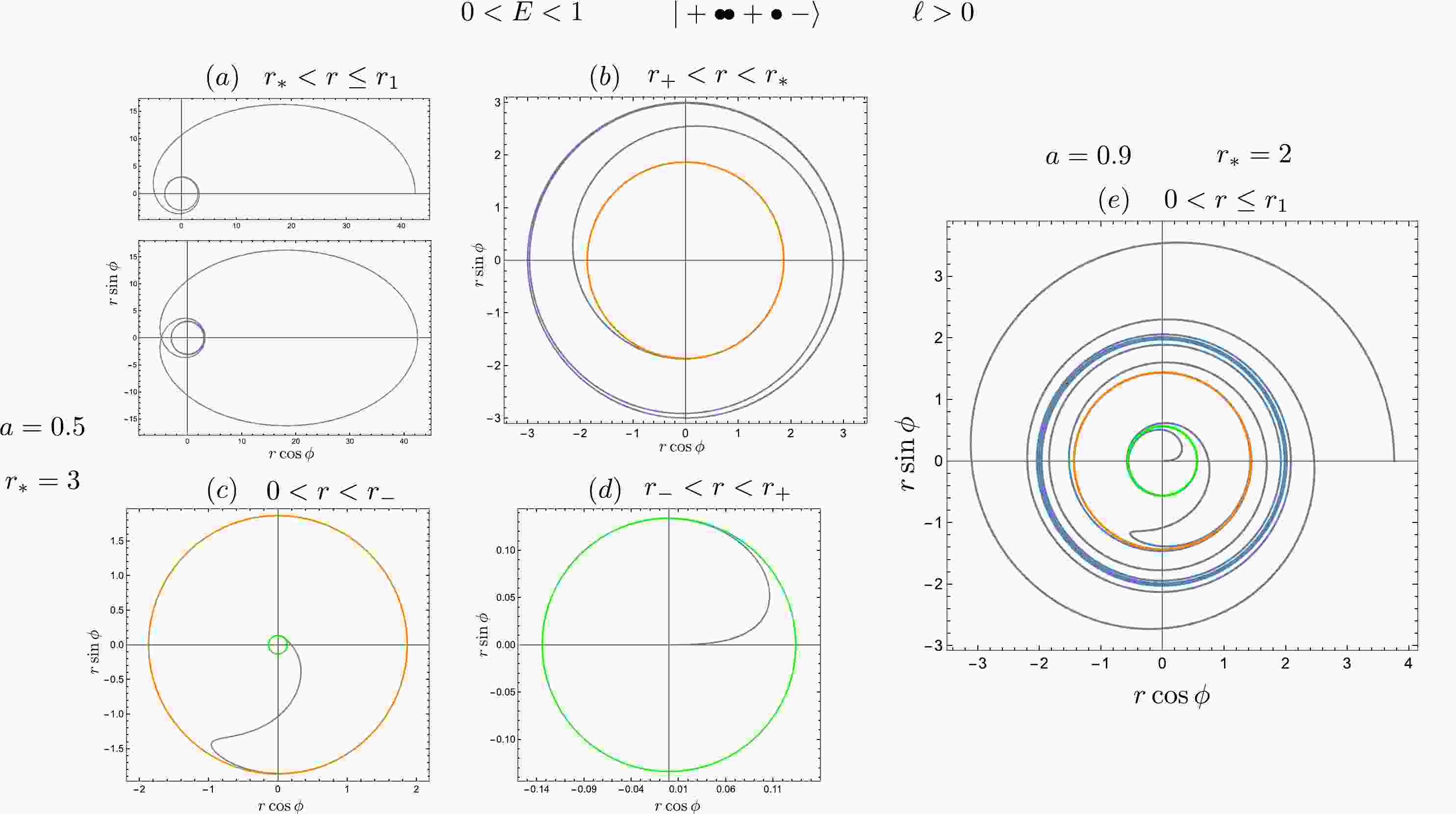
(30) In Fig. 1, we illustrate the geodesics associated with prograde unstable circular orbits, where
$ 0<E<1 $ . The behavior of different orbit classes in various regions is shown separately in plots$ (a) $ to$ (d) $ . Plot$ (a) $ demonstrates the behavior of ingoing and outgoing-to-ingoing homoclinic orbits confined within the region$ r_*<r\leq r_1 $ , which asymptotically approach the unstable circular orbits. This is consistent with previous findings [25]. Plot$ (b) $ depicts a trapped orbit that originates from the unstable circular orbits and eventually plunges into the black hole. Plots$ (c) $ and$ (d) $ illustrate the trajectories from$ r_+ $ to$ r_- $ and from$ r_- $ to$ 0 $ , respectively. Notably, the direction of motion changes at the horizons owing to the presence of$ \Delta(r) $ in the denominator of$ U^\phi $ , despite the conserved energy and angular momentum remaining constant. Finally, in plot$ (e) $ , we present the entire range of geodesics, choosing$ a=0.9 $ to ensure visibility inside the horizon.
Figure 1. (color online) Geodesics associated with unstable prograde circular orbits. The blue, orange, and green lines represent the orbit, outer horizon, and inner horizon, respectively. The color scheme remains consistent throughout the subsequent figures.
In Fig. 2, we present the geodesics related to the retrograde unstable circular orbits with energy
$ 0<E<1 $ . Plot$ (b) $ shows an interesting phenomenon: near the horizon, the strong gravity drags the retrograde trajectory to become prograde. As a result, the location of the turning point of the ϕ motion outside the horizon,
Figure 2. (color online) Geodesics related to the unstable retrograde circular orbits with the root structure
$ \vert+\bullet\bullet+\bullet-\rangle $ .$ r_{\phi T}=2+\frac{2aE}{\ell}, $

(31) depends on the position of the circular orbits
$ r_* $ and the spin of the black hole a, which can be obtained by solving$ \dfrac{ {\rm{d}}\phi}{ {\rm{d}} r}=0 $ .Notably, (31) is applicable to circular orbits and other retrograde trapped orbits, including those associated with bound or deflecting orbits or purely trapped orbits with the root structure
$ \vert+\bullet -\rangle $ . By inputting the corresponding energy and angular momentum values, one can obtain explicit expressions for these orbits as well. -
When
$ E>1 $ , the circular orbits are unstable with the root structure$ \vert+\bullet\bullet+\rangle $ . The orbits in the first$ + $ region are the whirling trapped orbits, and those in the second$ + $ region are whirling deflecting orbits.For the
$ \mathcal{W} \mathcal{T}^u $ related to the unstable circular orbits in the region$ r_+<r<r_* $ and the orbits inside the horizon$ 0<r<r_+ $ , the ingoing radial velocity is given by$ U^r=\frac{ {\rm{d}} r}{ {\rm{d}}\tau}=-\frac{(r_*-r)\sqrt{(E^2-1)r(r-r_1)}}{r^2}. $

(32) In the region
$ r>r_* $ , the radial velocity for the$ \mathcal{W} \mathcal{D}^u $ is given by$ U^r=\frac{ {\rm{d}} r}{ {\rm{d}}\tau}=-\frac{(r-r_*)\sqrt{(E^2-1)r(r-r_1)}}{r^2}. $

(33) After the integration in the corresponding region, we obtain the proper time of the orbits in the region
$ r<r_* $ $ \begin{aligned}[b] -\sqrt{1-E^2}\tau=\;&\frac{2r_*^{3/2}}{\sqrt{r_*-r_1}}\tanh^{-1}\sqrt{\frac{r(r_*-r_1)}{r_*(r-r_1)}}\\&-(r_1+2r_*)\sinh^{-1}\sqrt{\frac{r}{-r_1}}-\sqrt{r(r-r_1)}, \end{aligned} $

(34) and in the region
$ r>r_* $ $ \begin{aligned}[b] \sqrt{1-E^2}\tau=\;&\frac{2r_*^{3/2}}{\sqrt{r_*-r_1}}\tanh^{-1}\sqrt{\frac{r_*(r-r_1)}{r(r_*-r_1)}}\\&-(r_1+2r_*)\sinh^{-1}\sqrt{\frac{r}{-r_1}}-\sqrt{r(r-r_1)}. \end{aligned} $

(35) The ϕ motion can be obtained by integrating (17) in the corresponding region as follows:
● whirling trapped orbits in the region
$ r_+<r<r_* $ ,$ \begin{aligned}[b] \phi=\;&C_*^2\tanh^{-1}\sqrt{\frac{r(r_*-r_1)}{r_*(r-r_1)}}+C_-^2\tanh^{-1}\sqrt{\frac{r_-(r-r_1)}{r({r\_{} -}r_1)}}\\&+C_+^2\tanh^{-1}\sqrt{\frac{r_+(r-r_1)}{r(r_+-r_1)}}, \end{aligned} $

(36) ● whirling deflecting orbits in the region
$ r>r_* $ ,$ \begin{aligned}[b] \phi=\;&-C_*^2\tanh^{-1}\sqrt{\frac{r_*(r-r_1)}{r(r_*-r_1)}}-C_-^2\tanh^{-1}\sqrt{\frac{r_-(r-r_1)}{r(r\_-r_1)}}\\&-C_+^2\tanh^{-1}\sqrt{\frac{r_+(r-r_1)}{r(r_+-r_1)}}, \end{aligned} $

(37) ● orbits in the region
$ r_-<r<r_+ $ ,$ \begin{aligned}[b] \phi=\;&C_*^2\tanh^{-1}\sqrt{\frac{r(r_*-r_1)}{r_*(r-r_1)}}+C_-^2\tanh^{-1}\sqrt{\frac{r_-(r-r_1)}{r(r\_-r_1)}}\\&+C_+^2\tanh^{-1}\sqrt{\frac{r(r_+-r_1)}{r_+(r-r_1)}}, \end{aligned} $

(38) ● orbits in the region
$ 0<r<r_- $ ,$ \begin{aligned}[b] \phi=\;&C_*^2\tanh^{-1}\sqrt{\frac{r(r_*-r_1)}{r_*(r-r_1)}}+C_-^2\tanh^{-1}\sqrt{\frac{r(r\_-r_1)}{r_-(r-r_1)}}\\&+C_+^2\tanh^{-1}\sqrt{\frac{r(r_+-r_1)}{r_+(r-r_1)}}, \end{aligned} $

(39) where the constants are given by
$ C_*^2=\frac{2\sqrt{r_*}(2(\ell-aE)-r_*\ell)}{\sqrt{1-E^2}\sqrt{r_*-r_1}(r_*-r_-)(r_*-r_+)}, $

(40) $ C_-^2=\frac{2\sqrt{r_-}(2(\ell-aE)-r_-\ell)}{\sqrt{1-E^2}\sqrt{r_- - r_1}(r_*-r_-)(r_+ - r_-)}, $

(41) $ C_-^2=\frac{2\sqrt{r_+}(2(\ell-aE)-r_+\ell)}{\sqrt{1-E^2}\sqrt{r_+-r_1}(r_*-r_-)(r_- - r_+)}. $

(42) In Fig. 3 and Fig. 4, we illustrate the geodesics associated with the prograde and retrograde unstable circular orbits with energy
$ E>1 $ . Plots$ (a) $ to$ (d) $ display the distinct classes of orbits, where$ a=0.5 $ and$ r_*=3 $ . Additionally, plot$ (e) $ showcases all classes of orbits within the root structure$ \vert+\bullet\bullet +\rangle $ , with$ a=0.9 $ and$ r_*=4 $ . Notably, plots$ (a) $ demonstrate the whirling deflecting orbits originating from far infinity and asymptotically approaching the unstable circular orbits. The turning points of the trapped retrograde orbits, located at$ r=r_{\phi T} $ , are also evident.
Figure 3. (color online) Geodesics related to the unstable prograde circular orbits with
$ E>1 $ .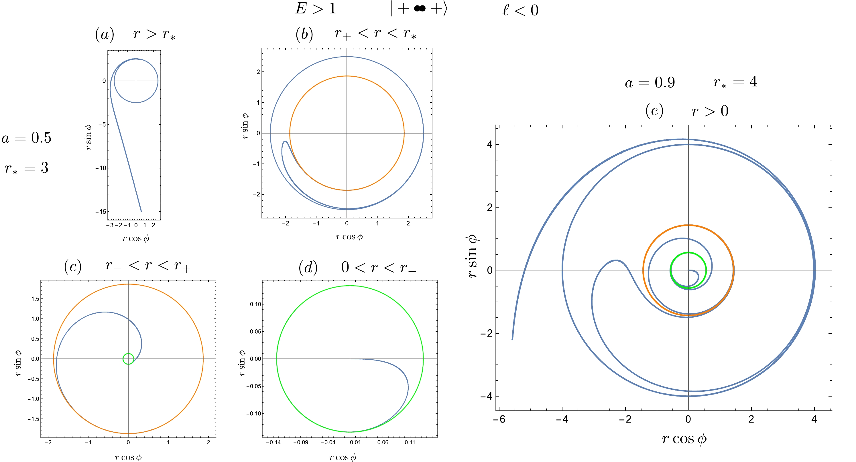
Figure 4. (color online) Geodesics related to the unstable retrograde circular orbits with
$ E>1 $ . -
We now discuss the ingoing trapped orbits with the root structure
$ \vert+\bullet-\bullet\bullet-\rangle $ . These orbits are characterized by having energy values confined in the region$ E_{I^\pm}<E<1 $ and stable circular orbits located at$ r_*>r_{I^\pm} $ . Notably, when$ r_{1^+}=r_+ $ , the single root touches the horizon, and the stable circular orbit is located at$ r_*=r^s_+=\frac{4r_+}{a^2}+2\sqrt{3+r_+ +\frac{8r_+}{a^4}-\frac{4(2r_+ +1)}{a^2}}-r_+ -2. $

(43) At this point, the angular momentum and energy are given by
$ \ell=\ell^{(1)}=\ell_+, $

(44) $ E=E^{(1)}=\frac{a\ell^{(1)}}{2r_+}. $

(45) When
$ r_*>r^s_+ $ , the angular momentum is greater than$ \ell_+ $ , indicating that, although the stable circular orbits exist, the trapped orbits are disallowed. However, the trapped orbits exist for the orbital motion with negative energy even though the related circular orbits are disallowed. In this scenario, we can employ the parameters of the circular orbits to investigate the motion with negative energy, taking advantage of the symmetry in$ R(r) $ achieved by flipping the sign of E and$ \ell $ simultaneously.Based on the analysis above, we can draw the following conclusions regarding the existence of trapped orbits:
● For prograde orbits, the trapped orbits exist within the range
$ r_c^{(1)}<r_*<r_+^s $ .● For retrograde orbits, the trapped orbits exist when
$ r_*>r_c^{(2)} $ .● For orbits with negative energy, the trapped orbits exist when
$ r_*>r^s_+ $ .These findings offer valuable insights into the critical role of
$ r_* $ in determining the presence of trapped orbits alongside the associated stable circular orbits. These insights are particularly useful when plotting the trajectories of these trapped orbits. To ensure the existence of trapped orbits, it is crucial to carefully select appropriate values for$ r_* $ . Thus, one can accurately depict the trajectories and study the characteristics of these intriguing orbits.For the trapped orbits related to the stable circular orbits, which represent the allowed motion in the
$ + $ region$ r_+<r<r_1<r_* $ of the root structure, as well as the orbits inside the horizon, the radial velocity is given by$ U^r=-\frac{(r_*-r)\sqrt{(E^2-1)r(r-r_{1})}}{r^2}. $

(46) By integrating the above expression, we obtain the proper time as
$ \begin{aligned}[b] -\sqrt{1-E^2}\tau=\;&r\sqrt{\frac{r_1}{r}-1}+(r_1+r_*)\arctan\sqrt{\frac{r_1}{r}-1}\\&-\frac{2r_*^{3/2}}{\sqrt{r_*-r_1}}\arctan\sqrt{\frac{r_*(r_1-r)}{r(r_*-r_1)}}. \end{aligned} $

(47) For the azimuthal motion, we have the following expressions:
● trapped orbits in the region
$ r_+<r\leq r_1 $ ,$ \begin{aligned}[b] \phi=\;&-C_*^2\arctan\sqrt{\frac{r_*(r_1-r)}{r(r_*-r_1)}}+C_-^1\tanh^{-1}\sqrt{\frac{r_-(r_1-r)}{r(r_1-r_-)}}\\&+C_+^1\tanh^{-1}\sqrt{\frac{r_+(r_1-r)}{r(r_1-r_+)}}. \end{aligned} $

(48) ● the motion in the region
$ r_-<r<r_+ $ ,$ \begin{aligned}[b] \phi=\;&-C_*^2\arctan\sqrt{\frac{r_*(r_1-r)}{r(r_*-r_1)}}+C_-^1\tanh^{-1}\sqrt{\frac{r_-(r_1-r)}{r(r_1-r_-)}}\\&+C_+^1\tanh^{-1}\sqrt{\frac{r(r_1-r_+)}{r_+(r_1-r)}}. \end{aligned} $

(49) ● the motion in the region
$ 0<r<r_- $ ,$ \begin{aligned}[b] \phi=\;&-C_*^2\arctan\sqrt{\frac{r_*(r_1-r)}{r(r_*-r_1)}}+C_-^1\tanh^{-1}\sqrt{\frac{r(r_1-r_-)}{r_-(r_1-r)}}\\&+C_+^1\tanh^{-1}\sqrt{\frac{r(r_1-r_+)}{r_+(r_1-r)}}. \end{aligned} $

(50) In Fig. 5, we present the geodesics in the region
$ 0<r\leq r_1 $ associated with stable circular orbits. Plots$ (a) $ and$ (b) $ display the geodesics related to prograde stable circular orbits with different black hole spins. It indicates that as the black hole rotates faster, the turning point$ r_1 $ approaches closer to the horizon. Plot$ (c) $ illustrates the geodesics related to retrograde stable circular orbits. Notably, for retrograde stable circular orbits,$ r_* $ can go to infinity without affecting the existence of trapped orbits. Finally, plot$ (d) $ showcases the geodesic motion with negative energy. Here, we observe that there are no turning points for the ϕ motion, both inside and outside the black hole. Furthermore, the trajectory remains prograde despite the negative angular momentum. One can check that our results match those in [36] very well by replacing the notations in Eqs. (53)−(54), Eqs. (56)−(57), and Eqs. (61)−(63) from [36] with ours.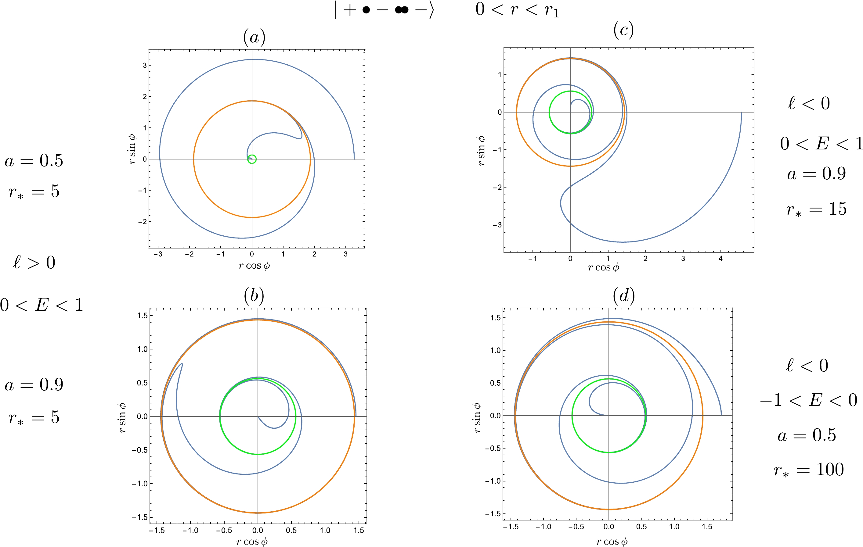
Figure 5. (color online) Geodesics related to the stable circular orbits with the root structure
$ \vert+\bullet-\bullet\bullet-\rangle $ . -
In the region between
$ \ell^s $ and$ \ell^u $ , as shown in Figure 8 of [34], the double root separates into two single roots. These single roots correspond to the turning points of bound orbits when$ E<1 $ , and they represent the turning points of the trapped and deflecting orbits when$ E>1 $ . The separation of these roots, which is described by the separatrix in terms of the semilatus rectum and eccentricity, has been extensively discussed in previous works such as [25, 27, 34, 39, 40]. In this section, we delve into the analysis of trapped orbits associated with these separated roots and explore the properties of deflecting orbits.We first consider the root structure
$ \vert+\bullet-\bullet+\bullet -\rangle $ with bound orbits. The trapped orbits in the first$ + $ region$ r_+<r<r_1 $ are allowed when$ \ell^u<\ell<\min(\ell^s,\ell^+) $ and$ E_I<E<1 $ . When$ \ell>\ell_+ $ , the trapped orbits are disallowed even though the bound orbits exist. Now, we express the radial potential as$ \frac{R(r)}{E^2-1}=(r-r_1)(r-r_p)(r-r_a), $

(51) where the roots of the radial potential
$ r_1<r_p<r_a $ represent the turning points of trapped and bound orbits. Here,$ r_p=\dfrac{p}{1+e} $ and$ r_a=\dfrac{p}{1-e} $ denote the pericenter and apocenter of the bound orbits, respectively, where p is the semilatus rectum, and e is the eccentricity. By comparing the coefficients of r with (1), one can obtain the following solution:$ r_1=\frac{2}{1-E^2}-(r_a+r_p) , $

(52) $ \ell^{(1),(2)}=aE\pm\sqrt{\frac{r_a r_p(2+(E^2-1)(r_a+r_p))}{2}}, $

(53) $ E^{(1),(2)}=\sqrt{\frac{X_1+X_2\pm4\sqrt{2}a\sqrt{r_a r_p(r_a+r_p)\Delta(r_a)\Delta(r_p)}}{X_3+X_4}}, $

(54) where the indices
$ (1) $ and$ (2) $ correspond to the$ + $ and$ - $ sign in$ \pm $ , and$ X_1=(r_a-2)(r_p-2)(r_a+r_p)(r_a(r_a+r_p)(r_p-2)-2r_p^2), $

(55) $ X_2=a^2(r_a^2(4-6r_p)-6r_a r_p(r_p-2)+4r_p^2), $

(56) $ X_3=r_a^3(r_a+2r_p )(r_p-2)^2+4r_p^2(r_p^2-r_a (\Delta(r_p)+a^2)), $

(57) $ X_4=r_a^2 r_p(r_p(r_p-6)(r_p-2)-8a^2). $

(58) Note that we have
$ \ell^{(1)}>0 $ ,$ \ell^{(2)}<0 $ . The allowed branches are as follows: prograde orbits$ (\ell^{(1)}(E^{(2)}),E^{(2)}) $ , retrograde orbits$ (\ell^{(2)}(E^{(1)}),E^{(1)}) $ , and orbits with negative energy$ (\ell^{(2)}(-E^{(2)}),-E^{(2)}) $ .By replacing
$ r_p=\dfrac{p}{1+e} $ and$ r_a=\dfrac{p}{1-e} $ in (51), and comparing the coefficients of r with the radial potential, one can obtain the quantities and the polynomial that the semi-latus rectum and eccentricity should satisfy,$ E=\pm\sqrt{1+\frac{2(e^2-1)}{2p+r_1(1-e^2)}} , $

(59) $ \ell=aE\pm p\sqrt{\frac{r_1}{2p+(1-e^2)r_1}} , $

(60) $ \begin{aligned}[b] 0=\;&\{p[4r_1-p(r_1-2)]-a^2[2p+r_1(1-e^2)]\}^2{}\\ &-4a^2 p^2 r_1[r_1+2(p-1)-e^2(r_1-2)]. \end{aligned} $

(61) For trapped and deflecting orbits with the root structure
$ \vert+\bullet-\bullet +\rangle $ ,$ r_a $ is negative such that it is no longer the apocenter, which we denote by$ r_n $ , and$ r_p $ is no longer the pericenter but the turning point of the deflecting orbits, denoted by$ r_d $ . Note that we still have$ r_n=\dfrac{p}{1-e} $ and$ r_d=\dfrac{p}{1+e} $ , and$ e>1 $ is no longer the eccentricity. The other single root$ r_1 $ and the energy and angular momentum of the orbits can be obtained by simply replacing$ r_a $ and$ r_p $ with$ r_n $ and$ r_d $ , respectively, in (52)−(54). -
The radial velocity of the trapped orbit associated with a bound orbit is given by
$ U^r=-\frac{\sqrt{(E^2-1)r(r-r_1)(r-r_p)(r-r_a)}}{r^2}, $

(62) which can be rewritten as
$ -\sqrt{(1-E^2)} {\rm{d}}\tau=\frac{1}{\sqrt{\left(\dfrac{r_1}{r}-1\right)\left(\dfrac{r_p}{r}-1\right)\left(\dfrac{r_a}{r}-1\right)}} {\rm{d}} r. $

(63) Let
$ \dfrac{r}{r_a}=\sin^2\psi $ ,$ \dfrac{r_1}{r_a}=\sin^2\psi_1 $ , and$ \dfrac{r_p}{r_a}=\sin^2\psi_p $ . Then, reverting the substitution after the integration, we obtain the expression for the proper time,$\begin{aligned}[b] \frac{-\sqrt{1-E^2}}{r_a}\tau=\frac{\sqrt{r_p(r_a-r_1)}}{r_a} \mathcal{E}\left(\arcsin\left(\sqrt{\frac{r(r_1-r_a)}{r_1(r-r_a)}}\right)\Bigg|\frac{r_1(r_p-r_a)}{r_p(r_1-r_a)}\right)\end{aligned} $

(64) $ \quad\quad\quad\quad\quad +\frac{r_1+r_a}{\sqrt{r_p(r_a-r_1)}} \mathcal{F}\left(\arcsin\left(\sqrt{\frac{r(r_1-r_a)}{r_1(r-r_a)}}\right)\Bigg|\frac{r_1(r_p-r_a)}{r_p(r_1-r_a)}\right) $

(65) $\quad\quad\quad \quad\quad-\frac{r_1+r_a+r_p}{\sqrt{r_p(r_a-r_1)}}\Pi\left(\frac{r_1}{r_1-r_a};\arcsin\left(\sqrt{\frac{r(r_1-r_a)}{r_1(r-r_a)}}\right)\Bigg|\frac{r_1(r_p-r_a)}{r_p(r_1-r_a)}\right) $

(66) $\quad\quad\quad\quad\quad +\sqrt{\frac{r(r_1-r)(r_p-r)}{r_a^2(r_a-r)}}, $

(67) where
$ \mathcal{F}(x|c) $ is the elliptic integral of the first kind,$ \mathcal{E}(x|c) $ is the elliptic integral of the second kind, and$ \Pi(n;x|c) $ is the incomplete elliptic integral of the third kind, which are defined in Appendix A.Similarly, let
$ \dfrac{r_+}{r_a}=\sin^2\psi_+ $ and$ \dfrac{r_-}{r_a}=\sin^2\psi_- $ ; reverting the substitution after the integration, we obtain the solution of the azimuthal motion,$ \begin{aligned}[b] \phi=\;&\frac{2r_a}{\sqrt{1-E^2}\sqrt{r_1(r_a-r_p)}}\left(\frac{2(\ell-aE)-r_a\ell}{(r_a-r_-)(r_a-r_+)} \mathcal{F}\left(\arcsin\left(\sqrt{\frac{r(r_p-r_a)}{r_p(r-r_a)}}\right)\Bigg|\frac{r_p(r_a-r_1)}{r_1(r_a-r_p)}\right)\right.{}\\ &-\frac{2(\ell-aE)-r_-\ell}{(r_a-r_-)(r_+-r_-)}\Pi\left(\frac{r_p(r_a-r_-)}{r_-(r_a-r_p)};\arcsin\left(\sqrt{\frac{r(r_p-r_a)}{r_p(r-r_a)}}\right)\Bigg|\frac{r_p(r_a-r_1)}{r_1(r_a-r_p)}\right){}\\ &\left.-\frac{2(\ell-aE)-r_+\ell}{(r_a-r_+)(r_+-r_-)}\Pi\left(\frac{r_p(r_a-r_+)}{r_+(r_a-r_p)};\arcsin\left(\sqrt{\frac{r(r_p-r_a)}{r_p(r-r_a)}}\right)\Bigg|\frac{r_p(r_a-r_1)}{r_1(r_a-r_p)}\right)\right). \end{aligned} $

(68) Noticing that a symmetry exists by exchanging
$ r_1 $ and$ r_p $ in (63) and with the replacements below (63), one can easily obtain another equivalent solution as$ \begin{aligned}[b] \phi=\;&\frac{2r_a}{\sqrt{1-E^2}\sqrt{r_p(r_a-r_1)}}\left(\frac{2(\ell-aE)-r_a\ell}{(r_a-r_-)(r_a-r_+)} \mathcal{F}\left(\arcsin\left(\sqrt{\frac{r(r_1-r_a)}{r_1(r-r_a)}}\right)\Bigg|\frac{r_1(r_a-r_p)}{r_p(r_a-r_1)}\right)\right.{}\\ &-\frac{2(\ell-aE)-r_-\ell}{(r_a-r_-)(r_+-r_-)}\Pi\left(\frac{r_1(r_a-r_-)}{r_-(r_a-r_1)};\arcsin\left(\sqrt{\frac{r(r_1-r_a)}{r_1(r-r_a)}}\right)\Bigg|\frac{r_1(r_a-r_p)}{r_p(r_a-r_1)}\right){}\\ &\left.-\frac{2(\ell-aE)-r_+\ell}{(r_a-r_+)(r_+-r_-)}\Pi\left(\frac{r_1(r_a-r_+)}{r_+(r_a-r_1)};\arcsin\left(\sqrt{\frac{r(r_1-r_a)}{r_1(r-r_a)}}\right)\Bigg|\frac{r_1(r_a-r_p)}{r_p(r_a-r_1)}\right)\right). \end{aligned} $

(69) Note that this solution also applies to the orbits inside the horizon.
In Fig. 6, we illustrate the behavior of the trapped orbits, which exhibit similarities with the trapped orbits related to circular orbits.

Figure 6. (color online) Geodesics related to the bound orbits with the root structure
$ \vert+\bullet-\bullet+\bullet- \rangle $ . -
The trapped orbits is confined in the first
$ + $ region of the root structure$ \vert+\bullet-\bullet +\rangle $ , where we have$ r_n<0<r_+<r<r_1<r_d<-r_n $ . Setting$ \dfrac{r}{-r_n}=\sin^2\psi $ ,$ \dfrac{r_1}{-r_n}=\sin^2\psi_1 $ , and$ \dfrac{r_d}{-r_n}=\sin^2\psi_d $ , we have$ -\sqrt{E^2-1} {\rm{d}}\tau=\frac{\sin2\psi}{\sqrt{(1+\csc^2\psi)(\csc^2\psi\sin^2\psi_1-1)(\csc^2\psi\sin^2\psi_1-1)}} {\rm{d}}\psi, $

(70) let
$ x=\csc\psi $ , and replace back after the integration, we obtain the proper time expressed as$ \frac{-\sqrt{E^2-1}}{(-r_n)}\tau=C_ \mathcal{E} \mathcal{E}\left(\arcsin\left(\sqrt{\frac{(r-r_n)(r_n+r_d)}{(r+r_n)(r_d-r_n)}}\right)\Bigg|\frac{(r_1+r_n)(r_d-r_n)}{(r_d+r_n)(r_1-r_n)}\right) $

(71) $ \quad\quad\quad\quad\quad +C_ \mathcal{F} \mathcal{F}\left(\arcsin\left(\sqrt{\frac{(r-r_n)(r_n+r_d)}{(r+r_n)(r_d-r_n)}}\right)\Bigg|\frac{(r_1+r_n)(r_d-r_n)}{(r_d+r_n)(r_1-r_n)}\right), $

(72) $ \quad\quad\quad\quad\quad +C_\Pi\Pi\left(\frac{r_d-r_n}{r_n+r_d};\arcsin\left(\sqrt{\frac{(r-r_n)(r_n+r_d)}{(r+r_n)(r_d-r_n)}}\right)\Bigg|\frac{(r_1+r_n)(r_d-r_n)}{(r_d+r_n)(r_1-r_n)}\right) $

(73) $ \quad\quad\quad\quad\quad +\frac{\sqrt{(r-r_1)(r_n^2-r_1^2)(r-r_d)}}{2r_n(r+r_n)}. $

(74) where
$ C_ \mathcal{E}=\frac{\sqrt{(r_n-r_1)(r_n+r_d)}}{-2r_n}, $

(75) $ C_ \mathcal{F}=\frac{r_d}{\sqrt{(r_n-r_1)(r_n+r_d)}}, $

(76) $ C_\Pi=\frac{-(r_1+r_d)}{\sqrt{(r_n-r_1)(r_n+r_d)}}. $

(77) Similarly, we obtain the solution of the ϕ motion as
$ \begin{aligned}[b] \phi=\;&\frac{2r_n(2(\ell-aE)-r_n\ell)}{\sqrt{(E^2-1)(r_1-r_n)r_d}(r_n-r_-)(r_n-r_+)} \mathcal{F}\left(\arcsin\left(\sqrt{\frac{r(r_1-r_n)}{r_1(r-r_n)}}\right)\Bigg|\frac{r_1(r_d-r_n)}{(r_1-r_n)r_d}\right){}\\ &-\frac{2r_n(2(\ell-aE)-r_-\ell)}{\sqrt{(E^2-1)(r_1-r_n)r_d}(r_n-r_-)(r_- -r_+)}\Pi\left(\frac{r_1(r_- -r_n)}{r_-(r_1-r_n)};\arcsin\left(\sqrt{\frac{r(r_1-r_n)}{r_1(r-r_n)}}\right)\Bigg|\frac{r_1(r_d-r_n)}{(r_1-r_n)r_d}\right){}\\ &-\frac{2r_n(2(\ell-aE)-r_+\ell)}{\sqrt{(E^2-1)(r_1-r_n)r_d}(r_+-r_-)(r_n -r_+)}\Pi\left(\frac{r_1(r_+ -r_n)}{r_+(r_1-r_n)};\arcsin\left(\sqrt{\frac{r(r_1-r_n)}{r_1(r-r_n)}}\right)\Bigg|\frac{r_1(r_d-r_n)}{(r_1-r_n)r_d}\right).{}\\ \end{aligned} $

(78) Note that the behavior of the trapped trajectory in this region is similar to the one depicted in Fig. 6.
-
For the deflecting orbits in the second
$ + $ region from the second turning point to infinity, the redial velocity can be rewritten as$ -\sqrt{E^2-1} {\rm{d}}\tau=\frac{1}{\sqrt{\left(1-\dfrac{r_1}{r}\right)\left(1-\dfrac{r_n}{r}\right)\left(1-\dfrac{r_d}{r}\right)}} {\rm{d}} r. $

(79) After the integration, we obtain the proper time expressed as
$ \begin{aligned}[b] -\sqrt{E^2-1}\tau=\;&\sqrt{\frac{r(r-r_n)(r-r_d)}{r-r_1}}- \mathcal{E}\left(\arcsin\left(\sqrt{\frac{(r_n-r_1)(r-r_d)}{(r-r_1)(r_n-r_d)}}\right)\Bigg|\frac{r_1(r_d-r_n)}{r_d(r_1-r_n)}\right){}\\ &+\sqrt{\frac{1}{r_d(r_1-r_n)}}(r_1 (r_1 + r_n) + (r_1 - r_n) r_d) \mathcal{F}\left(\arcsin\left(\sqrt{\frac{(r_n-r_1)(r-r_d)}{(r-r_1)(r_n-r_d)}}\right)\Bigg|\frac{r_1(r_d-r_n)}{r_d(r_1-r_n)}\right){}\\ &-\sqrt{\frac{1}{r_d(r_1-r_n)}}(r_1 - r_d) (r_1 + r_n + r_d)\Pi\left(\frac{r_d-r_a}{r_1-r_n};\arcsin\left(\sqrt{\frac{(r_n-r_1)(r-r_d)}{(r-r_1)(r_n-r_d)}}\right)\Bigg|\frac{r_1(r_d-r_n)}{r_d(r_1-r_n)}\right){} .\\ \end{aligned} $ 
(80) For the ϕ motion, we have
$ \phi=\frac{2(\ell-aE)I_1^d-\ell I_2^d}{\sqrt{E^2-1}}, $

(81) where
$ I^d_j=\int\frac{r^{j-1}}{\sqrt{\dfrac{(r-r_1)(r-r_n)(r-r_d)}{r}}(r-r_-)(r-r_+)} {\rm{d}} r . $

(82) After the integration, we obtain the solution of the azimuthal motion,
$ \begin{aligned}[b] \phi=\;&\frac{2(r_1-r_d)}{\sqrt{E^2-1}\sqrt{(r_1-r_n)r_d}}\left(\frac{2(\ell-aE)r_1-\ell r_1^2}{(r_1 - r_d) (r_1 - r_-) (r_1 - r_+)} \mathcal{F}\left(\arcsin\left(\sqrt{\frac{(r_n-r_1)(r-r_d)}{(r-r_1)(r_n-r_d)}}\right)\Bigg|\frac{r_1(r_d-r_n)}{r_d(r_1-r_n)}\right)\right.{}\\ &-\frac{2(\ell-aE)r_- -\ell r_-^2}{(r_- - r_d) (r_1 - r_-) (r_- - r_+)}\Pi\left(\frac{(r_d-r_n)(r_1-r_-)}{(r_1-r_n)(r_d-r_-)};\arcsin\left(\sqrt{\frac{(r_n-r_1)(r-r_d)}{(r-r_1)(r_n-r_d)}}\right)\Bigg|\frac{r_1(r_d-r_n)}{r_d(r_1-r_n)}\right){}\\ &\left.-\frac{2(\ell-aE)r_+-\ell r_+^2}{(r_+ - r_d) (r_1 - r_+) (r_+ - r_-)}\Pi\left(\frac{(r_d-r_n)(r_1-r_+)}{(r_1-r_n)(r_d-r_+)};\arcsin\left(\sqrt{\frac{(r_n-r_1)(r-r_d)}{(r-r_1)(r_n-r_d)}}\right)\Bigg|\frac{r_1(r_d-r_n)}{r_d(r_1-r_n)}\right)\right).{}\\ \end{aligned} $

(83) In Fig. 7, we depict the trajectory of deflecting orbits. An intriguing characteristic of these trajectories is that, as the turning point approaches the turning point of the corresponding trapped orbits, the particle completes more revolutions around the black hole. When these two turning points merge into a double root, the orbit transforms into a whirling deflecting orbit, which asymptotically converges to the unstable circular orbit illustrated in Fig. 4. Consequently, no outgoing trajectories are observed.
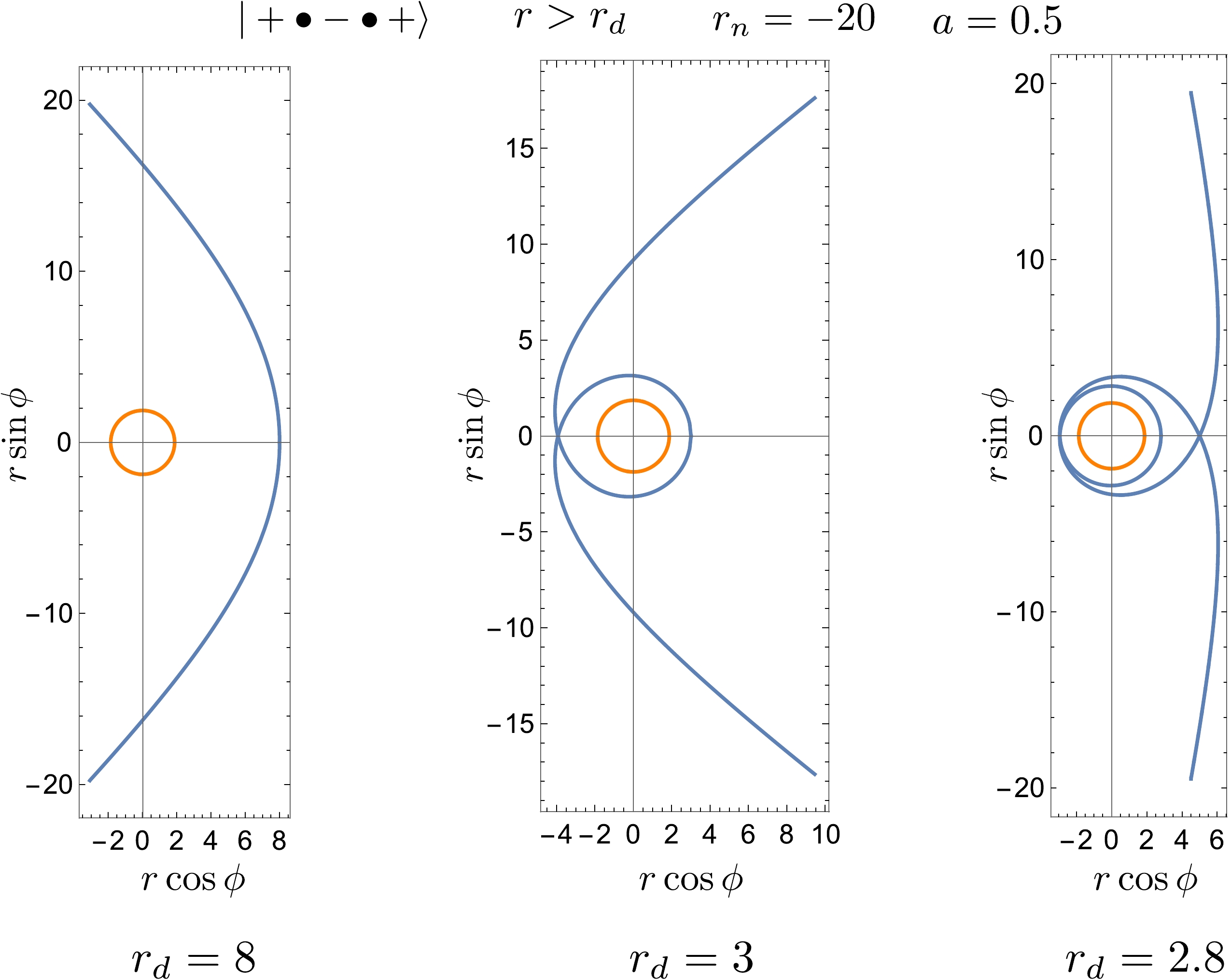
Figure 7. (color online) Deflecting orbits with the root structure
$ \vert+\bullet-\bullet +\rangle $ . -
For the radial potential of marginal orbits with
$ E=1 $ , one root goes to infinity; then, the radial potential is reduced to$ \begin{array}{*{20}{l}} R_1=2r^2-\ell^2r+2(a-\ell)^2. \end{array} $

(84) The circular orbits locate at
$ r_*=r_c^{(1),(2)} $ in the root structure$ \vert+\bullet\bullet+\rangle $ , with the angular momentum$ \begin{array}{*{20}{l}} \ell_{M*}^{(1),(2)}=\pm2(1+\sqrt{1\mp a}), \end{array} $

(85) the radial velocity is expressed as
$ U^r=\frac{ {\rm{d}} r}{ {\rm{d}}\tau}=\pm\frac{\sqrt{2r(r-r_*)^2}}{r^2}. $

(86) For the root structure
$ \vert+\bullet-\bullet +\rangle $ with the trapped and deflecting orbits, the turning point of the trapped orbit locates at$ r_1=\dfrac{\ell^2}{2}-r_d $ , where the angular momentum is$ \ell_{MD}^{(1),(2)}=\frac{-2a\pm\sqrt{2r_d\Delta(r_d)}}{r_d-2}, $

(87) and the radial velocity is expressed as
$ U^r=\frac{ {\rm{d}} r}{ {\rm{d}}\tau}=\pm\frac{\sqrt{2r(r-r_1)(r-r_d)}}{r^2}. $

(88) When the second turning point locates at the ergosphere, i.e.,
$ r_d=2 $ , we have$ r_1=\frac{(a^2-4)^2}{8a^2}, \quad\ell=\frac{2}{a}+\frac{a}{2}. $

(89) Note that, when
$ r_d>2 $ , we have$ \ell_{MD}^{(1)}>0 $ and$ \ell_{MD}^{(2)}<0 $ ; when$ r_+<r_d<2 $ , we have$ \ell_{MD}^{(1),(2)}>0 $ , which means that, inside the ergoregion, only the prograde marginal deflecting orbits exist. Note that, when$ E=-1 $ , the angular momentum is$ -\ell_{MD}^{(1)} $ . -
For the whirling trapped orbits in the first
$ + $ region of the root structure$ \vert+\bullet\bullet+\rangle $ ,$ -\sqrt{2} {\rm{d}}\tau=\frac{\sqrt{r}}{\dfrac{r_*}{r}-1} {\rm{d}} r, $

(90) and after the integration, we obtain
$ -\sqrt{2}\tau=2r_*^{3/2}\tanh^{-1}\sqrt{\frac{r}{r_*}}-\frac{2}{3}\sqrt{r}(r+3r_*). $

(91) For the whirling deflecting orbits in the second
$ + $ region of the root structure$ \vert+\bullet\bullet+\rangle $ ,$ -\sqrt{2} {\rm{d}}\tau=\frac{\sqrt{r}}{1-\dfrac{r_*}{r}} {\rm{d}} r, $

(92) and then,
$ -\sqrt{2}\tau=-2r_*^{3/2}\tanh^{-1}\sqrt{\frac{r_*}{r}}+\frac{2}{3}\sqrt{r}(r+3r_*). $

(93) The explicit expressions for the ϕ motion are given as follows:
● whirling trapped orbits in the region
$ r_+<r<r_* $ ,$ \phi=C_*\tanh^{-1}\sqrt{\frac{r}{r_*}}+C_-\tanh^{-1}\sqrt{\frac{r_-}{r}}+C_+\tanh^{-1}\sqrt{\frac{r_+}{r}}, $

(94) ● whirling deflecting orbits in the region
$ r>r_* $ ,$ \phi=-C_*\tanh^{-1}\sqrt{\frac{r_*}{r}}-C_-\tanh^{-1}\sqrt{\frac{r_-}{r}}-C_+\tanh^{-1}\sqrt{\frac{r_+}{r}}, $

(95) ● the orbits in the region
$ r_-<r<r_+ $ ,$ \phi=C_*\tanh^{-1}\sqrt{\frac{r}{r_*}}+C_-\tanh^{-1}\sqrt{\frac{r_-}{r}}+C_+\tanh^{-1}\sqrt{\frac{r}{r_+}}, $

(96) ● the orbits in the region
$ 0<r<r_- $ ,$ \phi=C_*\tanh^{-1}\sqrt{\frac{r}{r_*}}+C_-\tanh^{-1}\sqrt{\frac{r}{r_-}}+C_+\tanh^{-1}\sqrt{\frac{r}{r_+}}, $

(97) where
$ C_*=\frac{\sqrt{r_*}(2(\ell-a)-r_*\ell)}{\sqrt{2}(r_- - r_*)(r_+-r_*)}, $

(98) $ C_-=\frac{\sqrt{r_-}(2(\ell-a)-r_-\ell)}{\sqrt{2}(r_+-r_-)(r_*-r_-)}, $

(99) $ C_+=\frac{\sqrt{r_+}(2(\ell-a)-r_+\ell)}{\sqrt{2}(r_+-r_-)(r_+-r_*)}. $

(100) -
When the angular momentum
$ |\ell|>\ell_{M*}^{(1)} $ or$ \ell<\ell_{M*}^{(2)} $ , the root structure is$ \vert+\bullet-\bullet +\rangle $ . Note that, similar to the non-marginal deflecting orbits, when$ E=1 $ and$ \ell_{M*}^{(1)}<\ell<\ell_+ $ or$ \ell<\ell_{M*}^{(2)} $ , both trapped and deflecting orbits exist; when$ E=1 $ and$ \ell>\ell_+ $ , the trapped orbits are disallowed although the deflecting orbits exist; and when$ E=-1 $ and$ \ell<\ell_+ $ , the trapped orbits are allowed although the deflecting orbits do not exist.For the trapped orbits in the first
$ + $ region of the root structure$ \vert+\bullet-\bullet+\rangle $ ,$ 0<r<r_1<r_d $ ; let$ \dfrac{r}{r_d}=x^2 $ , and we obtain the proper time expressed as$ \begin{aligned}[b] \tau=\;&-\frac{\sqrt{2}}{3}\left(\sqrt{r(r_1-r)(r_d-r)}\right.\\&-2\sqrt{r_1}(r_1+r_d) \mathcal{E}\left(\arcsin\sqrt{\frac{r}{r_d}}\Bigg|\frac{r_d}{r_1}\right){}\\ &\left.+\sqrt{r_1}(2r_1+r_d) \mathcal{F}\left(\arcsin\sqrt{\frac{r}{r_d}}\Bigg|\frac{r_d}{r_1}\right)\right). \end{aligned} $

(101) The ϕ motion for trapped orbits is expressed as
$ \begin{aligned}[b] \phi=\;&-\sqrt{\frac{2}{r_d}}\ell \mathcal{F}\left(\arcsin\sqrt{\frac{r}{r_1}}\Bigg|\frac{r_1}{r_d}\right)\\&+\frac{\sqrt{2}(2a+\ell(r_- -2))}{\sqrt{r_d}(r_ - - r_+)}\Pi\left(\frac{r_1}{r_-};\arcsin\sqrt{\frac{r}{r_1}}\Bigg|\frac{r_1}{r_d}\right){}\\ &-\frac{\sqrt{2}(2a+\ell(r_+-2))}{\sqrt{r_d}(r_- - r_+)}\Pi\left(\frac{r_1}{r_+};\arcsin\sqrt{\frac{r}{r_1}}\Bigg|\frac{r_1}{r_d}\right). \end{aligned} $

(102) For the deflecting orbits in the second
$ + $ region of the root structure$ \vert+\bullet-\bullet+\rangle $ , we introduce$ \dfrac{r_1}{r}=\sin\psi $ and$ \dfrac{r_1}{r_d}=\sin\psi_1 $ to confine the variables in the deflecting region. Then, we obtain the proper time expressed as$ \begin{aligned}[b] -\tau=\;&\frac{\sqrt{2}}{3r}\sqrt{r(r-r_1)(r-r_d)}(r+2(r_1+r_d)){}\\ &+\frac{2\sqrt{2}}{3}\sqrt{r_1}(r_1+r_d) \mathcal{E}\left(\arcsin\sqrt{\frac{r_1}{r}}\Bigg|\frac{r_d}{r_1}\right){}\\ &-\frac{\sqrt{2}}{3}\sqrt{r_1}(2r_1+r_d) \mathcal{F}\left(\arcsin\sqrt{\frac{r_1}{r}}\Bigg|\frac{r_d}{r_1}\right). \end{aligned} $

(103) For the ϕ motion of marginal deflecting orbits, (17) is expressed as
$ \frac{ {\rm{d}}\phi}{ {\rm{d}} r}=\frac{2(\ell-a)-\ell r}{\sqrt{2}\sqrt{\dfrac{(r-r_1)(r-r_d)}{r}}(r-r_-)(r-r_+)}. $

(104) The direct integration of the equation above contains imaginary terms. To obtain the real solution, we split this integral into two parts such that
$ \phi=\frac{2(\ell-a)I_1-\ell I_2}{\sqrt{2}}, $

(105) while
$ I_2 $ contains the imaginary terms and is not real.$ I_1 $ can be expressed simply as$ \begin{aligned}[b] I_1=\;&\frac{\sqrt{2}}{\sqrt{r_d}(r_--r_+)}\left(\Pi\left(\frac{r_1}{r_-};\arcsin\sqrt{\frac{r}{r_1}}\Bigg|\frac{r_1}{r_d}\right)\right.\\&\left.-\Pi\left(\frac{r_1}{r_+};\arcsin\sqrt{\frac{r}{r_1}}\Bigg|\frac{r_1}{r_d}\right)\right).\end{aligned} $

(106) However, it is still not real owing to the inverse sine function. By noticing the structure of the proper time solution in (103), and comparing it with the results in previous sections, we assume that the solution might contain functions such as
$ \begin{aligned}[b]& \Pi\left(\frac{r_-}{r_1};\arcsin\sqrt{\frac{r_1}{r}}\Bigg|\frac{r_d}{r_1}\right),\quad \text{or}\quad \Pi\left(\frac{r_+}{r_1};\arcsin\sqrt{\frac{r_1}{r}}\Bigg|\frac{r_d}{r_1}\right),\quad\\& \text{and}\quad \mathcal{F}\left(\arcsin\sqrt{\frac{r_1}{r}}\Bigg|\frac{r_d}{r_1}\right). \end{aligned} $

(107) By comparing the derivatives of these functions to find the coefficients, we obtain the solution of the azimuthal motion expressed as
$ \begin{aligned}[b] \phi=\;&\frac{\sqrt{2}}{\sqrt{r_1}(r_- -r_+)}(2a+\ell(r_- - 2))\Pi\left(\frac{r_-}{r_1};\arcsin\sqrt{\frac{r_1}{r}}\Bigg|\frac{r_d}{r_1}\right){}\\ &-\frac{\sqrt{2}}{\sqrt{r_1}(r_- -r_+)}(2a+\ell(r_+-2))\Pi\left(\frac{r_+}{r_1};\arcsin\sqrt{\frac{r_1}{r}}\Bigg|\frac{r_d}{r_1}\right). \end{aligned} $

(108) -
In this study, we provide explicit analytical solutions for the equatorial Kerr geodesics related to circular, bound, and deflecting orbits and marginal geodesics. Specifically, we focus on the region
$ \ell^u\leq \ell\leq \ell^s $ in the phase space depicted in Figure 8 of [34].
Figure 8. (color online) Comparison of outgoing deflecting orbits (83) (depicted in orange color) with the non-equatorial results in [38] (the blue dashed curve). The black curve represents the outer event horizon.
We investigate the geodesic motion in relation to circular motion, present the analytical solutions, and demonstrate the performance of the trajectories. We identify the turning points for the ϕ motion of retrograde trapped orbits, which depend on the parameters a and
$ r_* $ . Moreover, we provide general results for all retrograde trapped orbits. Additionally, we determine the positions of stable circular orbits, which serve as a criterion for the admissibility of related trapped orbits. We also analyze the trajectories of motions with negative energy and find that, despite the negative angular momentum, the trajectories remain prograde outside the horizon.Subsequently, we examine the trapped orbits associated with bound and deflecting orbits, revealing that, although the trapped orbits may exhibit different mathematical expressions, their trajectory behaviors are quite similar. We further observe that, as the radial turning point of the deflecting orbit approaches the turning point of the related trapped orbit, the particle completes more circles around the black hole. When these two turning points merge into a double root, the resulting orbits become whirling deflecting orbits that asymptotically approach unstable circular orbits. Finally, we provide explicit expressions for marginal orbits, noting that only prograde marginal deflecting orbits can traverse the ergoregion.
Theoretically, trapped orbits are expected to originate from white holes and then plunge into black holes. However, in practice, such trajectories may arise from particle collisions, where the resulting particles can occupy the corresponding trapped or deflecting regions in phase space. Thus, our findings have potential implications for investigating collisional Penrose processes and scattering problems. Furthermore, some techniques we employ to obtain solutions may prove useful for solving non-equatorial geodesics.
-
We would like to thank Dr. Jie Jiang, Dr. Chen Lan, and Dr. Andrew Mummery for helpful discussions.
-
The elliptic functions are introduced for solving integrals in the form of [41, 42]
$ \int F(x,\sqrt{R(x)}) {\rm{d}} x , \tag{A1} $

where
$ F(x,\sqrt{R(x)}) $ is a rational function of x and$ R(x) $ , and$ R(x) $ is a cubic or quartic polynomial$ R(x)=Ax^4+Bx^3+Cx^2+Dx+E, \tag{A2} $

where
$ A, B, C, D $ , and E are constants. It has been shown that a general elliptic integral can be expressed by three elliptic integrals [41, 42], the Legendre elliptic integrals of the first, second and third kind, which are defined as$ \mathcal{F}(\varphi|m)=\int^{\sin\varphi}_0\frac{1}{\sqrt{(1-t^2)(1-mt^2)}} {\rm{d}} t \tag{A3} $

$ \quad\quad\quad =\int^\varphi_0\frac{1}{\sqrt{1-m \sin^2\theta}} {\rm{d}}\theta, \tag{A4} $

$ \mathcal{E}(\varphi|m)=\int^{\sin\varphi}_0\frac{1-mt^2}{\sqrt{(1-t^2)(1-mt^2)}} {\rm{d}} t \tag{A5} $

$ \quad\quad\quad =\int^\varphi_0\sqrt{1-m \sin^2\theta} {\rm{d}}\theta, \tag{A6} $

$ \Pi(n;\varphi|m)=\int^{\sin\varphi}_0\frac{1}{(1-nt^2)\sqrt{(1-t^2)(1-mt^2)}} {\rm{d}} t \tag{A7} $

$ \quad\quad\quad =\int^\varphi_0\frac{1}{1-n \sin^2\theta}\frac{1}{\sqrt{1-m \sin^2\theta}} {\rm{d}}\theta. \tag{A8} $

The inverse of the elliptic integral of the first kind gives the elliptic function, namely the Weierstrass elliptic function or Jacobian elliptic function, by rewriting the polynomial into the Weierstrass or Legendre form. The Weierstrass elliptic function has been recently used to solve for non-equatorial Kerr geodesic motion [38]. With the Jacobian elliptic function, the bound orbits and those related to spherical orbits are solved [26, 27].
Now, consider the integral
$ \int \frac{1}{\sqrt{(x-a)(x-b)(x-c)(x-d)}} {\rm{d}} x, \tag{A9} $

where
$ a>b>c>d $ . When$ x\geq a $ or$ x\leq d $ , by taking the replacement$ t^2=\frac{(x-a)(b-d)}{(x-b)(a-d)}, \quad m=\frac{(a-d)(b-c)}{(a-c)(b-d)}, \tag{A10} $

the integral can be rewritten in the form of the elliptic integral of the first kind
$ \int\frac{2}{\sqrt{(a-c)(b-d)}}\frac{1}{\sqrt{(1-t^2)(1-mt^2)}} {\rm{d}} t. \tag{A11} $

For more replacements under different cases, we refer the readers to [41].
-
When the eccentricity of the bound orbits goes to zero, the separated roots
$ r_p $ and$ r_a $ merge into a double root, and the bound motion turns into a stable circular orbital motion located at$ r_p=r_a\to r_* $ . Then, the elliptic functions in solution (69) become$ \mathcal{F}\to-\arctan\sqrt{\frac{r_*(r-r_1)}{r(r_1-r_*)}}, \tag{B1} $

$ \Pi_-\to\sqrt{\frac{r_-(r_*-r_1)}{r_*(r_1-r_-)}}\tanh^{-1}\sqrt{\frac{r_-(r_1-r)}{r(r_1-r_-)}}, \tag{B2} $

$ \Pi_+\to\sqrt{\frac{r_+(r_*-r_1)}{r_*(r_1-r_+)}}\tanh^{-1}\sqrt{\frac{r_+(r_1-r)}{r(r_1-r_+)}}, \tag{B3} $

where
$ \mathcal{F} $ ,$ \Pi_- $ , and$ \Pi_+ $ are the elliptic functions in the first, second, and third terms of (69) respectively. Combined with the coefficients, the trapped orbital motion associated with stable circular motion (48) is then obtained.When the separated roots
$ r_p $ and$ r_1 $ merge into a double root, the unstable circular orbits emerge, and the trapped motion turns into the whirling trapped orbits. Then, the quantities in solution (69) change into$ r_1=r_p\to r_*, \quad r_a\to r_1 \tag{B4} $

The elliptic integrals can thus be re-expressed as
$ \mathcal{F} \to \tanh^{-1}\sqrt{\frac{r(r_*-r_1)}{r_*(r-r_1)}}, \tag{B5} $

$ \Pi_-\to\frac{(r_*-r_1)r_- \tanh^{-1}\sqrt{\dfrac{r(r_*-r_1)}{r_*(r-r_1)}}+\sqrt{r_*r_-(r_1-r_*)(r_1-r_-)\tanh^{-1}\sqrt{\dfrac{r(r_--r_1)}{r_-(r-r_1)}}}}{r_1(r_*-r_-)}, \tag{B6} $

$ \Pi_+\to\frac{(r_*-r_1)r_+ \tanh^{-1}\sqrt{\dfrac{r(r_*-r_1)}{r_*(r-r_1)}}+\sqrt{r_*r_+(r_1-r_*)(r_1-r_+)\tanh^{-1}\sqrt{\dfrac{r(r_+-r_1)}{r_+(r-r_1)}}}}{r_1(r_*-r_+)} .\tag{B7} $

Combined with the coefficients, one can easily obtain the solution of the corresponding whirling trapped solution (24) related to the unstable circular case. Likewise, for the deflecting orbits, when
$ r_1=r_d $ , the deflecting orbits turn into the whirling deflecting orbits, and the whirling trapped orbits (78) associated with the deflecting orbits become the whirling trapped orbits associated with the unstable circular orbits (36). -
The authors in [38] solved for the non-equatorial geodesic motion in Kerr spacetime in terms of Weierstrass functions. Here, we illustrate that our results are in very good agreement using equatorial outgoing deflecting orbits as an example. We chose the same value of parameters as those in the second picture selected in Fig. 7. The corresponding parameters of the results in [38] are as follows:
$ \varepsilon=1.066951,\quad \lambda_z=3.785653, \quad\kappa=10.576662, \tag{C1} $

$ \theta_0=\pi/2, \quad\epsilon_r=1, \quad\xi_0=3, \quad\varphi_0=0,\quad\delta=1. \tag{C2} $

Analytical solutions of equatorial geodesic motion in Kerr spacetime
- Received Date: 2023-11-20
- Available Online: 2024-04-15
Abstract: The study of Kerr geodesics has a long history, particularly for those occurring within the equatorial plane, which are generally well-understood. However, when compared with the classification introduced by one of the authors [Phys. Rev. D 105, 024075 (2022)], it becomes apparent that certain classes of geodesics, such as trapped orbits, still lack analytical solutions. Thus, in this study, we provide explicit analytical solutions for equatorial timelike geodesics in Kerr spacetime, including solutions of trapped orbits, which capture the characteristics of special geodesics, such as the positions and conserved quantities of circular, bound, and deflecting orbits. Specifically, we determine the precise location at which retrograde orbits undergo a transition from counter-rotating to prograde motion due to the strong gravitational effects near a rotating black hole. Interestingly, the trajectory remains prograde for orbits with negative energy despite the negative angular momentum. Furthermore, we investigate the intriguing phenomenon of deflecting orbits exhibiting an increased number of revolutions around the black hole as the turning point approaches the turning point of the trapped orbit. Additionally, we find that only prograde marginal deflecting geodesics are capable of traversing through the ergoregion. In summary, our findings present explicit solutions for equatorial timelike geodesics and offer insights into the dynamics of particle motion in the vicinity of a rotating black hole.


 DownLoad: