


 Abstract
 HTML
HTML Reference
 Related
 PDF
PDF


-
The fluctuations in the vacuum near a black hole can lead to the creation of particle pairs through phenomena known as Hawking radiation and the Schwinger effect [1]. Hawking radiation, which has been explained in different ways such as pair production and the tunneling effect [2], which occurs when particle-antiparticle pairs are created near the event horizon of a black hole. However, Hawking radiation diminishes when a black hole becomes extremal. Nevertheless, in such cases, pair production can still occur in a manner similar to the Schwinger effect in quantum theory [3]. The Schwinger effect involves the creation of particle-antiparticle pairs from the vacuum in the presence of a strong field. A similar effect can be observed near a black hole, which is referred to as the Schwinger effect for black holes. This effect has been studied in the context of rotating charged black hole backgrounds [4−7]. Before investigating the Schwinger effect near black holes, previous research has explored this phenomenon in (anti)-de Sitter spacetime [8, 9].
The concept of a magnetic monopole has been a topic of interest in physics for many years. The physicist Paul Dirac first proposed the existence of magnetic monopoles in 1931 when he tried to reconcile the symmetry between electric and magnetic fields in Maxwell's equations [10]. Dirac showed that if magnetic monopoles exist, it would explain why electric charges always appear in discrete units, such as the charge of an electron. The idea of speculated matters equipped with magnetic monopole was pursued by Schwinger, where the symmetry between equations of motion for electric and magnetic charge is obvious [11].
In a series of studies [12−14], the authors showed that magnetic monopole pairs can be produced under strong magnetic field influence. This is inspired by the Schwinger effect that led to the production of electrically charged particle pairs in a strong electric field background [3]. In fact, this particular effect is used as the basis for explaining the production of charged scalar near various black hole horizons [4−7]. Some recent studies report the properties of collapsing magnetic monopoles [15]. One particular aspect that may be related to the studies pursued in this paper is the possibility of this object to be very long lived; that is, we can treat them as a stable state of the particle.
Recently, such consideration of particle production has been investigated for the magnetized black hole background to determine the significance of external magnetic field on the number of produced particles near black hole horizons [16]. The authors demonstrated the effect of external magnetic field on the rate of particle production. At least two interesting features arise in this study. First, a pair of neutral scalars is produced under a strong magnetic field background. Second, the discrete features in the magnetic quantum number for the absorption cross section resemble the Zeeman effect for the atomic energy under the influence of the magnetic field. Recently, studies on black holes under the influence of a strong magnetic field have also garnered significant interest, especially due to the report on the observation of magnetic field structures near the event horizon [17].
Inspired by the studies in [16] for the pair production near magnetized black holes and the pair of dyonic scalar production from a black hole performed in [18], we investigate the production of scalar dyon in the vicinity of a magnetized dyonic black hole. To emphasize the magnetic interaction, we limit the test scalars to being dyonic only, and the black hole contains only the magnetic charge. Some insights on the production of scalars with electric and magnetic charge near the non-magnetized Reissner-Nordstrom can already be inferred from the work presented in [18].
The remainder of this paper is organized as follows: The next section reviews the magnetized dyonic Reissner-Nordstrom black hole. The near horizon solution and the corresponding separable Klein-Gordon equation are given in Sec. III. The Bogoliubov coefficients and absorption cross section corresponding to the pair production are discussed in Sec. IV. Finally, we present the conclusions. In this study, we consider the natural units
$ c={\hbar} = k_B = G_4 = 1 $ . -
The dyonic Reissner-Nordstrom (dRN) or magnetic Reissner-Nordstrom solution is a widely recognized solution that satisfies the Einstein-Maxwell equations,
$ \begin{array}{*{20}{l}} R_{\mu \nu } = T_{\mu \nu } .\end{array} $

(1) In these equations, the Ricci tensor
$ R_{\mu \nu} $ describes the curvature of spacetime, while the energy-momentum tensor$ T_{\mu \nu} $ is associated with the electromagnetic field. The dRN solution describes a system in which both electric and magnetic charges are present. It represents a solution that satisfies the Einstein-Maxwell equations, linking the electromagnetic field's energy-momentum distribution to the curvature of spacetime. The field strength tensor is typically expressed as$ F_{\mu\nu} = \partial_\mu A_\nu - \partial_\nu A_\mu $ , where$ A_\mu $ represents the$ U(1) $ Maxwell field. For the dyonic Reissner-Nordstrom (dRN) spacetime, the metric and vector solution can be described as follows [19]: In Boyer-Lindquist coordinate$ x^\mu = [t,r,x=\cos\theta,\phi] $ , the spacetime metric is given by$ {\rm d}s^2 = - \frac{{\Delta _r }}{r^2}{\rm d}t^2 + r^2 \left( {\frac{{{\rm d}r^2 }}{{\Delta _r }} + \frac{{{\rm d}x^2 }}{{\Delta _x }} + \Delta _x {\rm d}\phi ^2 } \right)\,, $

(2) and the vector solution is given by
$ A_\mu {\rm d}x^\mu = \frac{Q}{r}{\rm d}t + P\left(x \pm 1\right) {\rm d}\phi\,, $

(3) where
$ \Delta_r = r^2 - 2mr + Q^2+P^2 $ ,$ \Delta_x=1-x^2 $ . In the equations above, m, Q, and P are the mass, electric charge, and magnetic charge parameters, respectively.A constant term is included in the vector solution to prevent the occurrence of the string-like singularity in the vector field. This gauge transformation introduces certain non-trivial terms in the magnetized solution, resulting in distinctive properties relevant to our analysis of particle pair production later on. Notably, the upper sign corresponds to the vector field in the upper hemisphere, while the lower sign pertains to the vector field in the lower hemisphere. From this point forward, whenever there are functions or variables with upper or lower signs involving addition or subtraction, the upper sign corresponds to the upper hemisphere, while the lower sign corresponds to the lower hemisphere.
The process of magnetizing the Reissner-Nordstrom-Taub-NUT solution using the Ernst magnetization technique was carried out in [20]. Now, we will utilize the same methodology to obtain the magnetized dyonic Reissner-Nordstrom (MdRN) solution. The Ernst potentials associated with the MdRN solution are as follows:
$ \begin{array}{*{20}{l}} {\cal E} = P^2 \pm 2Px\left(P - {\rm i}Q\right) + \left(P^2 + Q^2\right) x^2 + r^2 \Delta_x\,, \end{array} $

(4) and
$ \begin{array}{*{20}{l}} {\Phi} = P (x \pm 1) - {\rm i} Qx\,. \end{array} $

(5) The seed potentials mentioned earlier yield the following expressions for the magnetized ones
$ \begin{array}{*{20}{l}} {\cal E}' = \Lambda^{-1} {\cal E}\; \; ,\; \; \Phi'=\Lambda^{-1}\left(\Phi-b{\cal E}\right)\,, \end{array} $

(6) where
$ \Lambda = 1-2b\Phi + b^2 {\cal E} $ . Here, b is understood as a parameter describing the strength of external magnetic field in the spacetime. The seed and magnetized Ernst potentials obey the same wave-like Ernst equations. A short review of the connection between Einstein-Maxwell and Ernst equations is given in Appendix B. By employing the approach outlined in the paper by [20], we can express the magnetized metric in the following form, representing the line element$ {\rm{d}}s^2 = \frac{1}{{f'}}\left\{ { - \rho ^2 {\rm{d}}t^2 + e^{2\gamma } \left( {\frac{{{\rm{d}}r^2 }}{{\Delta _r }} + \frac{{{\rm{d}}x^2 }}{{\Delta _x }}} \right)} \right\} + f'\left( {{\rm{d}}\phi - \omega '{\rm{d}}t} \right)^2 \,, $

(7) where
$ \rho = \Delta_r \Delta_x $ ,$ \gamma = \ln (r^4 \Delta_x) $ ,$ f' = \frac{r^2 \Delta_x}{\Xi} $

(8) with
$ \begin{aligned}[b] \Xi =\;& b^4 P^4 \pm 4 {b}^{3}{P}^{3} \left( bPx-1 \right) + 2{b}^{2}{P}^{2} \left( 3{b}^{2}{P}^{2}{x}^{2}+3{b}^{2}{Q}^{2}{x} ^{2}-{b}^{2}{r}^{2}{x}^{2}+{b}^{2}{r}^{2}-6bPx+3 \right)\\ &\pm 4Pb \left( {P}^{3}{b}^{3}{x}^{3}+P{Q}^{2}{b}^{3}{x}^{3}-P{b}^{3}{r}^{2}{x}^{3}+P{b}^{3}{r}^{2}x-3{b}^{2}{P}^{2}{x}^{2}-3{b}^{2}{Q}^{2}{x}^{2}+{b}^{2}{r}^{2}{x}^{2}-{b}^{2}{r}^{2} \right. \\& \left. +3bPx-1 \right) + r^4 b^4 \Delta_x^2 + 2 b^2 r^2 \Delta_x (1+{b}^{2}{P}^{2}{x}^{2}+{b}^{2}{Q}^{2}{x}^{2}-2bPx+1)+{P}^{4}{b}^{4}{x}^{4}\\& +2{P}^{2}{Q}^{2}{b}^{4}{x}^{4}+{b}^{4}{Q}^{4}{x }^{4}-4{P}^{3}{b}^{3}{x}^{3}-4P{Q}^{2}{b}^{3}{x}^{3}+6{b}^{2}{P} ^{2}{x}^{2}+6{b}^{2}{Q}^{2}{x}^{2}-4bPx+1\,, \end{aligned} $

(9) and
$ \begin{aligned}[b] \omega' =\;&- {\frac {4}{r}} [Qb \left( 1 \mp bP \right) ( {b}^{2}{P}^{2}\Delta_x -{b}^{2}{Q}^{2}{x}^{2}\\&+2\,{b}^{2}m{x}^{2}r-{b}^{2}{r}^{2}{x}^{2}-{b}^{2}{r}^{2} \mp 2 bP +1 )]\,. \end{aligned} $

(10) Notably, there might be future interest in studying the scenario with a string-like singularity, as it could potentially have applications in the real world. The inclusion of a string-like singularity is sometimes considered as legitimate component of our physical reality. An example of this is the ongoing exploration of the physical realization of NUT spacetime, which contains a Misner string. In the presence of the string-like singularity, where the constant term in the gauge potential (3) vanishes, the metric functions are reduced to
$ \begin{aligned}[b] \Xi =\;& {b}^{4} \left( {r}^{2}-{Q}^{2}-{P}^{2} \right) ^{2} x^4 +4\,P{b}^{3} \left( {r}^{2}-{Q}^{2}-{P}^{2} \right) x^3\\& + 2\,{b}^{2} \left(3\,{Q}^{2}+{b}^{2}{r}^{2}{P}^{2}+3\,{P}^{2} \right. \\ &\left. -{b}^{2}{r}^{4}-{r}^{2}+{b}^{2}{r}^{2}{Q}^{2} \right) x^2 -4\,bP \left( 1+{b}^{2}{r}^{2} \right) x \\&+ \left( 1+{b}^{2}{r}^{2} \right) ^{2} \,, \end{aligned} $

(11) and
$ \omega' = {\frac {4 bQ \left( {b}^{2}{r}^{2}+{b}^{2}{r}^{2}{x}^{2}-1+{b}^{2}{P}^{2}{x}^{2}+{b}^{2}{Q}^{2}{x}^{2}-2\,{b}^{2}{x}^{2}mr \right) }{r}}\,. $

(12) The vector solution corresponding to the above metric is quite extensive, and its detailed presentation is not crucial for this discussion. Therefore, it is provided in the Appendix A for reference. It is important to note that the magnetization obtained through the Ernst method cannot be achieved by employing the concept of electric-magnetic duality, namely
$ F_{\mu\nu} \to \frac{1}{2} {H}_{\mu\nu} = \epsilon_{\mu\nu\alpha\beta} F^{\alpha\beta}\,. $

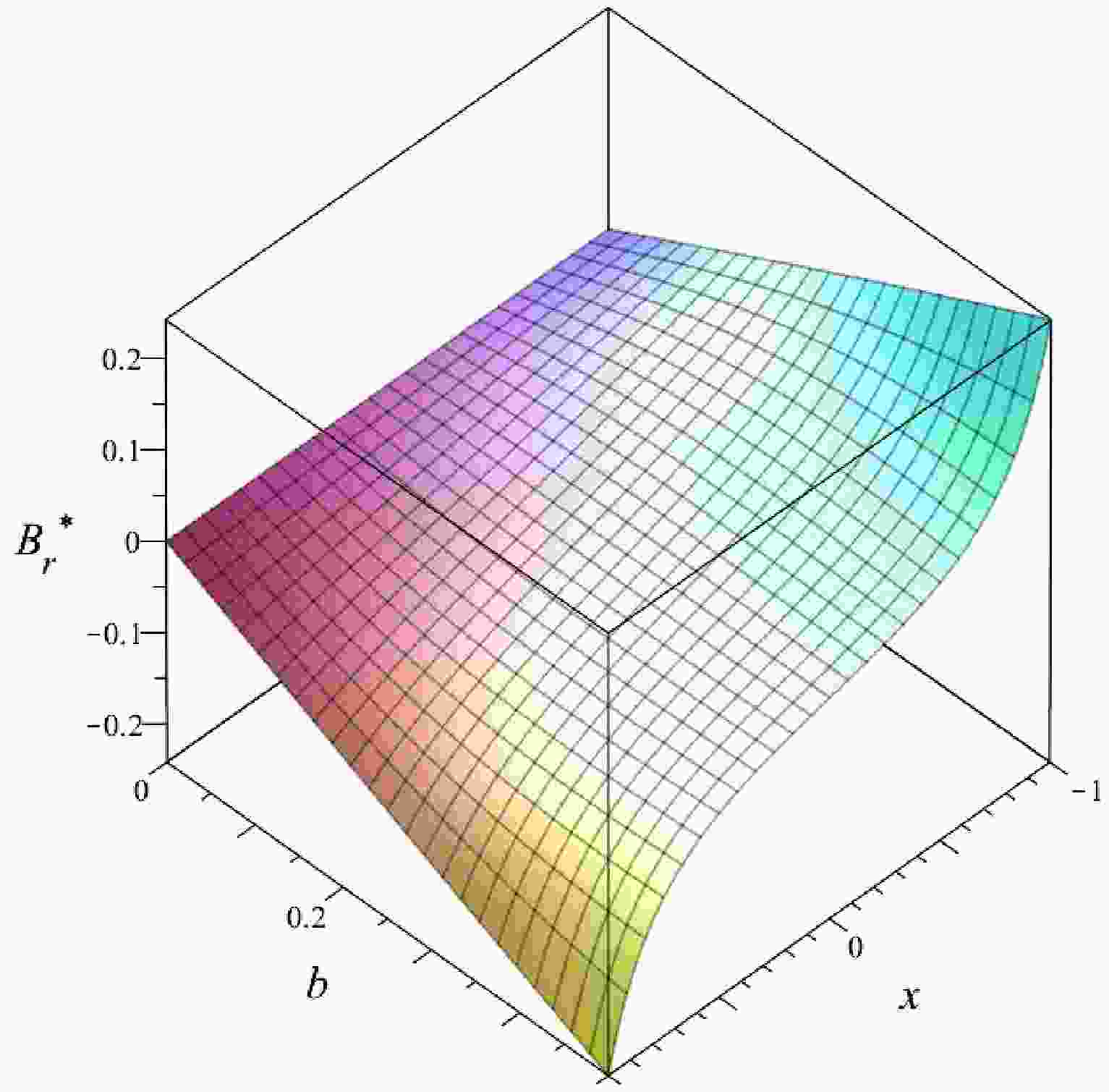
(13) The distinction becomes clear when considering that the Ernst magnetization process transforms the original line element into a new form, whereas the electric-magnetic duality transformation does not alter the underlying spacetime metric. This highlights the fundamental difference between the two approaches. Illustrations of magnetic fields near the black hole are given in Figs. 1, 2, 3, and 4. From these figures, one can learn how the magnetic field, described by Eqs. (77) and (78), changes from the south to the north pole at a fixed radius
$ r=2m $ and electric charge$ Q=0.1\; m $ , in the absence and presence of magnetic monopole P. In the following figures,$ B_r^* = B_r m^3 $ and$ B_x^* = B_x m^2 $ , representing the dimensionless magnetic field vector components. Hence, it becomes possible to discern the respective contributions of the external magnetic field and magnetic monopole parameters to the observed magnetic field surrounding the black hole. In this sense, one can also distinguish aspects of MdRN spacetime from the magnetized Reissner-Nordstrom black hole, as discussed in [16].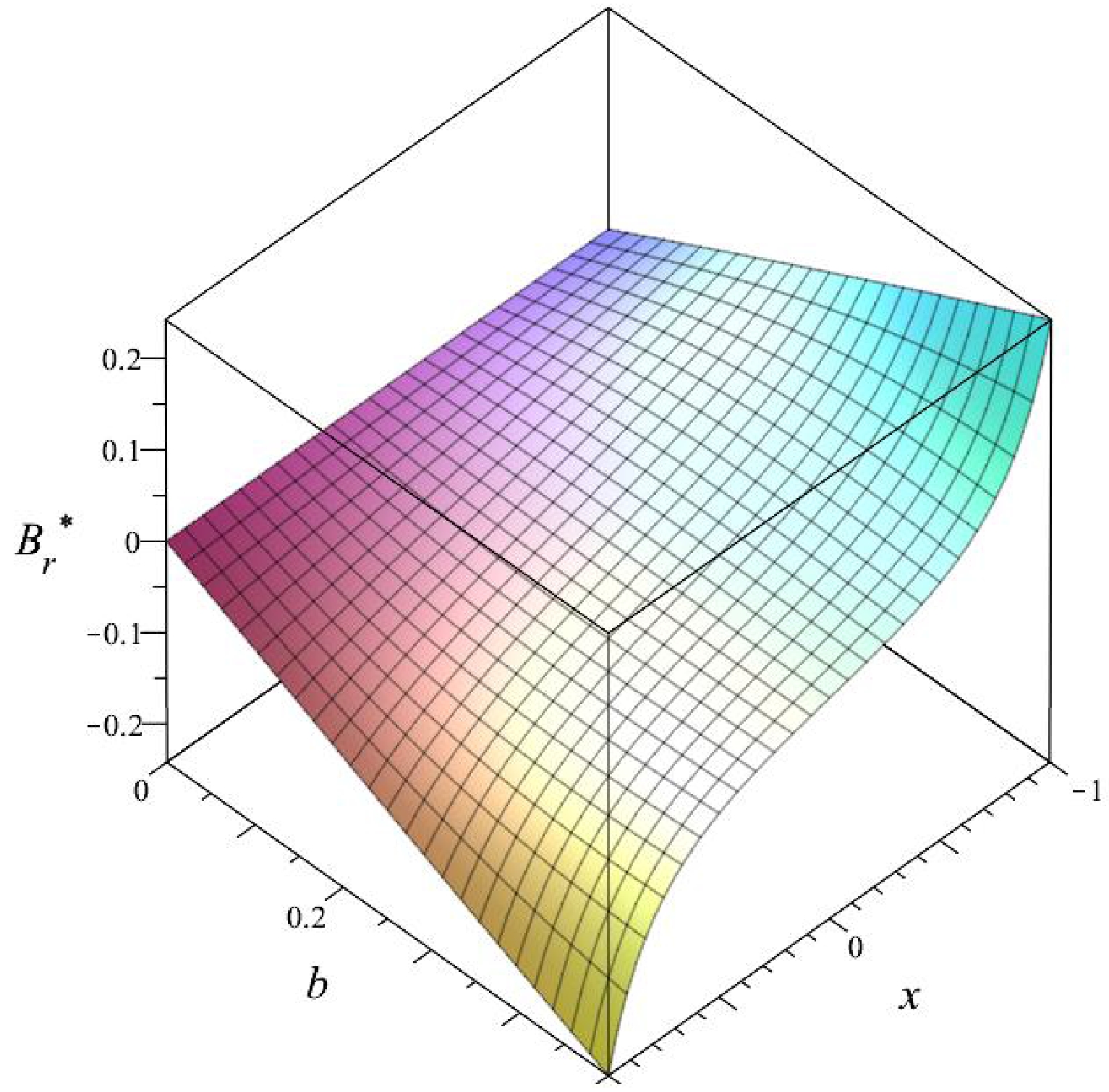
Figure 1. (color online) Numerical evaluation of Eq. (77) in the absence of magnetic monopole.
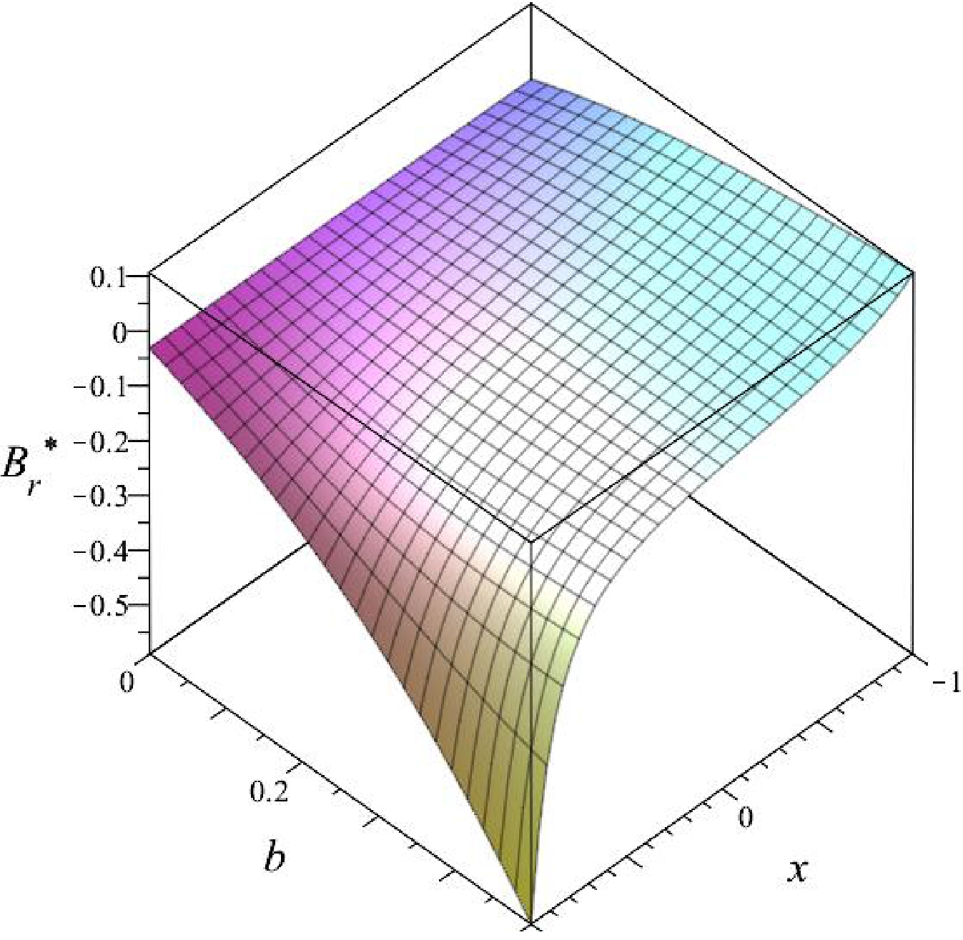
Figure 2. (color online) Numerical evaluation of Eq. (77) with
$ P=0.5\; m $ .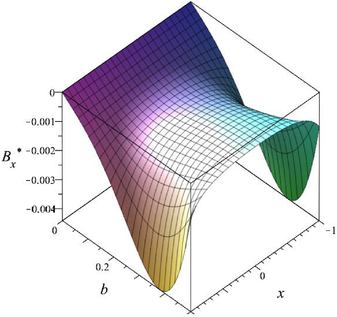
Figure 3. (color online) Numerical evaluation of Eq. (78) in the absence of magnetic monopole.

Figure 4. (color online) Numerical evaluation of Eq. (78) with
$ P=0.5\; m $ .The expressions determine the outer and inner horizons of the MdRN black hole
$ r_ \pm = m \pm \sqrt {m^2 - Q^2 - P^2 } \,. $

(14) These horizons coincide with those of the non-magnetized counterpart. The spacetime possesses both stationary and axial symmetries, which are characterized by the corresponding Killing vector
$ l^\mu \partial_\mu = \partial_t - \Omega_H \partial_\phi , $

(15) where
$ \Omega_H = \omega'(r=r_+) $ . The area of black hole can be computed using the formula$ A_H = \int\limits_{x = 1}^{ - 1} {\int\limits_{\phi = 0}^{2\pi } {\sqrt {g_{\phi \phi } g_{xx} } {\rm d}x{\rm d}\phi } } = 4\pi r_+^2 $

(16) and the corresponding entropy is
$ S_{BH} = A_H/4 $ . Furthermore, the Hawking temperature of the MdRN black hole can be expressed as$ T_H = \frac{\sqrt{m^2-Q^2-P^2}}{2\pi r_+^2}\,. $

(17) Notably, the area and Hawking temperature of the MdRN black hole remain the same as those of the non-magnetized version. However, the presence of an external magnetic field deforms the shape of the horizon, increasing its prolateness as the external magnetic field strength increases. It is also worth mentioning that the external magnetic field discussed here exists even in the absence of a magnetic charge for the black hole. The extreme case is characterized by
$ m^2 = P^2 + Q^2 $ , and at this state, the corresponding Hawking temperature becomes zero.However, it has been demonstrated that particle pairs can still be produced even in the extremal state of the black hole. This phenomenon can be interpreted as the Schwinger effect occurring near black holes, analogous to a similar effect observed in Minkowski space when subjected to a strong electromagnetic field. The Schwinger effect for Reissner-Nordstrom black holes was first introduced in [4], and its generalizations have been explored in various background scenarios [5−7]. In the context of the Kerr/CFT correspondence [21], a dual description of this effect can be formulated as well [4].
-
To obtain the near horizon geometry of the near extremal MdRN black hole, we employ the following coordinate transformation:
$ r \to r_0 + \varepsilon \rho \; \; ,\; \; t \to \frac{\tau }{\varepsilon }\; \; ,\; \; \phi \to \varphi + \varpi \frac{{{\rm d}\tau }}{\varepsilon } $

(18) together with the mass and charges relation
$ m \to r_0 + \frac{{\varepsilon ^2 D^2 }}{{2r_0 }} $

(19) where
$ r_0 = \sqrt{Q^2+P^2} $ and$ \varpi = -\frac{4bQ\left(1 \mp bP\right)}{r_0^2}\left(b^2 r_0^2 \mp 2 Pb + P^2 b^2 + 1 \right)\,. $

(20) The resulting metric due to this transformation is
$ \begin{aligned}[b] {\rm d}s^2 =\;& \Gamma \left( x \right)\left\{ { - \frac{{\left( {\rho ^2 - D^2 } \right){\rm d}\tau ^2 }}{{r_0^2 }} + \frac{{r_0^2 {\rm d}\rho ^2 }}{{\left( {\rho ^2 - D^2 } \right)}} + \frac{{r_0^2 {\rm d}\rho ^2 }}{{\Delta _x }}} \right\} \\&+ \frac{{r_0^2 \Delta _x }}{{\Gamma \left( x \right)}}\left( {{\rm d}\varphi + \kappa \rho {\rm d}\tau } \right)^2 \,, \end{aligned} $

(21) where
$ \begin{aligned}[b] \Gamma(x) =\;& 4b^2 r_0^2 \left(1\mp Pb\right)^2 x^2 - 4Pb \left(1 \mp Pb\right)\\&\times \left(1+ 2 P^2 b^2 + Q^2 b^2 \mp 2 Pb\right)x \\&+ \left(1+ 2 P^2 b^2 + Q^2 b^2 \mp 2 Pb\right)^2\,, \end{aligned} $

(22) and
$ \kappa = -\frac{4bQ\left(1 \mp Pb\right)\left(1+ 2 P^2 b^2 + Q^2 b^2 \mp 2 Pb\right)}{r_0^2}\,. $

(23) The near-horizon metric presented above exhibits a warped AdS
$ _3 $ geometry, which differs from the$\rm AdS_2 \times S^2 $ geometry associated with the near-horizon region of the Reissner-Nordstrom black hole. The emergence of this warped AdS$ _3 $ geometry can be attributed to the "dragging" effect induced by the presence of an external magnetic field surrounding the black hole. Notably, the presence of the warped AdS$ _3 $ factor is not exclusive to the near-horizon region of the MdRN black hole. It also arises in the near-horizon geometry of the Kerr-Newman black hole [5], exhibiting a similar warped AdS$ _3 $ structure.The associated gauge field to the near-horizon metric above in solving the Einstein-Maxwell equation reads
$ A_\mu dx^\mu = \frac{1}{{\Gamma \left( x \right)}}\left( {F_1 \left( x \right)rd\tau + F_2 \left( x \right){\rm d}\varphi } \right)\,, $

(24) where
$ \begin{aligned}[b]F_1(x) =\;& -Q \left(1 - Q^2 b^2 \mp 2 Pb\right) \Big[ b^4P^4 \mp 4 b^3 P^3 \\&\mp 2{P}^{2}{b}^{2} ( 2{b}^{2}{P}^{2}{x}^{2}+2{b}^{2}{Q}^{2}{x}^{2}-{P}^{2}{b}^{2}-{b}^{2}{Q}^{2}-3 ) \\& \pm 4Pb ( 2{b}^{2}{P}^{2}{x}^{2}+2{b}^{2}{Q}^{2}{x}^{2}-{P}^{2}{b}^{2}-\\&{b}^{2}{Q}^{2}-1 ) {P}^{4}{b}^{4}+2{P}^{2}{Q}^{2}{b}^{4}+{b}^{4}{Q}^{4}\\& -4{b}^{2}{P}^{2}{x}^{2} -4{b}^{2}{Q}^{2}{x}^{2}+2{P}^{2}{b}^{2}+2{b}^{2}{Q}^{2}+1 \Big]\,, \end{aligned} $

(25) and
$ \begin{aligned}[b] F_2 (x) =\;& P^4 b^3 \pm {P}^{3}{b}^{2} \left( 4bPx-3 \right) + b{P}^{2} ( 4{b}^{2}{P}^{2}{x}^{2}\\&+4{b}^{2}{Q}^{2}{x}^{2}+2{P}^{2}{b}^{2}+2{b}^{2}{Q}^{2}-9bPx+3 ) \\& \pm P ( 4{P}^{3}{b}^{3}x+4P{Q}^{2}{b}^{3}x-6{b}^{2}{P}^{2}{x}^{2}-6{b}^{2}{Q}^{2}{x}^{2}\\&-3{P}^{2}{b}^{2}-3{b}^{2}{Q}^{2}+6bPx -1 ) +{b}^{3}{P}^{4} \\& +2{b}^{3}{P}^{2}{Q}^{2}+{b}^{3}{Q}^{4}-3{P}^{3}x{b}^ {2}-3Px{b}^{2}{Q}^{2}\\&+2b{P}^{2}{x}^{2}+2b{Q}^{2}{x}^{2}+b{P}^{2} +b{Q}^{2}-Px \,. \end{aligned} $

(26) When considering the presence of a string-like singularity, the modified metric functions in the near-horizon metric presented above can be expressed as follows:
$ \begin{array}{*{20}{l}} \Gamma (x) \to {\tilde \Gamma} (x) = 4b^2 r_0^2 x^2 - 4bP (1+b^2 r_0^2) x + (1+ b^2 r_0^2)^2 \,, \end{array} $

(27) and
$ \kappa \to {\tilde \kappa} = -\frac{4 bQ (1+ b^2 r_0^2)}{r_0^2} \,. $

(28) Correspondingly, the functions in the near-horizon vector field are adjusted to
$ \begin{array}{*{20}{l}} F_1 (x) \to {\tilde F}_1 (x) = Q \left(b^2 r_0^2 -1 \right) \left((1+ b^2 r_0^2)^2 - 4 b^2 r_0^2\right)\,, \end{array} $

(29) and
$ \begin{array}{*{20}{l}} F_2 (x) \to {\tilde F}_2 (x) = 2b r_0^2 x^2 -P \left( 1 + 3\,{b}^{2} r_0^2 \right) x + b r_0^2 \left( 1 + {b}^{2} r_0^2 \right) \,. \end{array} $

(30) The Schwinger effect involving a pair of scalars carrying electric and magnetic monopoles has been extensively studied in [18]. In this discussion, we will specifically examine the interaction between the magnetic field of the magnetized dyonic black hole and a scalar particle possessing magnetic charge g. Sometimes, the scalar particle possessing magnetic charge is referred to as a "scalar dyon." The corresponding Klein-Gordon equation governing this interaction is given by
$ \begin{array}{*{20}{l}} \left( {\nabla _\mu - {\rm i}gB_\mu } \right)\left( {\nabla ^\mu - {\rm i}gB^\mu } \right)\Phi - \mu ^2 \Phi = 0\,. \end{array} $

(31) Note that
$ B_\mu $ is the dual vector field, which also plays an important role in the Ernst magnetization, as reviewed in appendix B. Since the black hole is purely magnetic, i.e.$ Q=0 $ , we can consider the ansatz$ \begin{array}{*{20}{l}} \Phi\left(\tau,\rho,x,\varphi\right) = {\rm e}^{-{\rm i}\omega \tau + i n \varphi} R(\rho) X(x)\,. \end{array} $

(32) Using this ansatz, the radial and angular parts of the Klein-Gordon can be read as
$ \partial _\rho \left( {D_\rho \partial _\rho R\left( \rho \right)} \right) + \left\{ {\frac{{P^2 \left( {g\rho c_k + P\omega } \right)^2 }}{{D_\rho }} - P^2 d_k^2 \mu ^2 - \lambda } \right\}R\left( \rho \right) = 0\,, $

(33) and
$ \partial _x \left( {\Delta _x \partial _x X\left( x \right)} \right) - \left\{ {\frac{{n^2 e_k^4 }}{{\Delta _x }} - 4P^3 bx\mu ^2 f_k - \lambda } \right\}R\left( \rho \right) = 0 \,, $

(34) respectively. In the given equations, the functions
$ c_k $ ,$ d_k $ ,$ e_k $ , and$ f_k $ are given by$ \begin{array}{*{20}{l}} c_{\pm} = 1 \mp 2Pb\; \; ,\; \; c_0 = 1-P^2 b^2\,, \end{array} $

(35) $ \begin{array}{*{20}{l}} d_{\pm} = 1 \mp 2 Pb + 2 P^2 b^2\; \; ,\; \; d_0 = 1+ P^2 b^2\,, \end{array} $

(36) $ \begin{array}{*{20}{l}} e_\pm = \left[1+ 2 Pb \left(1 \pm x\right)\left(1 \mp Pb\right)\right]\; \; ,\; \; e_0 = 1-2Pbx + P^2 b^2\,, \end{array} $

(37) and
$ \begin{array}{*{20}{l}} f_\pm = \left[1+ 2 Pb \left(1 \pm 2x\right)\left(1 \mp Pb\right)\right]\; \; ,\; \; f_0 = 1- Pbx + P^2 b^2\,. \end{array} $

(38) The subscript "k" denoting the specific case under consideration. Specifically,
$ k=+ $ corresponds to the upper hemisphere,$ k=- $ pertains to the lower hemisphere, in the spacetime with no string-like singularity. The$ k=0 $ indicates the case involving the existence of a string-like singularity.The radial Eq. (33) can be interpreted as describing a probe of a magnetic monopole, where the radial wave function is represented by
$ R(\rho) $ and it possesses an effective mass$ \mu_{{\rm eff},k}^2 = \mu^2 - \frac{c_k^2 g^2}{d_k^2} + \frac{\lambda}{P^2 d_k^2}\,, $

(39) moving in an AdS
$ _2 $ geometry with the radius$ L_k = P d_k $ . It is well-established that instability arises when the square of the effective mass violates the Breitenlohner-Freedman bound$ \mu _{{\rm{eff},k}}^{\rm{2}} \ge -\frac{1}{4 L_k^2}\,. $

(40) This violation is then interpreted as enabling the pair production near the horizon, taking the form of either Hawking radiation or the Schwinger effect.
To discuss the violation of the BF bound further, we introduce the quantity
$ \Theta = \mu_{{\rm eff},k}^2 + \frac{1}{4 L_k^2} \,. $

(41) A negative value of Θ indicates a violation of the BF bound, which leads to the pair production of scalar dyons. This scenario is possible when the charge-to-mass ratio of the dyonic scalar exceeds unity, as permitted by the Dirac quantization condition for the magnetic charge [10, 11]
$ \begin{array}{*{20}{l}} g q = 2n\,, \end{array} $

(42) where q is the electric charge and n is a positive even number. This phenomenon is reminiscent of the unstable tachyon mode in electrically charged scalars, which allows for the Schwinger effect near extremal Reissner-Nordstrom black holes [4]. In such cases, the mass of the created particle must be smaller than its charge. Numerical illustrations can be found in Figs. 5 and 6. These plots demonstrate that within the plausible range of astrophysical strong external magnetic fields [22], violations of the Breitenlohner-Freedman bound can occur.

Figure 5. (color online) Illustration for the violation of the BF bound for scalar dyons in the region of MdRN black hole in the absence of string-like singularity. Here,
$ \Theta = \mu_{{\rm eff},k}^2 + L_k^{-2}/4 $ . These plots are produced by taking$ \mu = 10^{-5} $ ,$ g=10^{-3} $ , and$ l=0 $ . Black curves are for the case$ P/m = 100 $ , whereas the blue ones represent$ P/m = 200 $ . Solid curves for the case$ k=+ $ and the dashed ones for$ k=- $ .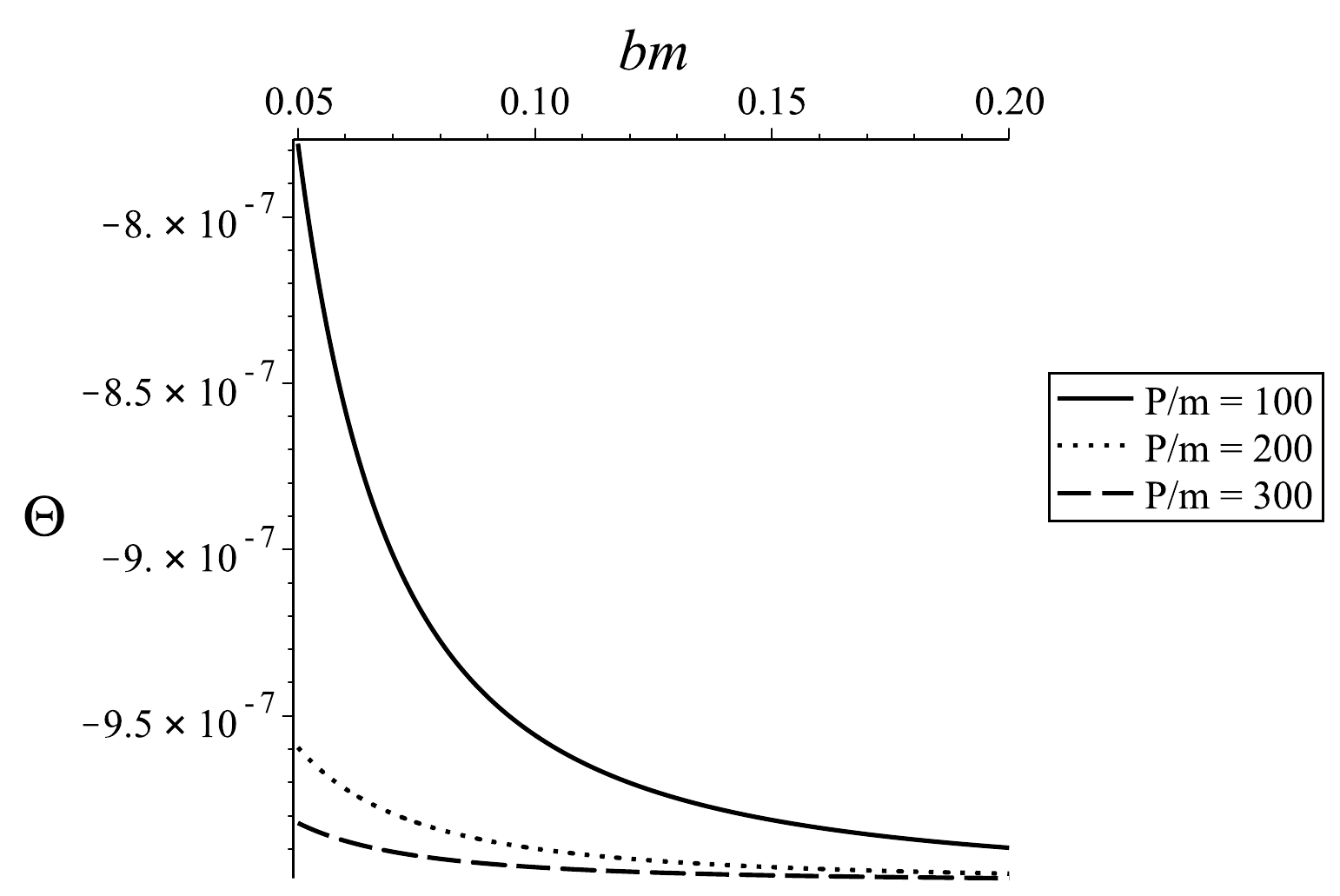
Figure 6. Illustration for the violation of the BF bound for scalar dyons in the region of the MdRN black hole with string-like singularity. Here,
$ \Theta = \mu_{{\rm eff},k}^2 + L_k^{-2}/4 $ . These plots are produced by taking$ \mu = 10^{-5} $ ,$ g=10^{-3} $ , and$ l=0 $ .In practical astrophysical situations, an exceptionally strong external magnetic field may arise near a black hole, such as the one generated by currents in an accretion disk, resulting in an unbounded strength of the magnetic field [23]. Therefore, if we assume the existence of such a field near a black hole, the violation of the BF bound is improbable for configurations without a string-like singularity. This is because as b approaches infinity, Θ approaches
$ \mu^2 $ . However, when the singularity is present, Θ approaches$ \mu^2 - g^2 $ as b tends to infinity, indicating the potential for a violation of the BF bound in environments with extremely strong external magnetic fields. -
The flux of a charged probe scalar field, governed by the Klein-Gordon Eq. (31), can be written as
$ {\cal W} = {\rm i} \int {{\rm d}x{\rm d}\phi } \sqrt {\left| g \right|} g^{\rho \rho } \left( {\Phi \tilde \nabla _\rho \Phi ^* - \Phi ^* \tilde \nabla _\rho \Phi } \right)\,, $

(43) where
$\tilde \nabla _\mu = \nabla_\mu - {\rm i} g {B}_\mu$ . In the specific case of the previously discussed near-horizon system, the flux can be expressed as$ \begin{array}{*{20}{l}} {\cal W} = {\rm i} \Xi \tilde \nabla _\rho \left(R \partial_\rho R^* - R^* \partial_\rho R\right), \end{array} $

(44) where
$\Xi = 2\pi \int {\rm d}x X^* X$ . Two different types of boundary conditions have been considered to analyze the absorption process related to scalar production. However, it has been demonstrated that these boundary conditions are equivalent [4]. Therefore, we will concentrate on one of them - the outer boundary condition. In this condition, we assume that the incoming flux vanishes at the outer boundary in the asymptotic region.This leads to a requirement imposed by flux conservation, which is expressed as follows:
$ \begin{array}{*{20}{l}} \left| {\cal W}_{\rm incident} \right| = \left| {\cal W}_{\rm reflected} \right| + \left| {\cal W}_{\rm transmitted} \right|\,, \end{array} $

(45) which leads to the Bogoliubov relation
$ \begin{array}{*{20}{l}} \left| \alpha \right|^2 = 1 + \left| \beta \right|^2\,. \end{array} $

(46) Above, α and β are the incorporated Bogoliubov coefficients. These coefficients can be expressed in terms of fluxes as follows [4]:
$ \left| \alpha \right|^2 = \frac{ {\cal W}_{\rm incident}}{ {\cal W}_{\rm reflected}}\,, $

(47) and
$ \left| \beta \right|^2 = \frac{ {\cal W}_{\rm transmitted}}{ {\cal W}_{\rm reflected}}\,. $

(48) It is recognized that
$ \left| \alpha \right|^2 $ represents the vacuum persistence amplitude, while$ \left| \beta \right|^2 $ corresponds to the mean number of produced pairs. Consequently, the absorption cross section can be expressed as$ \sigma_{\rm abs} = \frac{ {\cal W}_{\rm transmitted}}{ {\cal W}_{\rm incident}} = \frac{\left|\beta\right|^2}{\left|\alpha\right|^2}\,. $

(49) To determine the Bogoliubov coefficients associated with particle production near the horizon of the MdRN black hole, it is necessary to solve the radial Eq. (33). The solution to this equation can be expressed as
$ \begin{aligned}[b] R_k\left( \rho \right) =\;& C_1 F\Bigg( \frac{1}{2} + {\rm i}(p_k + n_k), \frac{1}{2} - {\rm i}p_k + {\rm i}n_k,1 \\&+ {\rm i}\left( {n_k + \nu} \right);\frac{1}{2} - \frac{\rho }{{2D}} \Bigg) \end{aligned} $

$ \begin{aligned}[b]&\times \left( {\rho + D} \right)^{\frac{{{\rm i}\left( {n_k - \nu} \right)}}{2}} \left( {\rho - D} \right)^{\frac{{{\rm i}\left( {n_k + \nu} \right)}}{2}} + C_2 F\Bigg( \frac{1}{2} + {\rm i}p_k\\& - {\rm i}\nu,\frac{1}{2} - {\rm i}(p_k + \nu),1 - {\rm i}\left( {n_k + \nu} \right);\frac{1}{2} - \frac{\rho }{{2D}} \Bigg) \\& \times \left( {\rho + D} \right)^{\frac{{{\rm i}\left( {n_k - \nu} \right)}}{2}} \left( {\rho - D} \right)^{ - \frac{{{\rm i}\left( {n_k + \nu} \right)}}{2}} \,, \end{aligned} $

(50) where
$ p_k = \left\{ { P^2 \left(g^2 c_k^2 - \mu^2 d_k^2 \right) -\left(l+\frac{1}{2}\right)^2} \right\}^{1/2} \,, $

(51) $ \begin{array}{*{20}{l}} n_k = g P c_k\,, \end{array} $

(52) $ \nu = \frac{{\omega P^2 }}{D}\,, $

(53) and
$ F\left(a,b,c;d\right) $ is a hypergeometric function. In the near-horizon region, the radial solution above can be approximated as$ \begin{aligned}[b]R_{H,k}\left( \rho \right) \approx\;& C_1 \left( {\rho + D} \right)^{\frac{{{\rm i}\left( {n_k - \nu} \right)}}{2}} \left( {\rho - D} \right)^{\frac{{{\rm i}\left( {n_k + \nu} \right)}}{2}} \\&+ C_2 \left( {\rho + D} \right)^{\frac{{{\rm i}\left( {n_k - \nu} \right)}}{2}} \left( {\rho - D} \right)^{ - \frac{{{\rm i}\left( {n_k + \nu} \right)}}{2}} \\ =\;& D^{\frac{{{\rm i}\left( {n_k - \nu} \right)}}{2}} \left( C_{H,k}^{\left( {{\rm{out}}} \right)} \left( {\rho - D} \right)^{\frac{{{\rm i}\left( {n_k + \nu} \right)}}{2}} + C_{H,k}^{\left( {{\rm{in}}} \right)} \left( {\rho - D} \right)^{ - \frac{{{\rm i}\left( {n_k + \nu} \right)}}{2}} \right) \,, \end{aligned} $

(54) where the identity
$ F\left(a,b,c;0\right)=1 $ has been used. Obviously, the coefficients$ C_{H,k}^{\left({{\rm{out}}} \right)} $ and$ C_{H,k}^{\left({{\rm{out}}} \right)} $ are$ C_1 $ and$ C_2 $ , respectively. At the boundary$ \rho \gg D $ , we can express the approximate radial solution as$ \begin{array}{*{20}{l}} R_{B,k} \left( \rho \right) \approx C_{B,k}^{\left( {\rm in} \right)} \rho^{ - {\rm i}p_k - { {1 \over 2}}} + C_{B,k}^{\left( {\rm out} \right)} \rho^{{\rm i}p_k - { {1 \over 2}}} \,, \end{array} $

(55) where the corresponding constants are
$ \begin{aligned}[b] {C_{B,k}^{\left( {\rm in} \right)}} =\;& {\Gamma \left( { - 2{\rm i}{p_k} } \right)}\left[{\frac{{\left( {2D} \right)^{{ {1 \over 2}} + {\rm i}\left( {n_k + {p_k} } \right)} \Gamma \left( {1 + {\rm i}\left( {n_k + {\nu} } \right)} \right)C_1}}{{2\Gamma \left( {{ {1 \over 2}} + {\rm i}\left( {n_k - {p_k} } \right)} \right)\Gamma \left( {{ {1 \over 2}} + {\rm i}\left( { {\nu} - {p_k} } \right)} \right)}}}\right.\\&\left. + {\frac{{\left( {2D} \right)^{{ {1 \over 2}} - {\rm i}\left( { {\nu} - {p_k} } \right)} \Gamma \left( {1 - {\rm i}\left( {n_k + {\nu} } \right)} \right)C_2}}{{2\Gamma \left( {{ {1 \over 2}} - {\rm i}\left( {n_k + {p_k} } \right)} \right)\Gamma \left( {{ {1 \over 2}} - {\rm i}\left( { {\nu} + {p_k} } \right)} \right)}}}\right]\,, \end{aligned} $

(56) and
$ \begin{aligned}[b] {C_{B,k} ^{\left( {\rm out} \right)}} =\;& {\Gamma \left( {2{\rm i}{p_k} } \right)} \left[{\frac{{\left( {2D} \right)^{{ {1 \over 2}} + {\rm i}\left( {n_k - {p_k} } \right)} \Gamma \left( {1 + {\rm i}\left( {n_k + {\nu} } \right)} \right)C_1}}{{2\Gamma \left( {{ {1 \over 2}} + {\rm i}\left( {n_k + {p_k} } \right)} \right)\Gamma \left( {{ {1 \over 2}} + {\rm i}\left( { {\nu} + {p_k} } \right)} \right)}}}\right. \\&\left. + {\frac{{\left( {2D} \right)^{{ {1 \over 2}} - {\rm i}\left( { {\nu} + {p_k} } \right)} \Gamma \left( {1 - {\rm i}\left( {n_k + {\nu} } \right)} \right)C_2}}{{2\Gamma \left( {{ {1 \over 2}} - {\rm i}\left( {n_k - {p_k} } \right)} \right)\Gamma \left( {{ {1 \over 2}} - {\rm i}\left( { {\nu} - {p_k} } \right)} \right)}}} \right]\,. \end{aligned} $

(57) Furthermore, by utilizing formula (44), we can calculate the following fluxes as
$ \begin{array}{*{20}{l}} {\cal W}_{H,k}^{\left({\rm in}\right)} = -2D \Xi \left| C_2 \right|^2 \left(n_k+s\right)\,, \end{array} $

(58) $ \begin{array}{*{20}{l}} {\cal W}_{H,k}^{\left({\rm out}\right)} = 2D \Xi \left| C_1 \right|^2 \left(n_k+s\right)\,, \end{array} $

(59) $ \begin{array}{*{20}{l}} {\cal W}_{B,k}^{\left({\rm in}\right)} = -2 \Xi \left| C_{B,k}^{\left({\rm in}\right)} \right|^2\,, \end{array} $

(60) and
$ \begin{array}{*{20}{l}} {\cal W}_{B,k}^{\left({\rm out}\right)} = 2 \Xi \left| C_{B,k}^{\left({\rm out}\right)} \right|^2\,. \end{array} $

(61) Obtaining the explicit Bogoliubov coefficients requires applying the boundary condition to the fluxes mentioned above. In this case, we adopt the outer boundary condition by setting
$ {\cal W}_{B,k}^{\left({\rm in}\right)} = 0 $ , which corresponds to zero incoming flux at the outer boundary. With this condition, we find the following expressions for the Bogoliubov coefficients$\begin{aligned}[b] {C_1} =\;& - {C_2}{\left( {2D} \right)^{\tfrac{1}{2} - {\rm i}\left( { \nu + n_k} \right)}}\\&\times\frac{{\Gamma \left( {1 - {\rm i}\left( {n_k + s_k } \right)} \right)\Gamma \left( {{ {1 \over 2}} + {\rm i}\left( {n_k - p_k } \right)} \right)\Gamma \left( {{ {1 \over 2}} + {\rm i}\left( { \nu - p_k } \right)} \right)}}{{\Gamma \left( {1 + {\rm i}\left( {n_k + \nu } \right)} \right)\Gamma \left( {{ {1 \over 2}} - {\rm i}\left( {n_k + p_k } \right)} \right)\Gamma \left( {{ {1 \over 2}} - {\rm i}\left( { \nu + p_k } \right)} \right)}}\,.\end{aligned} $

(62) Moreover, we can have
$ \begin{aligned}[b]& {\cal W}_{\rm incident} = {\cal W}_{H,k}^{\left({\rm out}\right)}\; \; ,\; \; {\cal W}_{\rm reflected} = {\cal W}_{H,k}^{\left({\rm in}\right)}\\& {\cal W}_{\rm transmitted} = {\cal W}_{B,k}^{\left({\rm out}\right)}\,, \end{aligned} $

(63) By applying the relation given in Eqs. (62) to equation (57), we can obtain the following expression
$ C_{B,k} ^{\left( {\rm out} \right)} = - \frac{{{C_2}{\left( {2D} \right)^{\tfrac{1}{2} - {\rm i}\left( { \nu + p_k } \right)}}}{\Gamma \left( {1 - {\rm i}\left( {n_k + \nu } \right)} \right)\Gamma \left( {2{\rm i}p_k } \right)\sinh \left( {2\pi p_k } \right)\sinh \left( {\pi \left( {n_k + \nu } \right)} \right)}}{{\Gamma \left( {{ {1 \over 2}} - {\rm i}\left( {n_k - p_k } \right)} \right)\Gamma \left( {{ {1 \over 2}} - {\rm i}\left( { \nu - p_k } \right)} \right)\cosh \left( {\pi \left( {n_k - p_k } \right)} \right)\cosh \left( {\pi \left( { \nu - p_k } \right)} \right)}}\,. $ 
(64) Now, by making use of the results in (47) and (48), the vacuum persistence amplitude and the mean number of produced pairs for the MdRN black hole can be expressed as
$ \begin{aligned}[b] \left| \alpha_k \right|^2 = \;&\frac{{{\cal W} _{\rm incident} }}{{{\cal W} _{\rm reflected} }} = \frac{{{\cal W} _{H,k} ^{\left( {\rm out} \right)} }}{{{\cal W} _{H,k}^{\left( {\rm in} \right)} }} \\=\;& \frac{{\cosh \left( {\pi \left( {n_k + {p_k} } \right)} \right)\cosh \left( {\pi \left( { {\nu} + {p_k} } \right)} \right)}}{{\cosh \left( {\pi \left( {n_k - {p_k} } \right)} \right)\cosh \left( {\pi \left( { {\nu} - {p_k} } \right)} \right)}}\,,\end{aligned} $

(65) $ \begin{aligned}[b] \left| \beta_k \right|^2 =\;& \frac{{{\cal W} _{\rm transmitted} }}{{{\cal W} _{\rm reflected} }} = \frac{{{\cal W} _{B,k} ^{\left( {\rm out} \right)} }}{{{\cal W} _{H,k}^{\left( {\rm in} \right)} }} \\=\;& \frac{{\sinh \left( {2\pi {p_k} } \right)\sinh \left( {\pi \left( {n_k + \nu } \right)} \right)}}{{\cosh \left( {\pi \left( {n_k - {p_k} } \right)} \right)\cosh \left( {\pi \left( { \nu - {p_k} } \right)} \right)}}\,, \end{aligned} $

(66) respectively, and the associated absorption cross section takes the form
$ {\sigma _{abs,k}} = \frac{{{\cal W} _{\rm transmitted} }}{{{\cal W} _{\rm incident} }} =\frac{{\sinh \left( {2\pi {p_k} } \right)\sinh \left( {\pi \left( {n_k + \nu } \right)} \right)}}{{\cosh \left( {\pi \left( {n_k + {p_k} } \right)} \right)\cosh \left( {\pi \left( { \nu + {_k} } \right)} \right)}}\,. $

(67) The expressions (65)−(67) above include contributions from both Hawking radiation and the Schwinger effect. However, pair production only occurs through the Schwinger effect in the extremal state. This state is obtained by taking
$ D\to 0 $ , which leads to$ \nu\to \infty $ . Consequently, the vacuum persistence amplitude and mean number of produced particles can be written as follows:$ \begin{aligned}[b] \left| \alpha_k \right|^2 =\;& \frac{{\cosh \left( {\pi \left( {n_k + p_k } \right)} \right)}}{{\cosh \left( {\pi \left( {n_k - p_k } \right)} \right)}}\exp \left( {2\pi p_k } \right)\; \; ,\\ \left| \beta_k \right|^2 =\;& \frac{{\sinh \left( {2\pi p_k } \right)}}{{\cosh \left( {\pi \left( {n_k - p_k } \right)} \right)}}\exp \left( \pi\left({n_k + p_k }\right) \right) \,, \end{aligned} $

(68) which corresponds to the absorption cross section
$ \sigma _{abs,k} = \frac{{\sinh \left( {2\pi p_k } \right)}}{{\cosh \left( {\pi \left( {n_k + p_k } \right)} \right)}}\exp \left( \pi\left({n_k - p_k }\right) \right)\,. $

(69) Here, one can observe a relation between the mean number of produced particles and the absorption cross section, namely
$ \begin{array}{*{20}{l}} \sigma _{abs,k} = - \left| \beta_k \right|^2 \left(p_k \to -p_k \right)\,. \end{array} $

(70) To verify the occurrence of particle production through the Schwinger effect, we present a numerical evaluation of
$ \sigma_{\text{abs},k} $ in Fig. 7. The plots in this figure demonstrate non-zero cross sections, indicating the presence of produced particles. This, in turn, corresponds to a non-zero mean number of produced particles. In all cases of interest, we find that a threshold for the external magnetic field allows the absorption cross section to exist. Within the range of possible astrophysical external magnetic field strengths [22], we observe that the cross section increases as the magnetic field strength grows.
Figure 7. Illustration of the absorption cross section for the scalar dyons near MdRN black hole. We consider
$ \mu = 10^{-5} $ ,$ g=10^{-3} $ ,$ l=0 $ , and$ P/m=100 $ . -
In this study, we investigated the phenomenon of pair production of magnetic monopoles as a Schwinger effect near a magnetized dyonic Reissner-Nordstrom black hole. We specifically focused on the magnetic interaction between the scalar dyon and the black hole. Our findings reveal that the Schwinger effect can indeed occur if the Dirac quantization condition is satisfied, allowing the charge-to-mass ratio of the dyon scalar to exceed unity. If no evidence of the Schwinger effect in the form of magnetic monopole pairs is observed, one may speculate that nature does not permit the existence of massive particles with large magnetic charges despite the suggestion by the Dirac quantization rule.
Our analysis of the Schwinger effect near the magnetized dyonic Reissner-Nordstrom black hole does not extend to the possible dual CFT description elaborated in [4, 5]. However, we believe that such an extension is straightforward by following the prescription outlined in [4, 5], as it heavily relies on the established dictionary of the Kerr/CFT correspondence [21, 24]. The compatibility between the Kerr/CFT correspondence and the pair production analysis near the (near)-extremal black hole horizon is evident, as it is related to the AdS
$ _2\times $ S$ ^2 $ or warped AdS$ _3 $ geometries that are present in the near horizon of the considered black hole. It is well-known that this AdS$ _2\times $ S$ ^2 $ or warped AdS$ _3 $ structure forms the foundation for constructing the Kerr/CFT correspondence.Including or avoiding string-like singularity in the analysis has led to notable distinctions in the properties associated with the Schwinger effect. This observation motivates the investigation of the role of the Misner string in NUT spacetime and its potential influence on pair production. Recently, the magnetized version of the Reissner-Nordstrom-Taub-NUT spacetime has been reported [20], opening up the possibility to explore the corresponding pair production in this spacetime. We consider this to be a problem in future research.
-
I express gratitude to the anonymous referees for their valuable comments.
-
In the absence of string-like singularity, the magnetized vector solution accompanying the spacetime metric (7) in solving the Einstein-Maxwell equations can be expressed as
$ \begin{aligned}[b]A_\mu dx^\mu = \;&\frac{{Q\left(a_0 \pm a_1 + a_2 \pm a_3 + a_4\right) }}{{r\left(b_0 \pm b_1 + b_2 \pm b_3 + b_4\right) }}{\rm d}t \\&+ \frac{{c_0 \pm c_1 + c_2 \pm c_3 + c_4 }}{{d_0 \pm d_1 + d_2 \pm d_3 + d_4 }}{\rm d}\phi \,, \end{aligned}\tag{A1} $

where
$ \begin{aligned}[b] a_0 =\;& {b}^{6}{P}^{6}{x}^{6}+3{b}^{6}{P}^{4}{x}^{6}{Q}^{2}-2{b}^{6}{x}^{6}mr{P}^{4}-{b}^{6}{P}^{4}{x}^{6}{r}^{2}+3{b}^{6}{P}^{2}{x}^{6}{Q}^{4}-4{b}^{6}{x}^{6}mr{P}^{2}{Q}^{2}-2{b}^{6}{r}^{2}{x}^{6}{P}^{2}{Q}^{2}\\& +4{b}^{6}{x}^{6}m{r}^{3}{P}^{2}-{b}^{6}{P}^{2}{x}^{6}{r}^{4}+{b}^{6}{x}^{6}{Q}^{6}-2{b}^{6}{x}^{6}mr{Q}^{4}-{b}^{6}{Q}^{4}{x}^{6}{r}^{2}+4{b}^{6}{x}^{6}m{r}^{3}{Q}^{2}-{b}^{6}{r}^{4}{x}^{6}{Q}^{2}-2{b}^{6}{x}^{6}m{r}^{5}\\& +{b}^{6}{r}^{6}{x}^{6}+3{b}^{6}{P}^{4}{x}^{4}{r}^{2}+6{b}^{6}{P}^{2}{x}^{4}{Q}^{2}{r}^{2}-4{b}^{6}{x}^{4}m{r}^{3}{P}^{2}-2{b}^{6}{P}^{2}{x}^{4}{r}^{4}+3{b}^{6}{Q}^{4}{x}^{4}{r}^{2}-4{b}^{6}{x}^{4}m{r}^{3}{Q}^{2}\\& -2{b}^{6}{x}^{4}{Q}^{2}{r}^{4}+4{b}^{6}{x}^{4}m{r}^{5}-{b}^{6}{r}^{6}{x}^{4}+3{b}^{6}{P}^{2}{x}^{2}{r}^{4}+3{b}^{6}{r}^{4}{x}^{2}{Q}^{2}-2{b}^{6}{x}^{2}m{r}^{5}-{b}^{6}{r}^{6}{x}^{2}-9{b}^{4}{P}^{4}{x}^{4} \\&-18{b}^{4}{P}^{2}{x}^{4}{Q}^{2}+12{b}^{4}{x}^{4}mr{P}^{2}+2{b}^{4}{r}^{2}{x}^{4}{P}^{2}-9{b}^{4}{Q}^{4}{x}^{4}+12{b}^{4}{x}^{4}mr{Q}^{2}+2{b}^{4}{r}^{2}{x}^{4}{Q}^{2}+{b}^{6}{r}^{6}-4{b}^{4}{x}^{4}m{r}^{3}\\&-{b}^{4}{r}^{4}{x}^{4}-14{b}^{4}{r}^{2}{P}^{2}{x}^{2}-14{b}^{4}{r}^{2}{Q}^{2}{x}^{2}+4{b}^{4}{x}^{2}m{r}^{3}+6{b}^{4}{r}^{4}{x}^{2}+16{b}^{3}{P}^{3}{x}^{3}+16{b}^{3}P{x}^{3}{Q}^{2} \\& -16{b}^{3}{x}^{3}mrP -5{b}^{4}{r} ^{4}+16{b}^{3}Px{r}^{2}-9{b}^{2}{P}^{2}{x}^{2}-9{b}^{2}{Q}^{2}{x}^{2}+6{b}^{2}{x}^{2}mr-{b}^{2}{r}^{2}{x}^{2}-5{b}^{2}{r}^{2}+1 \end{aligned} $ 
$ \begin{aligned}[b] a_1 =\;& 2Pb \left( 9{b}^{4}{P}^{4}{x}^{4}+18{b}^{4}{P}^{2}{x}^{4}{Q}^{2} -12{b}^{4}{x}^{4}mr{P}^{2}-2{b}^{4}{r}^{2}{x}^{4}{P}^{2}+9{b}^{4}{Q}^{4}{x}^{4}-12{b}^{4}{x}^{4}mr{Q}^{2} \right. \\&-2{b}^{4}{r}^{2}{x}^{4}{Q }^{2}+4{b}^{4}{x}^{4}m{r}^{3}+{b}^{4}{r}^{4}{x}^{4}+14{b}^{4}{r}^{2}{P}^{2}{x}^{2}+14{b}^{4}{r}^{2}{Q}^{2}{x}^{2}-4{b}^{4}{x}^{2}m{r}^{3}-6{b}^{4}{r}^{4}{x}^{2} \\&-24{b}^{3}{P}^{3}{x}^{3}-24{b}^{3}P{x}^{3}{Q}^{2}+24{b}^{3}{x}^{3}mrP+5{b}^{4}{r}^{4}-24{b}^{3}Px{r} ^{2}+18{b}^{2}{P}^{2}{x}^{2}+18{b}^{2}{Q}^{2}{x}^{2}\\& \left. -12{b}^{2}{x}^{2}mr+2{b}^{2}{r}^{2}{x}^{2}+10{b}^{2}{r}^{2}-3 \right) \end{aligned} $

$ \begin{aligned}[b] a_2 =\;& -{P}^{2}{b}^{2} \left( 9{b}^{4}{P}^{4}{x}^{4}+18{b}^{4}{P}^{2}{x}^ {4}{Q}^{2}-12{b}^{4}{x}^{4}mr{P}^{2}-2{b}^{4}{r}^{2}{x}^{4}{P}^{2}+9{b}^{4}{Q}^{4}{x}^{4}-12{b}^{4}{x}^{4}mr{Q}^{2} \right. \\& -2{b}^{4}{r}^{2}{x}^{4}{Q}^{2}+4{b}^{4}{x}^{4}m{r}^{3}+{b}^{4}{r}^{4}{x}^{4}+14{b}^{4}{r}^{2}{P}^{2}{x}^{2}+14{b}^{4}{r}^{2}{Q}^{2}{x}^{2}-4{b}^{4} {x}^{2}m{r}^{3}-6{b}^{4}{r}^{4}{x}^{2}\\& -48{b}^{3}{P}^{3}{x}^{3} -48{b}^{3}P{x}^{3}{Q}^{2}+48{b}^{3}{x}^{3}mrP+5{b}^{4}{r}^{4}-48{b}^{3}Px{r}^{2}+54{b}^{2}{P}^{2}{x}^{2}+54{b}^{2}{Q}^{2}{x}^{2}\\& \left. -36 {b}^{2}{x}^{2}mr+6{b}^{2}{r}^{2}{x}^{2}+30{b}^{2}{r}^{2}-15 \right) \end{aligned}$

$ \begin{aligned}[b] a_3 =\;& -4{P}^{3}{b}^{3} \left( 4{b}^{3}{P}^{3}{x}^{3}+4{b}^{3}P{x}^{3}{Q}^{2}-4{b}^{3}{x}^{3}mrP+4{b}^{3}Px{r}^{2}-9{b}^{2}{P}^{2}{x}^{2} \right. \\&\left. -9{b}^{2}{Q}^{2}{x}^{2}+6{b}^{2}{x}^{2}mr-{b}^{2}{r}^{2}{x}^{2}-5{b}^{2}{r}^{2}+5 \right) \end{aligned}$

$ a_4 = -{P}^{4}{b}^{4} \left( 9{b}^{2}{P}^{2}{x}^{2}+9{b}^{2}{Q}^{2}{x}^{2}-6{b}^{2}{x}^{2}mr+{b}^{2}{r}^{2}{x}^{2}+5{b}^{2}{r}^{2}-15 \right) $

$\begin{aligned}[b] b_0 =\;& {b}^{4}{P}^{4}{x}^{4}+2{b}^{4}{P}^{2}{x}^{4}{Q}^{2}-2{b}^{4}{r}^{2}{x}^{4}{P}^{2}+{b}^{4}{Q}^{4}{x}^{4}-2{b}^{4}{r}^{2}{x}^{4}{Q}^{2}+ {b}^{4}{r}^{4}{x}^{4}+2{b}^{4}{r}^{2}{P}^{2}{x}^{2}+2{b}^{4}{r}^{2}{Q}^{2}{x}^{2}-2{b}^{4}{r}^{4}{x}^{2} \\& -4{b}^{3}{P}^{3}{x}^{3}-4{b}^{3}P{x}^{3}{Q}^{2}+4{b}^{3}P{x}^{3}{r}^{2}+{b}^{4}{r}^{4}-4{b}^ {3}Px{r}^{2}+6{b}^{2}{P}^{2}{x}^{2}+6{b}^{2}{Q}^{2}{x}^{2}-2{b}^{2}{r}^{2}{x}^{2}+2{b}^{2}{r}^{2}-4bPx+1 \end{aligned}$

$ b_1 = 4Pb \left( {b}^{3}{P}^{3}{x}^{3}+{b}^{3}P{x}^{3}{Q}^{2}-{b}^{3}P{x}^ {3}{r}^{2}+{b}^{3}Px{r}^{2}-3{b}^{2}{P}^{2}{x}^{2}-3{b}^{2}{Q}^{2} {x}^{2}+{b}^{2}{r}^{2}{x}^{2}-{b}^{2}{r}^{2}+3bPx-1 \right) $

$ b_2 = 2{P}^{2}{b}^{2} \left( 3{b}^{2}{P}^{2}{x}^{2}+3{b}^{2}{Q}^{2}{x} ^{2}-{b}^{2}{r}^{2}{x}^{2}+{b}^{2}{r}^{2}-6bPx+3 \right) $

$ b_3 = 4{P}^{3}{b}^{3} \left( bPx-1 \right) $

$ b_4 = P^4 b^4 $

$\begin{aligned}[b] c_0 =\;& -{b}^{3}{P}^{4}{x}^{4}-2{b}^{3}{P}^{2}{x}^{4}{Q}^{2}+2{b}^{3}{r}^{2}{x}^{4}{P}^{2}-{b}^{3}{Q}^{4}{x}^{4}+2{b}^{3}{r}^{2}{x}^{4}{Q}^{2} -{b}^{3}{r}^{4}{x}^{4}-2{b}^{3}{r}^{2}{P}^{2}{x}^{2}-2{b}^{3}{r}^{2}{Q}^{2}{x}^{2}+2{b}^{3}{r}^{4}{x}^{2} \\& +3{P}^{3}{x}^{3}{b}^{2}+3 P{x}^{3}{b}^{2}{Q}^{2}-3P{x}^{3}{b}^{2}{r}^{2}-{b}^{3}{r}^{4}+3Px{b}^{2}{r}^{2}-3b{P}^{2}{x}^{2}-3b{Q}^{2}{x}^{2}+b{r}^{2}{x}^{2}-b{r}^{2}+Px \end{aligned}$

$ c_1 =-P \left( 4{b}^{3}{P}^{3}{x}^{3}+4{b}^{3}P{x}^{3}{Q}^{2}-4{b}^{3 }P{x}^{3}{r}^{2}+4{b}^{3}Px{r}^{2}-9{b}^{2}{P}^{2}{x}^{2} -9{b}^{2}{Q}^{2}{x}^{2}+3{b}^{2}{r}^{2}{x}^{2}-3{b}^{2}{r}^{2}+6bPx-1 \right) $

$ c_2 = -{P}^{2}b \left( 6{b}^{2}{P}^{2}{x}^{2}+6{b}^{2}{Q}^{2}{x}^{2}-2 {b}^{2}{r}^{2}{x}^{2}+2{b}^{2}{r}^{2}-9bPx+3 \right) $

$ c_3 = -{P}^{3}{b}^{2} \left( 4 bPx-3 \right) $

$ c_4 = - P^4 b^3 $

$ \begin{aligned}[b] d_0 =\;& {b}^{4}{P}^{4}{x}^{4}+2{b}^{4}{P}^{2}{x}^{4}{Q}^{2}-2{b}^{4}{r}^{2}{x}^{4}{P}^{2}+{b}^{4}{Q}^{4}{x}^{4}-2{b}^{4}{r}^{2}{x}^{4}{Q}^{2}+ {b}^{4}{r}^{4}{x}^{4}+2{b}^{4}{r}^{2}{P}^{2}{x}^{2}+2{b}^{4}{r}^{2}{Q}^{2}{x}^{2}-2{b}^{4}{r}^{4}{x}^{2} \\& -4{b}^{3}{P}^{3}{x}^{3} -4{b}^{3}P{x}^{3}{Q}^{2}+4{b}^{3}P{x}^{3}{r}^{2}+{b}^{4}{r}^{4}-4{b}^{3}Px{r}^{2}+6{b}^{2}{P}^{2}{x}^{2}+6{b}^{2}{Q}^{2}{x}^{2}-2{b}^{2}{r}^{2}{x}^{2}+2{b}^{2}{r}^{2}-4bPx+1 \end{aligned}$

$ d_1 = 4Pb \left( {b}^{3}{P}^{3}{x}^{3}+{b}^{3}P{x}^{3}{Q}^{2}-{b}^{3}P{x}^ {3}{r}^{2}+{b}^{3}Px{r}^{2}-3{b}^{2}{P}^{2}{x}^{2}-3{b}^{2}{Q}^{2} {x}^{2}+{b}^{2}{r}^{2}{x}^{2}-{b}^{2}{r}^{2}+3bPx-1 \right) $

$ d_2 = 2{P}^{2}{b}^{2} \left( 3{b}^{2}{P}^{2}{x}^{2}+3{b}^{2}{Q}^{2}{x} ^{2}-{b}^{2}{r}^{2}{x}^{2}+{b}^{2}{r}^{2}-6bPx+3 \right) $

$ d_3 = 4 {P}^{3}{b}^{3} \left( bPx-1 \right) $

$ d_4 = P^4 b^4 $

The accompanying vector solution in the presence of string-like singularity is
$ A_\mu dx^\mu = \frac{Q a_0}{rb_0} {\rm d}t + \frac{c_0}{d_0} {\rm d}\phi \,. \tag{A2} $

The electric and magnetic field measured by an observer with four-velocity
$ u^\mu $ are given by$ E_\alpha = - F_{\alpha \mu } u^\mu \,, \tag{A3} $

and
$ B_\alpha = \frac{1}{2}\epsilon _{\alpha \beta \mu \nu } F^{\beta \mu } u^\nu \,. \tag{A4} $

Accordingly, the associated radial component of electric and magnetic fields measured by a static observer
$ u^\mu = \left[1,0,0,0\right] $ are$ \begin{aligned}[b] E_r =\;& -\frac{Q}{r^2 {\cal X}^2} \left\{ \left( {P}^{2}{x}^{2}-{r}^{2}{x}^{2}+{Q}^{2}{x}^{2}-{r}^{2} \right) \left( {P}^{2}{x}^{2}-{r}^{2}{x}^{2}+{Q}^{2}{x}^{2}+{r}^{2} \right)^{4} b^{10} -4Px \left( {P}^{2}{x}^{2}-{r}^{2}{x}^{2} \right. \right. \\& \left. +{Q}^{2}{x}^{2}+{r}^{2} \right) ^{2} \left( {P}^{4}{x}^{4}+2{Q}^{2}{x}^{4}{P}^{2}-2{r}^{2 }{P}^{2}{x}^{2} -4{x}^{4}m{r}^{3}+3{r}^{4}{x}^{4}+{Q}^{4}{x}^{4}+4 {x}^{2}m{r}^{3}-2{r}^{2}{Q}^{2}{x}^{2}-3{r}^{4} \right) b^9\\& - \left( {P}^{2}{x}^{2}-{r}^{2}{x}^{2}+{Q}^{2}{x}^{2}+{r}^{2} \right) \left( 11{r}^{6}-17{r}^{6}{x}^{2}+{r}^{6}{x}^{4}+3{Q}^{6}{x}^{6 }+3{P}^{6}{x}^{6}+5{r}^{6}{x}^{6}-23{x}^{6}{P}^{2}{r}^{4}\right.\\& +49{r }^{2}{Q}^{4}{x}^{4}-34{r}^{4}{Q}^{2}{x}^{4} -23{r}^{4}{Q}^{2}{x}^{6 }+49{r}^{2}{P}^{4}{x}^{4}-49{r}^{2}{Q}^{4}{x}^{6} -49{r}^{2}{P}^{ 4}{x}^{6}-16{x}^{2}m{r}^{5}+32{x}^{4}m{r}^{5} \\& -16{x}^{6}m{r}^{5}+ 57{r}^{4}{Q}^{2}{x}^{2}-34{P}^{2}{r}^{4}{x}^{4}+57{P}^{2}{r}^{4} {x}^{2}+9{x}^{6}{P}^{4}{Q}^{2}+9{x}^{6}{P}^{2}{Q}^{4}+98{r}^{2}{ Q}^{2}{x}^{4}{P}^{2} \\&\left. -98{r}^{2}{Q}^{2}{x}^{6}{P}^{2}-80{x}^{4}m{r}^ {3}{Q}^{2}-80{x}^{4}m{r}^{3}{P}^{2}+80{x}^{6}m{r}^{3}{Q}^{2}+80{ x}^{6}m{r}^{3}{P}^{2} \right) b^8 + 8Px \left( 6{r}^{6}-9{r}^{6}{x}^{2} \right. \\&+6{Q}^{6}{x}^{6}+6{P}^{6} {x}^{6}+3{r}^{6}{x}^{6}+8{x}^{6}{P}^{2}{r}^{4}+18{r}^{2}{Q}^{4}{ x}^{4}-26{r}^{4}{Q}^{2}{x}^{4}+8{r}^{4}{Q}^{2}{x}^{6}+18{r}^{2}{ P}^{4}{x}^{4}-25{r}^{2}{Q}^{4}{x}^{6} \\&-25{r}^{2}{P}^{4}{x}^{6}-12 {x}^{2}m{r}^{5}+24{x}^{4}m{r}^{5}-12{x}^{6}m{r}^{5}+18{r}^{4}{Q} ^{2}{x}^{2}-26{P}^{2}{r}^{4}{x}^{4}+18{P}^{2}{r}^{4}{x}^{2}+18{x }^{6}{P}^{4}{Q}^{2}+18{x}^{6}{P}^{2}{Q}^{4} \\&\left. +36{r}^{2}{Q}^{2}{x}^{4 }{P}^{2} -50{r}^{2}{Q}^{2}{x}^{6}{P}^{2}-20{x}^{4}m{r}^{3}{Q}^{2}- 20{x}^{4}m{r}^{3}{P}^{2}+20{x}^{6}m{r}^{3}{Q}^{2}+20{x}^{6}m{r}^ {3}{P}^{2} \right) b^7 \\& + \left( 10{r}^{6}{x}^{2}-10{r}^{6}+10{r}^{6}{x}^{4}-62{Q}^{6}{x}^{6}- 126{P}^{6}{x}^{6}-10{r}^{6}{x}^{6}-26{x}^{6}{P}^{2}{r}^{4}-22{ r}^{2}{Q}^{4}{x}^{4}+28{r}^{4}{Q}^{2}{x}^{4} \right. \\&-26{r}^{4}{Q}^{2}{x}^{ 6}-150{r}^{2}{P}^{4}{x}^{4}+98{r}^{2}{Q}^{4}{x}^{6}+290{r}^{2}{P }^{4}{x}^{6}+32{x}^{2}m{r}^{5}-64{x}^{4}m{r}^{5}+32{x}^{6}m{r}^{ 5}-2{r}^{4}{Q}^{2}{x}^{2}+92{P}^{2}{r}^{4}{x}^{4} \\&-66{P}^{2}{r}^{ 4}{x}^{2}-314{x}^{6}{P}^{4}{Q}^{2}-250{x}^{6}{P}^{2}{Q}^{4}-172{ r}^{2}{Q}^{2}{x}^{4}{P}^{2}+388{r}^{2}{Q}^{2}{x}^{6}{P}^{2}+32{x}^ {4}m{r}^{3}{Q}^{2}+160{x}^{4}m{r}^{3}{P}^{2} \\&\left. -32{x}^{6}m{r}^{3}{Q}^ {2}-160{x}^{6}m{r}^{3}{P}^{2} \right) b^6 + 8Px \left( 10{x}^{4}m{r}^{3}+21{P}^{4}{x}^{4}-2{r}^{4}{x}^{4}- 25{r}^{2}{x}^{4}{P}^{2}-25{r}^{2}{x}^{4}{Q}^{2} \right. \\&\left. +21{Q}^{4}{x}^{4} +42{Q}^{2}{x}^{4}{P}^{2}+4{r}^{2}{P}^{2}{x}^{2} +3{r}^{4}{x}^{2}+ 4{r}^{2}{Q}^{2}{x}^{2}-10{x}^{2}m{r}^{3}-{r}^{4} \right) b^5 + \left( 52{r}^{2}{x}^{4}{Q}^{2}-4{r}^{2}{Q}^{2}{x}^{2} \right. \\&-62{Q}^{4}{x}^{4} +52{r}^{2}{x}^{4}{P}^{2}+10{r}^{4}{x}^{4}-188{Q}^{2}{x}^{4}{P}^{ 2}-126{P}^{4}{x}^{4}-20{r}^{4}{x}^{2}-16{x}^{4}m{r}^{3}+16{x}^ {2}m{r}^{3}+10{r}^{4} \\&\left. +60{r}^{2}{P}^{2}{x}^{2} \right) b^4 + 8xP \left( 6{Q}^{2}{x}^{2}+{r}^{2}{x}^{2}-6{r}^{2}+6{P}^{2}{x}^{2} \right) b^3 + \left( 11{r}^{2}-5{r}^{2}{x}^{2}-3{P}^{2}{x}^{2}-3{Q}^{2}{x}^{2} \right) b^2\left. - 4xPb +1 \right\} \,, \end{aligned}\tag{A5}$

$ \begin{aligned}[b] E_x =\;& \frac{2Qb}{r {\cal X}^2} \left\{ x \left( {P}^{2}{x}^{2}+{Q}^{2}{x}^{2}-{r}^{2}{x}^{2}+{r}^{2} \right)^{4} \Delta_r b^9 -2P \left( {P}^{2}{x}^{2}+{Q}^{2}{x}^{2}-{r}^{2}{x}^{2}+{r}^{2} \right) ^{2} \left( 3{P}^{4}{x}^{4} \right. \right. \\&-6{P}^{2}{x}^{4}mr+6{Q}^{2}{x}^{4}{P}^{2}+2{r}^{2}{P}^{2}{x}^{2}-6{x}^{4}mr{Q}^{2}+6{x}^{4}m {r}^{3}+3{Q}^{4}{x}^{4}-3{r}^{4}{x}^{4}+2{r}^{2}{Q}^{2}{x}^{2} \\& \left. -2 {x}^{2}m{r}^{3}-{r}^{4} \right) b^8 + 4x \left( {P}^{2}{x}^{2}+{Q}^{2}{x}^{2}-{r}^{2}{x}^{2}+{r}^{2} \right) \left( 3{P}^{4}{x}^{2}-4{r}^{2}{P}^{2}{x}^{2}+6{x}^{2} {Q}^{2}{P}^{2} \right. \\&\left. -{r}^{2}{P}^{2}-4{r}^{2}{Q}^{2}{x}^{2}+{r}^{4}{x}^{2}+ 3{x}^{2}{Q}^{4}-{r}^{4}-{r}^{2}{Q}^{2} \right) \left( {P}^{2}{x}^{2 }+{Q}^{2}{x}^{2}-2{x}^{2}mr+{r}^{2}{x}^{2}+{r}^{2} \right) b^7 \\&+ 4Pr{x}^{2} \left( 2{x}^{4}{P}^{2}{r}^{3} -3{x}^{4}{r}^{5}-6{r}^{5}{x}^{2}+9{r}^{5}+5 {r}^{4}{x}^{4}m+2{r}^{4}{x}^{2}m-7{r}^{4}m+2{x}^{4}{Q}^{2}{r}^ {3} \right. \\&+18{r}^{3}{P}^{2}{x}^{2}+18{r}^{3}{Q}^ {2}{x}^{2}-6{r}^{2}{x}^{4}m{P}^{2}-6{r}^{2}{x}^{4}m{Q}^{2}-14{r} ^{2}{x}^{2}m{P}^{2}-14{r}^{2}{x}^{2}m{Q}^{2} \\&\left. +r{P}^{4}{x}^{4}+r{Q}^{4 }{x}^{4}+2r{Q}^{2}{x}^{4}{P}^{2}+{x}^{4}{P}^{4}m+2{x}^{4}{P}^{2}m{Q}^{2}+{x}^{4}m{Q}^{4} \right) b^6 -2x \left( 5{r}^{6} \right. \\&+3{P}^{2}{r}^{4}{x}^{4}+8{r}^{4}{Q}^{2}{x}^ {2}-5{r}^{2}{Q}^{4}{x}^{4}-5{r}^{2}{P}^{4}{x}^{4}+3{r}^{4}{Q}^{2 }{x}^{4}+2{x}^{4}m{r}^{5}+4{x}^{2}m{r}^{5}+40{P}^{2}{r}^{4}{x}^{2}-2{r}^{6}{x}^{2}-3{r}^{6}{x}^{4} \\&-10{r}^{2}{Q}^{2}{x}^{4}{P}^{2 }+12{x}^{4}m{r}^{3}{Q}^{2}+12{x}^{4}m{r}^{3}{P}^{2}-3{r}^{4}{Q}^ {2}-6m{r}^{5}-3{P}^{2}{r}^{4}+20{P}^{2}{r}^{2}{Q}^{2}{x}^{2}-20 {x}^{2}m{r}^{3}{Q}^{2}+21{x}^{4}{P}^{6} \\&+21{x}^{4}{Q}^{6}+63{P} ^{4}{x}^{4}{Q}^{2}+10{P}^{4}{x}^{2}{r}^{2} +63{x}^{4}{P}^{2}{Q}^{4} +10{x}^{2}{Q}^{4}{r}^{2}-60{x}^{4}mr{Q}^{2}{P}^{2}-30{x}^{4}mr{Q }^{4}-30{x}^{4}mr{P}^{4} \\&\left.-52{x}^{2}{P}^{2}m{r}^{3} \right) b^5 +4P \left( 42{Q}^{2}{x}^{4}{P}^{2}+21{Q}^{4}{x}^{4}-3{r}^{2}{x} ^{4}{Q}^{2}+21{P}^{4}{x}^{4}-27{P}^{2}{x}^{4}mr-17{x}^{2}m{r}^{3 } \right. \\&\left. +4{r}^{2}{P}^{2}{x}^{2}+7{x}^{4}m{r}^{3}-3{r}^{2}{x}^{4}{P}^{2} -27{x}^{4}mr{Q}^{2}+2{r}^{4}{x}^{4}-{r}^{4}+9{r}^{4}{x}^{2}+4{ r}^{2}{Q}^{2}{x}^{2} \right) b^4 \\&-4x \left( 21{P}^{4}{x}^{2} -22{x}^{2}mr{P}^{2}-2{r}^{2}{P}^{2}{x}^{2}-6{x}^{2} mr{Q}^{2}+26{x}^{2}{Q}^{2}{P}^{2}+{r}^{4}{x}^{2}+2{x}^{2}m{r}^{3}+ 5{x}^{2}{Q}^{4} \right. \\&\left. -2{r}^{2}{Q}^{2}{x}^{2}+{r}^{2}{P}^{2}+{r}^{2}{Q}^{2}+{r}^{4}-4{r}^{3}m \right) b^3 +4P{x}^{2} \left(12{Q}^{2} -9mr-{r}^{2}+12{P}^{2} \right) b^2-x \left(15{Q}^{2} -{r}^{2}-6mr+15{P}^{2} \right) b +2P\,, \end{aligned}\tag{A6} $

$ \begin{aligned}[b] B_r =\;& \frac{1}{r^4 {\cal X}^3} \left\{ P \left( {r}^{2}{x}^{2}-{P}^{2}{x}^{2}-{Q}^{2}{x}^{2}+{r}^{2} \right) \left( {P}^{2}{x}^{2}+{Q}^{2}{x}^{2}-{r}^{2}{x}^{2}+{r}^{2} \right) ^{4} b^{10} + 2x \left( {P}^{2}{x}^{2}+{Q}^{2}{x}^{2} \right. \right. \\&\left. -{r}^{2}{x}^{2}+{r}^{2} \right) ^{2} \left( 5{x}^{4}{P}^{6}+13{P}^{4}{x}^{4}{Q}^{2}-11{ r}^{2}{P}^{4}{x}^{4}+2{P}^{4}{x}^{2}{r}^{2}+7{P}^{2}{r}^{4}{x}^{4} -22{r}^{2}{Q}^{2}{x}^{4}{P}^{2}+11{x}^{4}{P}^{2}{Q}^{4} \right. \end{aligned}$

$ \begin{aligned}[b]\quad & +8{P}^{2} {r}^{2}{Q}^{2}{x}^{2}-4{P}^{2}{r}^{4}{x}^{2}-3{P}^{2}{r}^{4}+{r}^{ 4}{Q}^{2}{x}^{4}-11{r}^{2}{Q}^{4}{x}^{4}+8{x}^{4}m{r}^{3}{Q}^{2}+3 {x}^{4}{Q}^{6} -{r}^{6}{x}^{4}+2{r}^{6}{x}^{2} \\&\left. -4{r}^{4}{Q}^{2}{x} ^{2}+6{x}^{2}{Q}^{4}{r}^{2}-8{x}^{2}m{r}^{3}{Q}^{2}-{r}^{6}+3{r} ^{4}{Q}^{2} \right) b^9 -3P \left( 15{P}^{4}{x}^{4}-22{r}^{2}{x}^{4}{P}^{2}+30{Q}^{2}{ x}^{4}{P}^{2} \right. \\&\left. -2{r}^{2}{P}^{2}{x}^{2}+7{r}^{4}{x}^{4}-22{r}^{2}{x }^{4}{Q}^{2}+15{Q}^{4}{x}^{4}-2{r}^{2}{Q}^{2}{x}^{2}-6{r}^{4}{x} ^{2}-{r}^{4} \right) \left( {P}^{2}{x}^{2}+{Q}^{2}{x}^{2}-{r}^{2}{x}^ {2}+{r}^{2} \right) ^{2} b^8 \\&8x \left( -45{P}^{4}{r}^{4}{x}^{4}-12{P}^{2}{r}^{6}{x}^{2}+27{P}^{2}{r}^{6}{x}^{4}-{r}^{6}{Q}^{2}{x}^{2}-7{r}^{4}{Q}^{4}{x}^{4}+16 {r}^{4}{Q}^{4}{x}^{6}+11{r}^{6}{Q}^{2}{x}^{4}-7{r}^{6}{Q}^{2}{x} ^{6} \right. \\&-7{r}^{2}{Q}^{6}{x}^{6}-42{P}^{6}{x}^{6}{r}^{2}+40{P}^{4}{x} ^{6}{r}^{4}-14{r}^{6}{P}^{2}{x}^{6}-{r}^{8}-3{r}^{8}{x}^{4}+3{r} ^{8}{x}^{2}+{r}^{8}{x}^{6}-12{r}^{3}{x}^{6}m{Q}^{2}{P}^{2}-52{P}^{2}{r}^{4}{x}^{4}{Q}^{2} \\&-56{r}^{2}{Q}^{4}{x}^{6}{P}^{2}+56{r}^{4}{Q }^{2}{x}^{6}{P}^{2}-91{r}^{2}{Q}^{2}{x}^{6}{P}^{4}-8{r}^{5}{x}^{4} m{Q}^{2}+4{r}^{5}{x}^{6}m{Q}^{2}-12{r}^{3}{x}^{6}m{Q}^{4}+12{x}^ {4}m{r}^{3}{Q}^{2}{P}^{2} \\&-{r}^{6}{P}^{2}-3{Q}^{2}{r}^{6}+41{r}^{2} {Q}^{2}{x}^{4}{P}^{4}+19{r}^{2}{Q}^{4}{x}^{4}{P}^{2}-4{P}^{2}{r}^{4}{x}^{2}{Q}^{2}+12{x}^{4}m{r}^{3}{Q}^{4}+4{x}^{2}m{r}^{5}{Q}^{2}+5{P}^{4}{r}^{4}{x}^{2} \\&\left. -9{r}^{4}{Q}^{4}{x}^{2}-{r}^{2}{Q}^{6}{x}^{4}+60{Q}^{4}{x}^{6}{P}^{4}+30{Q}^{6}{x}^{6}{P}^{2}+50{Q}^{2}{x}^{6}{P}^{6}+21{P}^{6}{x}^{4}{r}^{2}+5{Q}^{8}{x}^{6}+15{P}^{8}{x}^{6} \right) b^7 \\&-2P \left( 283{x}^{6}{P}^{4}{Q}^{2} -138{r}^{4}{Q}^{2}{x}^{4}-64{x}^{6}m{r}^{3}{Q}^{2}+105{r}^{2}{P}^{4}{x}^{4}+15{P}^{2}{r}^{4}{x}^{2}-17{r}^{4}{Q}^{2}{x}^{2}-135{r}^{2}{Q}^{4}{x}^{6} \right. \\&+155{x }^{6}{P}^{2}{r}^{4}-366{r}^{2}{Q}^{2}{x}^{6}{P}^{2}-170{P}^{2}{r}^ {4}{x}^{4}+251{x}^{6}{P}^{2}{Q}^{4}-{r}^{6}+155{r}^{4}{Q}^{2}{x}^{6}-29{r}^{6}{x}^{6}+64{x}^{4}m{r}^{3}{Q}^{2} \\&\left. -231{r}^{2}{P}^{4}{x}^{6}+41{r}^{2}{Q}^{4}{x}^{4}+105{P}^{6}{x}^{6}+146{r}^{2}{Q}^{2 }{x}^{4}{P}^{2}-27{r}^{6}{x}^{2}+73{Q}^{6}{x}^{6}+57{r}^{6}{x}^{4} \right) b^6 \\&+4x \left( 25{r}^{4}{Q}^{2}{x}^{4}-27{r}^{2}{Q}^{4}{x}^{4}+63{x }^{4}{P}^{6}-3{r}^{6}{x}^{4}-105{r}^{2}{P}^{4}{x}^{4}-132{r}^{2} {Q}^{2}{x}^{4}{P}^{2}+9{x}^{4}{Q}^{6}+45{P}^{2}{r}^{4}{x}^{4} \right. \\&+135 {P}^{4}{x}^{4}{Q}^{2}-12{x}^{4}m{r}^{3}{Q}^{2}+81{x}^{4}{P}^{2}{Q}^{4}-48{P}^{2}{r}^{4}{x}^{2}+18{x}^{2}{Q}^{4}{r}^{2}+42{P}^{4} {x}^{2}{r}^{2}+12{x}^{2}m{r}^{3}{Q}^{2}+6{r}^{6}{x}^{2} \\&\left. +60{P}^{2 }{r}^{2}{Q}^{2}{x}^{2}-26{r}^{4}{Q}^{2}{x}^{2}+3{P}^{2}{r}^{4}-3 {r}^{6}+{r}^{4}{Q}^{2} \right) b^5 -2P \left( -126{r}^{2}{x}^{4}{P}^{2}+73{Q}^{4}{x}^{4}+{r}^{4}+ 178{Q}^{2}{x}^{4}{P}^{2} \right. \\&\left. +29{r}^{4}{x}^{4} -30{r}^{4}{x}^{2}+105 {P}^{4}{x}^{4}+74{r}^{2}{Q}^{2}{x}^{2}-126{r}^{2}{x}^{4}{Q}^{2}+42 {r}^{2}{P}^{2}{x}^{2} \right) b^4 + 8x \left( {r}^{4}{x}^{2}+15{P}^{4}{x}^{2} \right. \\&\left. -7{r}^{2}{Q}^{2}{x}^{2} -{r}^{4}-12{r}^{2}{P}^{2}{x}^{2}+3{r}^{2}{P}^{2}+5{x}^{2}{Q}^{4} +5{r}^{2}{Q}^{2}+20{x}^{2}{Q}^{2}{P}^{2} \right) b^3 -3P \left( 15{Q}^{2}{x}^{2} -7{r}^{2}{x}^{2} \right. \\&\left. \left. +{r}^{2}+15{P}^{2} {x}^{2} \right) b^2 + 2x \left( 5{P}^{2}+3{Q}^{2}-{r}^{2} \right) b -P \right\}\,, \end{aligned}\tag{A7}$

and
$ \begin{aligned}[b] B_x =\;& \frac{2b}{r^3 {\cal X}^3} \left\{ Px \left( {P}^{2}{x}^{2}+{Q}^{2}{x}^{2}-{r}^{2}{x}^{2}+{r}^{2} \right) ^{4} \Delta_r b^9 - \left( {P}^{2}{x}^{2}+{Q}^{2}{x}^{2}-{r}^{2}{x}^{2}+{r}^{2} \right) ^{2} \left( {r}^{6}-9{P}^{2}{r}^{4}{x}^{4} \right. \right. \\&+8{r}^{4}{Q}^{2}{x}^{2}- {r}^{2}{Q}^{4}{x}^{4}-{r}^{2}{P}^{4}{x}^{4}-3{r}^{4}{Q}^{2}{x}^{4}-2 {x}^{4}m{r}^{5}+4{x}^{2}m{r}^{5}+8{P}^{2}{r}^{4}{x}^{2}-2{r}^{6}{x}^{2}+{r}^{6}{x}^{4} \\&-2{r}^{2}{Q}^{2}{x}^{4}{P}^{2} +8{x}^{4}m{r }^{3}{Q}^{2}+20{x}^{4}m{r}^{3}{P}^{2}+3{r}^{4}{Q}^{2}-2m{r}^{5}+ {P}^{2}{r}^{4}+16{P}^{2}{r}^{2}{Q}^{2}{x}^{2}-16{x}^{2}m{r}^{3}{Q} ^{2} \\&+9{x}^{4}{P}^{6}+3{x}^{4}{Q}^{6}+21{P}^{4}{x}^{4}{Q}^{2}+10 {P}^{4}{x}^{2}{r}^{2}+15{x}^{4}{P}^{2}{Q}^{4}+6{x}^{2}{Q}^{4}{r} ^{2}-24{x}^{4}mr{Q}^{2}{P}^{2}-6{x}^{4}mr{Q}^{4} \\&\left. -18{x}^{4}mr{P}^ {4} -20{x}^{2}{P}^{2}m{r}^{3} \right) b^8 +12Px \left( 3{P}^{2}{x}^{2}-{r}^{2}{x}^{2}+3{Q}^{2}{x}^{2}+{r}^{ 2} \right) \left( {P}^{2}{x}^{2}+{Q}^{2}{x}^{2}-{r}^{2}{x}^{2} \right. \\&\left. +{r}^{2} \right) ^{2} \Delta_r b^7 + \left( 368mr{x}^{6}{P}^{2}{Q}^{4}+436mr{x}^{6}{P}^{4}{Q}^{2}+8m{r}^{7}+ 280m{r}^{3}{P}^{4}{x}^{4}+168mr{P}^{6}{x}^{6}+100mr{Q}^{6}{x}^{6 }\right. \\&+120m{r}^{5}{P}^{2}{x}^{2}-20{P}^{4}{r}^{4}{x}^{4}-48{P}^{2}{r} ^{6}{x}^{2}+108{P}^{2}{r}^{6}{x}^{4} -4{r}^{6}{Q}^{2}{x}^{2}+36{r }^{4}{Q}^{4}{x}^{4} +40{r}^{4}{Q}^{4}{x}^{6}+36{r}^{6}{Q}^{2}{x}^{4} \\&-28{r}^{6}{Q}^{2}{x}^{6}+36{r}^{2}{Q}^{6}{x}^{6}+56{P}^{6}{x}^{6}{r}^{2}+80{P}^{4}{x}^{6}{r}^{4}-56{r}^{6}{P}^{2}{x}^{6}-8{r}^{7}{x}^{6}m+24{r}^{7}{x}^{4}m-24{r}^{7}{x}^{2}m-4{r}^{8} \\&-12{r}^{8}{x}^{4}+12{r}^{8}{x}^{2}+4{r}^{8}{x}^{6}-440{r}^{3}{x}^{6}m{Q}^{2}{P}^{2}+16{P}^{2}{r}^{4}{x}^{4}{Q}^{2}+128{r}^{2}{Q}^{4}{x}^{6}{P}^{2}+120{r}^{4}{Q}^{2}{x}^{6}{P}^{2}+148{r}^{2}{Q}^{2}{x}^{6}{P}^{4} \\&-120{r}^{5}{x}^{4}m{Q}^{2}-240{r}^{5}{x}^{4}m{P}^{2}+68{r}^{5}{x}^{6}m{Q}^{2}+120{r}^{5}{x}^{6}m{P}^{2}-160{r}^{3}{x}^{6}m{ Q}^{4}-280{r}^{3}{x}^{6}m{P}^{4}+392{x}^{4}m{r}^{3}{Q}^{2}{P}^{2} \\& - 4{r}^{6}{P}^{2}-4{Q}^{2}{r}^{6}-356{r}^{2}{Q}^{2}{x}^{4}{P}^{4}- 292{r}^{2}{Q}^{4}{x}^{4}{P}^{2}-88{P}^{2}{r}^{4}{x}^{2}{Q}^{2}+112 {x}^{4}m{r}^{3}{Q}^{4}+52{x}^{2}m{r}^{5}{Q}^{2}-60{P}^{4}{r}^{4} {x}^{2} \\&\left. -28{r}^{4}{Q}^{4}{x}^{2}-76{r}^{2}{Q}^{6}{x}^{4}-408{Q}^{4}{x}^{6}{P}^{4}-240{Q}^{6}{x}^{6}{P}^{2}-304{Q}^{2}{x}^{6}{P}^{6} -140{P}^{6}{x}^{4}{r}^{2}-52{Q}^{8}{x}^{6}-84{P}^{8}{x}^{6} \right) b^6 \\&+2Px \left( 15{r}^{6}-55{P}^{2}{r}^{4}{x}^{4}+8{r}^{4}{Q}^{2}{x }^{2}-7{r}^{2}{Q}^{4}{x}^{4}-7{r}^{2}{P}^{4}{x}^{4}-55{r}^{4}{Q} ^{2}{x}^{4} +15{ r}^{4}{Q}^{2} -30m{r}^{5}+15{P}^{2}{r}^{4}\right. \\&-30{x}^{4}m{r}^{5}+60{x}^{2}m{r}^{5}+40{P}^{2}{r}^{4} {x}^{2}-30{r}^{6}{x}^{2}+15{r}^{6}{x}^{4}-14{r}^{2}{Q}^{2}{x}^{4 }{P}^{2}+140{x}^{4}m{r}^{3}{Q}^{2}+140{x}^{4}m{r}^{3}{P}^{2} \\&+140{P}^{2}{r}^{2}{Q}^{ 2}{x}^{2}-108{x}^{2}m{r}^{3}{Q}^{2}+63{x}^{4}{P}^{6}+63{x}^{4}{Q }^{6}+189{P}^{4}{x}^{4}{Q}^{2}+70{P}^{4}{x}^{2}{r}^{2}+189{x}^{4 }{P}^{2}{Q}^{4}+70{x}^{2}{Q}^{4}{r}^{2} \\&\left.-252{x}^{4}mr{Q}^{2}{P}^{2} -126{x}^{4}mr{Q}^{4}-126{x}^{4}mr{P}^{4}-140{x}^{2}{P}^{2}m{r}^{ 3} \right) b^5 + \left(168{x}^{2}{P}^{2}m{r}^{3} -6{r}^{6}+78{P}^{2}{r}^{4}{x}^{4} \right. \end{aligned}$

$ \begin{aligned}[b]\quad & -12{r}^{4}{Q}^{2}{x}^{2}-30{r }^{2}{Q}^{4}{x}^{4}-42{r}^{2}{P}^{4}{x}^{4}+38{r}^{4}{Q}^{2}{x}^{4 }+12{x}^{4}m{r}^{5} -2{r}^{4}{Q}^{2} +12m{r}^{5}-6{P}^{2}{r}^{4}-120{P}^{2}{r}^{2}{Q}^{2}{x}^{2} \\&-126{x}^{4}{P}^{6} -24{x}^{2}m{r}^{5}-72{P}^{2}{r}^{4}{x}^{2}+12 {r}^{6}{x}^{2}-6{r}^{6}{x}^{4}-72{r}^{2}{Q}^{2}{x}^{4}{P}^{2}-68 {x}^{4}m{r}^{3}{Q}^{2}-168{x}^{4}m{r}^{3}{P}^{2} \\&+44 {x}^{2}m{r}^{3}{Q}^{2}-18{x}^{4}{Q}^{6}-270{P} ^{4}{x}^{4}{Q}^{2}-84{P}^{4}{x}^{2}{r}^{2}-162{x}^{4}{P}^{2}{Q}^{4 }-36{x}^{2}{Q}^{4}{r}^{2}+324{x}^{4}mr{Q}^{2}{P}^{2} \\&\left. +72{x}^{4}mr {Q}^{4}+252{x}^{4}mr{P}^{4} \right) b^4 + 4Px \left( 14{r}^{2}{P}^{2}{x}^{2}+21{P}^{4}{x}^{2}-26{x}^{2}m r{Q}^{2}+26{x}^{2}{Q}^{2}{P}^{2}-7{r}^{4}{x}^{2} \right. \\&\left. +5{x}^{2}{Q}^{4}+14{x}^{2}m{r}^{3}-42{x}^{2}mr{P}^{2}+14{r}^{2}{Q}^{2}{x}^{2}+7 {r}^{2}{Q}^{2}-14{r}^{3}m+7{r}^{4}+7{r}^{2}{P}^{2} \right) b^3 + +\left(12{x}^{2}{Q}^{4} \right. \\&-4{r}^{2}{P}^{2} -4{r}^{2}{Q}^{2}+8{r}^{3}m+4 {r}^{4}{x}^{2}-32{r}^{2}{P}^{2}{x}^{2}-12{r}^{2}{Q}^{2}{x}^{2}-8 {x}^{2}m{r}^{3}-24{x}^{2}{Q}^{2}{P}^{2}-4{r}^{4} \\&\left. +12{x}^{2}mr{Q}^{2} +72{x}^{2}mr{P}^{2}-36{P}^{4}{x}^{2} \right) b^2 + 9Px \Delta_r b -{r}^{2}-{P}^{2}-3{Q}^{2}+2mr \,, \end{aligned}\tag{A8}$

where
$ \begin{aligned}[b] {\cal X} =\;& 1+{b}^{4}{r}^{4}-4{b}^{3}xP{r}^{2}+4{b}^{3}{x}^{3}P{r}^{2}-4{b}^ {3}{x}^{3}P{Q}^{2}+2{b}^{4}{r}^{2}{Q}^{2}{x}^{2}+2{b}^{4}{r}^{2}{P }^{2}{x}^{2}-2{b}^{4}{r}^{2}{x}^{4}{Q}^{2}-2{b}^{4}{r}^{2}{x}^{4}{P}^{2}\\&+2{b}^{4}{Q}^{2}{x}^{4}{P}^{2}-4bxP-2{b}^{2}{r}^{2}{x}^{2} +6{b}^{2}{Q}^{2}{x}^{2}+6{b}^{2}{P}^{2}{x}^{2}+2{b}^{2}{r}^{2}-4 {b}^{3}{x}^{3}{P}^{3}-2{b}^{4}{r}^{4}{x}^{2}+{b}^{4}{r}^{4}{x}^{4} +{b}^{4}{Q}^{4}{x}^{4}+{b}^{4}{P}^{4}{x}^{4}\,.\end{aligned}\tag{A9} $

Note that the limit of vanishing external magnetic parameter b and magnetic monopole P, one can show that
$ E_r = -\frac{Q}{r^2}\,, \tag{A10} $

which is the Coulombic type of electric field from a static point electric charge.
-
The Lewis-Papapetrou-Weyl line element
$ {\rm d}s^2 = - \frac{{\rho ^2 }}{f}{\rm d}t^2 + \frac{{{\rm e}^{2\gamma } }}{f}{\rm d}\chi {\rm d}\bar \chi + f\left( {\omega {\rm d}t - {\rm d}\phi } \right)^2 \,, \tag{B1} $

can describe a stationary and axial symmetric spacetime metric. Together with a vector solution
$ \begin{array}{*{20}{l}} A_\mu \left( \chi \right){\rm d}x^\mu = A_t \left( \chi \right){\rm d}t + A_\phi \left( \chi \right){\rm d}\phi \,, \end{array}\tag{B2} $

whose field-strength tensor is
$ F_{\mu \nu } = \partial _\mu A_\nu - \partial _\nu A_\mu $ , it can be a solution to the Einstein-Maxwell equation$ R_{\mu \nu } = 2F_{\mu \alpha } F_\nu ^\alpha - \frac{1}{2}g_{\mu \nu } F_{\alpha \beta } F^{\alpha \beta } \,. \tag{B3}$

Note that the electric-magnetic duality guarantees that the dual field-strength tensor
$ \begin{array}{*{20}{l}} H_{\mu \nu } = \partial _\mu B_\nu - \partial _\nu B_\mu \end{array} \tag{B4}$

where the anti-symmetric second rank tensor
$ H_{\mu\nu} $ is built from its dual,$ F_{\mu\nu} $ , in the following way$ H_{\mu\nu} = \frac{1}{2}\epsilon_{\mu\nu\alpha\beta} F^{\alpha\beta}\,, \tag{B5} $

where
$ \left| {\epsilon_{0123} } \right| = \sqrt{ - g} $ . This dual field-strength tensor also obeys the Einstein-Maxwell equations,$ R_{\mu \nu } = 2H_{\mu \alpha } H_\nu ^\alpha - \frac{1}{2}g_{\mu \nu } H_{\alpha \beta } H^{\alpha \beta }\,. \tag{B6} $

The Ernst potentials
$ {\cal E} = f + \Phi {\bar \Phi} -{\rm i} \Psi \,, \tag{B7} $

and
$ \begin{array}{*{20}{l}} \Phi = A_\phi + {\rm i} B_\phi \,, \end{array} \tag{B8}$

where
$ \nabla B_\phi = \frac{{\rm i}f}{\rho} \left(\nabla A_t +\omega \nabla A_\phi\right)\,, \tag{B9} $

and
$ \nabla \Psi = \frac{{\rm i} f^2}{\rho} \nabla\omega + 2i\Phi^* \nabla \Phi\,. \tag{B10} $

The wave-like equations for Ernst potentials based on Einstein-Maxwell equations are
$ \begin{array}{*{20}{l}} \left( {{\cal E} +{ {\cal E}^*} + {\Phi { \Phi}^*}} \right)\nabla^2 {\cal E} = 2\left( {\nabla {\cal E} + 2{ \Phi^*}\nabla \Phi } \right) \cdot \nabla {\cal E}\,, \end{array}\tag{B11} $

$ \begin{array}{*{20}{l}} \left( {{\cal E} +{{\cal E}^*} + {\Phi { \Phi}^*}} \right)\nabla^2 {\Phi} = 2\left( {\nabla {\cal E} + 2{{\Phi}^*}\nabla \Phi } \right) \cdot \nabla {\Phi}\,. \end{array} \tag{B12}$

Regarding the Ernst magnetization leading to the MdRN spacetime under discussion in this study, the final equation is satisfied by both the seed solution
$ \left\{{\cal E}, \Phi \right\} $ and the magnetized one$ \left\{{\cal E}', \Phi' \right\} $ . Consequently, the magnetized solution, as in the Ernst magnetization framework, is a valid solution to the Einstein-Maxwell Eq. (83). Notably, the magnetized Ernst potentials$ \left\{{\cal E}', \Phi' \right\} $ encompass the information required for the metric function (7).
Pair of dyon production near magnetized dyonic Reissner-Nordstrom black holes
- Received Date: 2023-09-05
- Available Online: 2024-05-15
Abstract: We investigate the phenomenon of pair production of massive scalar particles with magnetic charge near the horizon of a magnetized dyonic Reissner-Nordstrom black hole. The intrinsic symmetry between the electric and magnetic quantities in the Einstein-Maxwell equations suggests that the pair can be generated through Hawking radiation and the Schwinger effect, provided that the Dirac quantization condition is satisfied.


 DownLoad: