


 Abstract
 HTML
HTML Reference
 Related
 PDF
PDF


-
In 2015, the observation of
$ J/\psi \, p $ resonances consistent with charmonium pentaquark states in$ \Lambda_b^0 \to J/\psi K^- p $ decays were reported by the LHCb Collaboration [1]. In practice, states that decay into$ J/\psi \, p $ may have distinctive signatures [2]. Minimal quark content can be identified as$ c \bar c u u d $ , which is the charmonium pentaquark. Although the existence of this pentaquark, which is composed of four quarks and an antiquark, has been predicted since the establishment of the quark model [3–5], its experimental analysis has taken a long time. Such new particles have drastically changed our understanding of exotic states, which cannot be included in the conventional quark-antiquark and three-quark schemes of standard spectroscopy. Charmonium pentaquarks are labeled as$ P_c $ , exhibit electric charge, and couple to charmonium. In addition, they are the first exotic states observed in the heavy-flavor baryonic sector.Subsequently, a series of pentaquark candidates were reported. In 2019, the LHCb Collaboration updated their analysis of
$\Lambda_b^0 \to J/\psi K^- p$ and found a new state,$ P_c(4312) $ [6]. In 2020, a new structure in the$ J/\psi \Lambda $ invariant mass distribution, consistent with charmonium-like pentaquark with strangeness$ P_{cs}(4459) $ , was obtained from an amplitude analysis of$ \Xi_b^- \to J/\psi \Lambda K^- $ decays [7]. In 2022, evidence for a charmonium pentaquark$ P_c(4337) $ in the$ J/\psi \, p $ and$ J/\psi \, \bar p $ systems was found in$ B_s^0 \to J/\psi \, p \, \bar p $ decays [8]. In 2023, an amplitude analysis of$ B^- \to J/\psi \Lambda \, \overline{p} $ was performed, and a narrow resonance in the$ J/\psi \Lambda $ system consistent with a pentaquark candidate with strangeness was observed [9]. It seems that we will experience a new era in which an increasing number of such exotic states will be progressively observed in the near future. Therefore, it is of prime importance to understand the sub-structure of these pentaquarks as well as provide practical information for experimentally exploring new pentaquark states.Experimental progress has made a great impact on the hadron spectroscopy and attracted a lot of theoretical interest. Proposed interpretations of pentaquarks include compact pentaquark scenarios [10–14], molecular models [15–19], hadrocharmonium model [20, 21], or peaks due to triangle-diagram processes [22–24]. Besides, there are also studies on the properties of other pentaquark candidates with different quark components [25–29]. Despite these encouraging results available in the literature, we should stress here that the precise structures of pentaquarks remain unknown. There is no consensus to explain how the five quarks, i.e., four quarks and an antiquark, are dynamically structured. At this moment, both experimental and theoretical studies are not yet conclusive. It is widely recognized that to disentangle the various models and further understand the nature of charmonium pentaquarks, searches for additional productions and decay channels are crucial [30].
The decays of
$ B_s^0 $ offer us a cleaner environment to search for pentaquarks than baryonic$ \Lambda_b^0 $ and$ \Xi_b^- $ decays [8, 31]. However, regardless of whether baryonic or mesonic decays are considered, calculating the decay amplitudes of these transitions is a formidable challenge; there is no factorization approach established to handle production processes of$ P_c $ . Flavor$ S U(3)$ symmetry can be used to relate various relevant decays and constitutes a useful guide for future search of pentaquarks. One significant advantage of the$S U(3) $ analysis is that it is independent of the factorization details, allowing us to relate various decay modes despite the unknown nonperturbative dynamics of QCD [32–54]. Certain theoretical models predict that some of these charmonium pentaquarks belong to the octet multiplet of flavor$S U(3) $ [55, 56]. Thus, finding the other states in the multiplet will provide key evidence for these models.In this study, we consider the production of charmonium pentaquarks from b-baryon and B-meson decays by utilizing flavor
$S U(3) $ analysis. Some testable relations for b-baryon decays into a pentaquark plus a light meson and B-meson decays into a pentaquark plus a light baryon are presented. The strong decays of charmonium pentaquarks are also discussed. Some particular processes can be used as signatures to reconstruct pentaquarks. The main motivation of this study is to provide useful suggestions for experimentalists to find new$ P_c $ states or new production and decay modes of already observed$ P_c $ .The rest of this paper is organized as follows. In Sec. II, we present irreducible forms for the particle multiplets in the
$S U(3) $ symmetry. In Sec. III, we analyze the nonleptonic decays of b-baryon and B-meson. The strong decays of charmonium pentaquarks are investigated in Sec. IV. Finally, Sec. V concludes the paper. -
In this section, we present the representations for the hadron multiplets required in this study. Under the flavor
$S U(3) $ symmetry, the b quark is a singlet, whereas light quark q belongs to fundamental representation 3. Thus, the b-baryon contains an antitriplet and a sextet in the$S U(3) $ space, which are respectively denoted as$ {\cal{B}} $ and$ {\cal{C}} $ $ \begin{array}{l} \left({\cal{B}}\right)^{i j} = \left(\begin{array}{*{20}{c}} {0 }& {\Lambda_{b}^{0}} & {\Xi_{b}^{0}} \\ {-\Lambda_{b}^{0}} & {0 }& {\Xi_{b}^-} \\ {-\Xi_{b}^{0}} & {-\Xi_{b}^-} & {0} \end{array}\right)\, ,\end{array} $

$ \left({\cal{C}}\right)^{i j} = \left(\begin{array}{*{20}{c}} {\Sigma_{b}^+} & {\dfrac{\Sigma_{b}^{0}}{\sqrt{2}}} & {\dfrac{\Xi_{b}^{\prime 0}}{\sqrt{2}}} \\ {\dfrac{\Sigma_{b}^{0}}{\sqrt{2}}} & {\Sigma_{b}^-} & { \dfrac{\Xi_{b}^{\prime-}}{\sqrt{2}} }\\ {\dfrac{\Xi_{b}^{\prime 0}}{\sqrt{2}}} & {\dfrac{\Xi_{b}^{\prime-}}{\sqrt{2}}} & {\Omega_{b}^-} \end{array}\right) \, . $

(1) The bottom meson forms an
$S U(3) $ antitriplet:$ B_i = \left(\begin{array}{*{20}{c}} {B^-, }& {\overline{B}^0, }& {\overline{B}^0_s} \end{array} \right) \, . $

(2) The charmonium pentaquark addressed in this study contains at least three light quarks in addition to a
$ c\bar c $ pair, i.e., [$ c\bar c q q q $ ]. Under the flavor$S U(3) $ symmetry, the heavy quarks are singlet, and the light quark transforms under the flavor$S U(3) $ symmetry as$ 3 \otimes 3 \otimes 3 = 1\oplus8\oplus8\oplus10 $ . We express the octet pentaquark as$ {\cal{P}}_i^j = \left(\begin{array}{*{20}{c}} {\dfrac{P_{\Sigma^0}}{\sqrt{2}}+\dfrac{P_{\Lambda}}{\sqrt{6}}}& { P_{\Sigma^+}}& { P_p }\\ {P_{\Sigma^-}}& { -\dfrac{P_{\Sigma^0}}{\sqrt{2}}+\dfrac{P_{\Lambda}}{\sqrt{6}}}& { P_n }\\ {P_{\Xi^-}}& { P_{\Xi^0}}& { -\dfrac{P_{\Lambda}}{\sqrt{6}} }\end{array}\right) \, . $

(3) Discoverying these pentaquarks in the multiplet is a possible approach to verify the relevant theoretical model.
For the meson sector, the light pseudoscalar mesons form an octet:
$ (M_{8})_i^j=\left(\begin{array}{*{20}{c}} {\dfrac{\pi^0}{\sqrt{2}}+\dfrac{\eta}{\sqrt{6}} }& {\pi^+}& { K^+}\\ { \pi^-}&{-\dfrac{\pi^0}{\sqrt{2}}+\dfrac{\eta}{\sqrt{6}}}&{{K^0}}\\ { K^-}&{\overline{K}^0}& {-2\dfrac{\eta}{\sqrt{6}} } \end{array}\right)\, .$

(4) Here, η is considered only as a member of octet, while singlet
$ \eta_1 $ is not considered to avoid the octet-singlet mixture complexity.Light baryons made of three light quarks are expressed as follows:
$ T_{8}=\left(\begin{array}{*{20}{c}} {\dfrac{1}{\sqrt{2}} \Sigma^{0}+\dfrac{1}{\sqrt{6}} \Lambda^{0}}& { \Sigma^+}& { p }\\ {\Sigma^-}& { -\dfrac{1}{\sqrt{2}} \Sigma^{0}+\dfrac{1}{\sqrt{6}} \Lambda^{0}}& { n }\\ {\Xi^-}& { \Xi^{0}}& { -\sqrt{\dfrac{2}{3}} \Lambda^{0}} \end{array}\right) \, . $

(5) Singly charmed baryons can form an antitriplet or a sextet. In the former case, we have the following matrix expression:
$ T_{\bf{c\bar 3}} = \left(\begin{array}{*{20}{c}} {0} & {\Lambda_c^+} & {\Xi_c^+ }\\ {-\Lambda_c^+}& { 0}& { \Xi_c^0 }\\{ -\Xi_c^+ }& { -\Xi_c^0 }& { 0 } \end{array} \right)\, , $

(6) and in the latter case, we have the following matrix expression:
$ T_{\bf{c 6}} = \left(\begin{array}{*{20}{c}} {\Sigma_{c}^{++}}& { \dfrac{1}{\sqrt{2}} \Sigma_{c}^+}& { \dfrac{1}{\sqrt{2}} \Xi_{c}^{\prime+} }\\ {\dfrac{1}{\sqrt{2}} \Sigma_{c}^+}& { \Sigma_{c}^{0}}& { \dfrac{1}{\sqrt{2}} \Xi_{c}^{\prime 0} }\\ {\dfrac{1}{\sqrt{2}} \Xi_{c}^{\prime+}}& { \dfrac{1}{\sqrt{2}} \Xi_{c}^{\prime 0}}& { \Omega_{c}^{0}} \end{array}\right) \, . $

(7) The anticharmed meson forms an
$S U(3) $ triplet:$ \overline{D}^i = \left(\begin{array}{*{20}{c}} {\overline{D}^0, }&{ D^-, }& {D^-_s} \end{array} \right) \, . $

(8) The best calculation process for the magnitudes of CKM matrix elements [57] is as follows:
$ \begin{array}{l} \left[\begin{array}{*{20}{l}} {\left|V_{u d}\right|}& {\left|V_{u s}\right|}& {\left|V_{u b}\right| }\\ {\left|V_{c d}\right|}& { \left|V_{c s}\right|}& { \left|V_{c b}\right| }\\ {\left|V_{t d}\right|}& { \left|V_{t s}\right|}& { \left|V_{t b}\right|} \end{array}\right] = \\ \left[\begin{array}{*{20}{c}} { 0.97370 \pm 0.00014 } & { 0.2245 \pm 0.0008 } & { 0.00382 \pm 0.00024 }\\ {0.221 \pm 0.004}& { 0.987 \pm 0.011}& { 0.0410 \pm 0.0014} \\ {0.0080 \pm 0.0003}& { 0.0388 \pm 0.0011}& { 1.013 \pm 0.030} \end{array} \right] , \end{array}$

(9) which will be useful in the subsequent discussions.
To describe the various decay modes in the frame of
$S U(3) $ analysis, we must construct the hadron-level effective Hamiltonian with representations for the initial and final states listed above. It is worth stressing that a hadron in the final state must be created by its antiparticle field. For instance, we need a$ \overline{P}_{\Lambda} $ field in the Hamiltonian to create a$ P_{\Lambda} $ pentaquark in the final state. The constructions of a hadron-level effective Hamiltonian are presented in the following sections, resulting in simple relations among the decay amplitudes. -
First, we discuss b-baryon decays into an octet pentaquark and a light meson. The leading-order effective Hamiltonian is given by
$ {\cal{H}}_{ \rm{w.e.}}(b \rightarrow q c \bar{c})=\frac{G_{F}}{\sqrt{2}}\bigg(V_{c b} V_{c q}^{*}\left(C_{1} O_{1}+C_{2} O_{2}\right)\bigg) \, , $

(10) with
$ \begin{aligned}[b] & O_{1} = \left(\bar{c}_{\alpha} b_{\beta}\right)_{V-A}\left(\bar{q}_{\beta} c_{\alpha}\right)_{V-A} \, , \\ & O_{2} = \left(\bar{c}_{\alpha} b_{\alpha}\right)_{V-A}\left(\bar{q}_{\beta} c_{\beta}\right)_{V-A} \, , \end{aligned} $

(11) where q can be d or s.
$ G_F $ and$ V_{ij} $ denote the Fermi coupling constant and a CKM matrix element, respectively;$ O_i $ is the low-energy effective operator; and$ C_i $ is the corresponding Wilson coefficient. We have neglected contributions from penguin diagrams; they are substantially suppressed in relation to the tree diagrams. Operators$ O_i $ transfer under the flavor$S U(3) $ symmetry as 3. The corresponding quark level transition$ b\to c\bar c d/s $ can form an effective vertex, H, with$ (H)^{1}=0 $ ,$ (H)^{2}=V_{c d}^{*} $ , and$ (H)^{3}=V_{c s}^{*} $ .At the hadron level, for a b-baryon that belongs to the antitriplet decays into an octet pentaquark and a light meson, the effective Hamiltonian is constructed as
$\begin{aligned}[b] {\cal H}_{\rm eff}=\;& a_1({\cal{B}})^{il}(H)^m \epsilon_{ijk} ({\cal{\overline{P}}})^k_l (\overline{M})^j_m \\ &+ a_2({\cal{B}})^{im}(H)^j \epsilon_{ijk} ({\cal{\overline{P}}})^k_l (\overline{M})^l_m \\ &+ a_3({\cal{B}})^{lm}(H)^i \epsilon_{ijk} ({\cal{\overline{P}}})^k_l (\overline{M})^j_m \, . \end{aligned} $

(12) For a b-baryon belonging to the sextet, the effective Hamiltonian is expressed as
$\begin{aligned}[b] {\cal H}_{\rm eff}=\;& b_1({\cal{C}})^{il}(H)^m \epsilon_{ijk} ({\cal{\overline{P}}})^k_l (\overline{M})^j_m \\ & +b_2({\cal{C}})^{im}(H)^j \epsilon_{ijk} ({\cal{\overline{P}}})^k_l (\overline{M})^l_m \\ & +b_3({\cal{C}})^{lm}(H)^i \epsilon_{ijk} ({\cal{\overline{P}}})^k_l (\overline{M})^j_m \, .\end{aligned} $

(13) In the above expressions, we suppressed the Lorentz indices and spinor forms, concentrating only on the flavor
$S U(3) $ indices. Here,$ a_i $ and$ b_i $ are the$S U(3) $ irreducible nonperturbative amplitudes. Topological diagrams for these decay modes are shown in Fig. 1. The individual decay amplitude can be obtained by expanding Eqs. (12) and (13); its values are listed in Tables 1 and 2. A lot of valuable information can be extracted from these results. Interesting properties are presented next.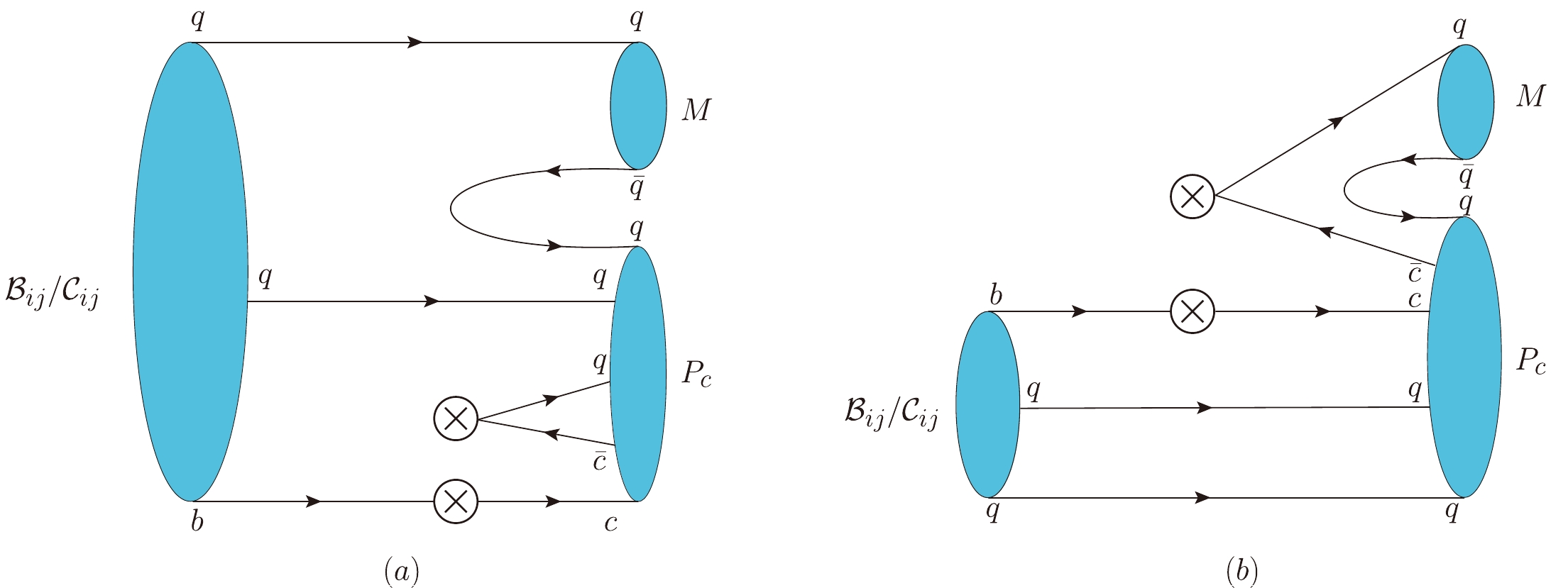
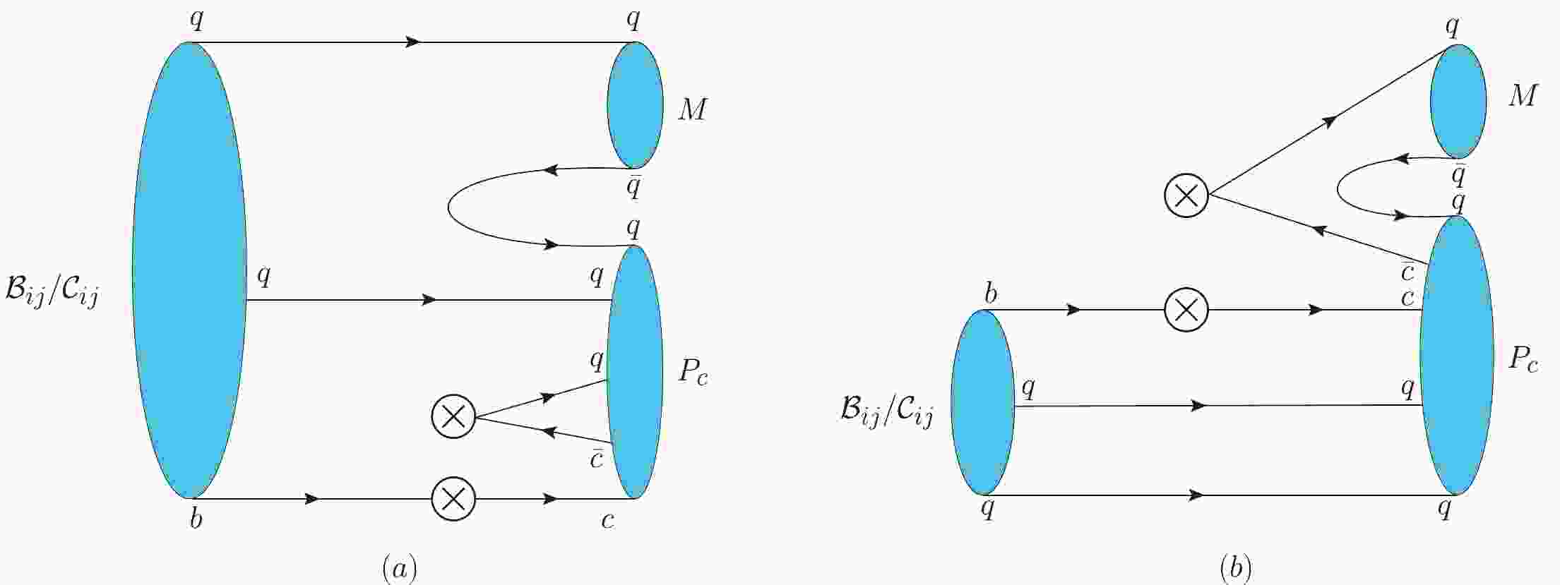
Figure 1. (color online) Topological diagrams for b-baryon decays into an octet pentaquark and a light meson. Panel (a) corresponds to terms
$ a_{3} $ ,$ a_{4} $ ,$ a_{5} $ and$ b_{2} $ ,$ b_{3} $ ,$ b_{4} $ in Eqs. (12) and (13), respectively. Panel (b) corresponds to terms$ a_{1} $ ,$ a_{2} $ , and$ b_{1} $ .channel amplitude channel amplitude $ \Lambda_b^0\to P_{\Sigma^-} \pi^+ $ 

$ \left(a_3-a_2\right) V_{\text{cs}}^* $ 

$ \Lambda_b^0\to P_{\Sigma^-} K^+ $ 

$ -a_3 V_{\text{cd}}^* $ 

$ \Lambda_b^0\to P_{\Sigma^0} \pi^0 $ 

$ \left(a_3-a_2\right) V_{\text{cs}}^* $ 

$ \Lambda_b^0\to P_{\Sigma^0} K^0 $ 

$ \dfrac{a_3}{\sqrt{2}}V_{\text{cd}}^* $ 

$ \Lambda_b^0\to P_{\Sigma^+} \pi^- $ 

$ \left(a_3-a_2\right) V_{\text{cs}}^* $ 

$ \Lambda_b^0\to P_{p} \pi^- $ 

$ \left(a_1+a_2-a_3\right) V_{\text{cd}}^* $ 

$ \Lambda_b^0\to P_{p} K^- $ 

$ a_1 V_{\text{cs}}^* $ 

$ \Lambda_b^0\to P_{n} \pi^0 $ 

$ -\dfrac{\left(a_1+a_2-a_3\right) }{\sqrt{2}}V_{\text{cd}}^* $ 

$ \Lambda_b^0\to P_{n} \overline K^0 $ 

$ a_1 V_{\text{cs}}^* $ 

$ \Lambda_b^0\to P_{\Lambda} K^0 $ 

$ -\dfrac{\left(2 a_1+2 a_2-a_3\right) }{\sqrt{6}}V_{\text{cd}}^* $ 

$ \Xi_b^0\to P_{\Lambda} \overline K^0 $ 

$ -\dfrac{\left(a_1+a_2+a_3\right) }{\sqrt{6}}V_{\text{cs}}^* $ 

$ \Xi_b^0\to P_{\Sigma^0} \pi^0 $ 

$ \dfrac{\left(-a_1+a_2\right)}{2} V_{\text{cd}}^* $ 

$ \Xi_b^0\to P_{\Sigma^0} \overline K^0 $ 

$ \dfrac{\left(a_1+a_2-a_3\right) }{\sqrt{2}}V_{\text{cs}}^* $ 

$ \Xi_b^0\to P_{\Sigma^+} \pi^- $ 

$ -a_1 V_{\text{cd}}^* $ 

$ \Xi_b^0\to P_{\Sigma^+} K^- $ 

$ -\left(a_1+a_2-a_3\right) V_{\text{cs}}^* $ 

$ \Xi_b^0\to P_{p} K^- $ 

$ \left(a_2-a_3\right) V_{\text{cd}}^* $ 

$ \Xi_b^-\to P_{\Lambda} K^- $ 

$ \dfrac{\left(a_1+a_2+a_3\right) }{\sqrt{6}}V_{\text{cs}}^* $ 

$ \Xi_b^0\to P_{\Lambda} \pi^0 $ 

$ \dfrac{\left(a_1+a_2-2 a_3\right) }{2 \sqrt{3}}V_{\text{cd}}^* $ 

$ \Xi_b^-\to P_{\Sigma^-} \overline K^0 $ 

$ \left(a_1+a_2-a_3\right) V_{\text{cs}}^* $ 

$ \Xi_b^0\to P_{n} \overline K^0 $ 

$ a_2 V_{\text{cd}}^* $ 

$ \Xi_b^-\to P_{\Sigma^0} K^- $ 

$ \dfrac{\left(a_1+a_2-a_3\right) }{\sqrt{2}}V_{\text{cs}}^* $ 

$ \Xi_b^-\to P_{\Lambda} \pi^- $ 

$ \dfrac{\left(a_1+a_2-2 a_3\right) }{\sqrt{6}}V_{\text{cd}}^* $ 

$ \Xi_b^-\to P_{\Sigma^-} \pi^0 $ 

$ -\dfrac{\left(a_1+a_2\right)}{\sqrt{2}} V_{\text{cd}}^* $ 

$ \Xi_b^0\to P_{\Sigma^-} \pi^+ $ 

$ a_2 V_{\text{cd}}^* $ 

$ \Xi_b^-\to P_{n} K^- $ 

$ -a_3 V_{\text{cd}}^* $ 

$ \Xi_b^-\to P_{\Sigma^0} \pi^- $ 

$ \dfrac{\left(a_1+a_2\right) }{\sqrt{2}}V_{\text{cd}}^* $ 

Table 1. Amplitudes for b-baryon (antitriplet) decays into a pentaquark and a light meson.
channel amplitude channel amplitude $ \Sigma_{b}^{+}\to P_{\Lambda} \pi^+ $ 

$ -\dfrac{\left(b_2+b_3\right)}{\sqrt{6}} V_{\text{cs}}^* $ 

$ \Sigma_{b}^{+}\to P_{\Lambda} K^+ $ 

$ \dfrac{\left(-2 b_2+b_3\right)}{\sqrt{6}} V_{\text{cd}}^* $ 

$ \Sigma_{b}^{+}\to P_{\Sigma^0} \pi^+ $ 

$ \dfrac{\left(b_2-b_3\right) }{\sqrt{2}}V_{\text{cs}}^* $ 

$ \Sigma_{b}^{+}\to P_{\Sigma^0} K^+ $ 

$ \dfrac{b_3}{\sqrt{2}}V_{\text{cd}}^* $ 

$ \Sigma_{b}^{+}\to P_{\Sigma^+} \pi^0 $ 

$ \dfrac{\left(b_3-b_2\right) }{\sqrt{2}}V_{\text{cs}}^* $ 

$ \Sigma_{b}^{+}\to P_{\Sigma^+} K^0 $ 

$ -b_1 V_{\text{cd}}^* $ 

$ \Sigma_{b}^{+}\to P_{p} \overline K^0 $ 

$ b_1 V_{\text{cs}}^* $ 

$ \Sigma_{b}^{+}\to P_{n} \pi^+ $ 

$ b_2 V_{\text{cd}}^* $ 

$ \Sigma_{b}^{0}\to P_{\Lambda} \pi^0 $ 

$ \dfrac{\left(b_2+b_3\right) }{\sqrt{6}}V_{\text{cs}}^* $ 

$ \Sigma_{b}^{0}\to P_{\Lambda} K^0 $ 

$ -\dfrac{\left(2 b_2-b_3\right) }{2 \sqrt{3}}V_{\text{cd}}^* $ 

$ \Sigma_{b}^{0}\to P_{\Sigma^-} \pi^+ $ 

$ \dfrac{\left(b_2-b_3\right) }{\sqrt{2}}V_{\text{cs}}^* $ 

$ \Sigma_{b}^{0}\to P_{\Sigma^-} K^+ $ 

$ \dfrac{b_3}{\sqrt{2}}V_{\text{cd}}^* $ 

$ \Sigma_{b}^{0}\to P_{\Sigma^+} \pi^- $ 

$ \dfrac{\left(b_3-b_2\right) }{\sqrt{2}}V_{\text{cs}}^* $ 

$ \Sigma_{b}^{+}\to P_{p} \pi^0 $ 

$ -\dfrac{\left(b_1-b_2+b_3\right) }{\sqrt{2}}V_{\text{cd}}^* $ 

Continued on next page Table 2. Amplitudes for b-baryon (sextet) decays into a pentaquark and a light meson.
Table 2-continued from previous page channel amplitude channel amplitude $ \Sigma_{b}^{0}\to P_{p} K^- $ 

$ -\dfrac{b_1}{\sqrt{2}}V_{\text{cs}}^* $ 

$ \Sigma_{b}^{0}\to P_{\Sigma^0} K^0 $ 

$ \dfrac{\left(2 b_1+b_3\right)}{2} V_{\text{cd}}^* $ 

$ \Sigma_{b}^{0}\to P_{n} \overline K^0 $ 

$ \dfrac{b_1}{\sqrt{2}}V_{\text{cs}}^* $ 

$ \Sigma_{b}^{0}\to P_{p} \pi^- $ 

$ -\dfrac{\left(b_1-b_2+b_3\right) }{\sqrt{2}}V_{\text{cd}}^* $ 

$ \Sigma_{b}^{-}\to P_{\Lambda} \pi^- $ 

$ \dfrac{\left(b_2+b_3\right) }{\sqrt{6}}V_{\text{cs}}^* $ 

$ \Sigma_{b}^{0}\to P_{n} \pi^0 $ 

$ -\dfrac{\left(b_1+b_2+b_3\right)}{2} V_{\text{cd}}^* $ 

$ \Sigma_{b}^{-}\to P_{\Sigma^-} \pi^0 $ 

$ \dfrac{\left(b_3-b_2\right) }{\sqrt{2}}V_{\text{cs}}^* $ 

$ \Sigma_{b}^{-}\to P_{\Sigma^-} K^0 $ 

$ \left(b_1+b_3\right) V_{\text{cd}}^* $ 

$ \Sigma_{b}^{-}\to P_{\Sigma^0} \pi^- $ 

$ \dfrac{\left(b_2-b_3\right) }{\sqrt{2}}V_{\text{cs}}^* $ 

$ \Sigma_{b}^{-}\to P_{n} \pi^- $ 

$ -\left(b_1+b_3\right) V_{\text{cd}}^* $ 

$ \Sigma_{b}^{-}\to P_{n} K^- $ 

$ -b_1 V_{\text{cs}}^* $ 

$ \Xi_{b}^{\prime0}\to P_{\Lambda} \pi^0 $ 

$ \dfrac{\left(3 b_1-b_2+2 b_3\right) }{2 \sqrt{6}}V_{\text{cd}}^* $ 

$ \Xi_{b}^{\prime0}\to P_{\Lambda} \overline K^0 $ 

$ -\dfrac{\left(3 b_1+b_2+b_3\right) }{2 \sqrt{3}}V_{\text{cs}}^* $ 

$ \Xi_{b}^{\prime0}\to P_{\Sigma^-} \pi^+ $ 

$ -\dfrac{b_2}{\sqrt{2}}V_{\text{cd}}^* $ 

$ \Xi_{b}^{\prime0}\to P_{\Sigma^0} \overline K^0 $ 

$ -\dfrac{\left(b_1-b_2+b_3\right)}{2} V_{\text{cs}}^* $ 

$ \Xi_{b}^{\prime0}\to P_{\Sigma^0} \pi^0 $ 

$ \dfrac{\left(b_1-b_2\right) }{2 \sqrt{2}}V_{\text{cd}}^* $ 

$ \Xi_{b}^{\prime0}\to P_{\Sigma^+} K^- $ 

$ \dfrac{\left(b_1-b_2+b_3\right) }{\sqrt{2}}V_{\text{cs}}^* $ 

$ \Xi_{b}^{\prime0}\to P_{\Sigma^+} \pi^- $ 

$ \dfrac{b_1}{\sqrt{2}}V_{\text{cd}}^* $ 

$ \Xi_{b}^{\prime-}\to P_{\Lambda} K^- $ 

$ \dfrac{\left(3 b_1+b_2+b_3\right) }{2 \sqrt{3}}V_{\text{cs}}^* $ 

$ \Xi_{b}^{\prime0}\to P_{p} K^- $ 

$ \dfrac{\left(b_2-b_3\right) }{\sqrt{2}}V_{\text{cd}}^* $ 

$ \Xi_{b}^{\prime-}\to P_{\Sigma^-} \overline K^0 $ 

$ -\dfrac{\left(b_1-b_2+b_3\right) }{\sqrt{2}}V_{\text{cs}}^* $ 

$ \Xi_{b}^{\prime0}\to P_{n} \overline K^0 $ 

$ \dfrac{b_2}{\sqrt{2}}V_{\text{cd}}^* $ 

$ \Xi_{b}^{\prime-}\to P_{\Sigma^0} K^- $ 

$ -\dfrac{\left(b_1-b_2+b_3\right)}{2} V_{\text{cs}}^* $ 

$ \Xi_{b}^{\prime-}\to P_{\Lambda} \pi^- $ 

$ \dfrac{\left(3 b_1-b_2+2 b_3\right) }{2 \sqrt{3}}V_{\text{cd}}^* $ 

$ \Xi_{b}^{\prime-}\to P_{\Sigma^-} \pi^0 $ 

$ \dfrac{\left(b_1+b_2\right)}{2} V_{\text{cd}}^* $ 

$ \Xi_{b}^{\prime-}\to P_{\Sigma^0} \pi^- $ 

$ -\dfrac{\left(b_1+b_2\right)}{2} V_{\text{cd}}^* $ 

$ \Xi_{b}^{\prime-}\to P_{n} K^- $ 

$ -\dfrac{b_3}{\sqrt{2}}V_{\text{cd}}^* $ 

$ \Omega_{b}^{-}\to P_{\Lambda} K^- $ 

$ \dfrac{\left(-b_2+2 b_3\right) }{\sqrt{6}}V_{\text{cd}}^* $ 

$ \Omega_{b}^{-}\to P_{\Sigma^-} \overline K^0 $ 

$ -b_2 V_{\text{cd}}^* $ 

$ \Omega_{b}^{-}\to P_{\Sigma^0} K^- $ 

$ -\dfrac{b_2}{\sqrt{2}}V_{\text{cd}}^* $ 

1. Tables 1 and 2 are arranged according to the dependence on the CKM matrix elements; the
$ c\to s $ transition is proportional to$ |V_{cs}^*|\sim 1 $ , whereas the$ c\to d $ transition is Cabibbo-suppressed$ |V_{cd}^*|\sim 0.2 $ .2. A number of relations for different decay widths can be readily extracted from Table 1:
$\begin{aligned}[b]{{\Gamma}}\left({{\Lambda}}_{{b}}^{{0}} \rightarrow {{P}}_{{p}} {{K}}^-\right)=\;&{{\Gamma}}\left({{\Lambda}}_{{b}}^{{0}} \rightarrow {{P}}_{{n}} \bar{{{K}}}^{{0}}\right), \\ {{\Gamma}}\left({{\Lambda}}_{{b}}^{{0}} \rightarrow {{P}}_{{p}} {{\pi}}^-\right)=\;&2 {{\Gamma}}\left({{\Lambda}}_{{b}}^{{0}} \rightarrow {{P}}_{{n}} {{\pi}}^{{0}}\right), \\ {{\Gamma}}\left({{\Lambda}}_{{b}}^{{0}} \rightarrow {{P}}_{{{\Sigma}}^-} {{K}}^+\right)=\;&2 {{\Gamma}}\left({{\Lambda}}_{{b}}^{{0}} \rightarrow {{P}}_{{{\Sigma}}^{{0}}} {{K}}^{{0}}\right), \\ {{\Gamma}}\left({{\Lambda}}_{{b}}^{{0}} \rightarrow {{P}}_{{{\Sigma}}^-} {{\pi}}^+\right)=\;&{{\Gamma}}\left({{\Lambda}}_{{b}}^{{0}} \rightarrow {{P}}_{{{\Sigma}}^+} {{\pi}}^-\right) \\ =\;&{{\Gamma}}\left({{\Lambda}}_{{b}}^{{0}} \rightarrow {{P}}_{{{\Sigma}}^{{0}}} {{\pi}}^{{0}}\right), \\ {{\Gamma}}\left({{\Xi}}_{{b}}^{{0}} \rightarrow {{P}}_{{{\Lambda}}} \bar{{{K}}}^{{0}}\right)=\;&{{\Gamma}}\left({{\Xi}}_{{b}}^- \rightarrow {{P}}_{{{\Lambda}}} {{K}}^-\right), \\ {{\Gamma}}\left({{\Xi}}_{{b}}^- \rightarrow {{P}}_{{{\Sigma}}^-} {{\pi}}^{{0}}\right)=\;&{{\Gamma}}\left({{\Xi}}_{{b}}^- \rightarrow {{P}}_{{{\Sigma}}^{{0}}} {{\pi}}^-\right), \\ {{\Gamma}}\left({{\Xi}}_{{b}}^- \rightarrow {{P}}_{{{\Lambda}}} {{\pi}}^-\right)=\;&2 {{\Gamma}}\left({{\Xi}}_{{b}}^{{0}} \rightarrow {{P}}_{{{\Lambda}}} {{\pi}}^{{0}}\right), \\ {{\Gamma}}\left({{\Xi}}_{{b}}^- \rightarrow {{P}}_{{{\Sigma}}^-} \bar{{{K}}}^{{0}}\right)=\;&{{\Gamma}}\left({{\Xi}}_{{b}}^{{0}} \rightarrow {{P}}_{{{\Sigma}}^+} {{K}}^-\right) \\ =\;&2 {{\Gamma}}\left({{\Xi}}_{{b}}^{{0}} \rightarrow {{P}}_{{{\Sigma}}^{{0}}} \bar{{{K}}}^{{0}}\right), \\ =\;&2 {{\Gamma}}\left({{\Xi}}_{{b}}^- \rightarrow {{P}}_{{{\Sigma}}^{{0}}} {{K}}^-\right), \\ \Gamma\left(\Lambda_b^0 \rightarrow P_{\Sigma^-} K^+\right)=\;&\Gamma\left(\Xi_b^- \rightarrow P_n K^-\right), \\ \Gamma\left(\Xi_b^0 \rightarrow P_{\Sigma^-} \pi^+\right)=\;&\Gamma\left(\Xi_b^0 \rightarrow P_n \bar{K}^0\right) .\end{aligned}$

(14) Likewise, the following relations can be deduced from Table 2:
$ \begin{aligned}[b] {{\Gamma}}({{\Omega}}_{{b}}^-\to {{P}}_{{{\Sigma}}^-} \overline {{K}}^{{0}} ) =\;& 2{{\Gamma}}({{\Omega}}_{{b}}^-\to {{P}}_{{{\Sigma}}^{{0}}} {{K}}^- ) \, , \\ {{\Gamma}}({{\Xi}}_{{b}}^{\prime{{0}}}\to {{P}}_{{{\Lambda}}} \overline {{K}}^{{0}} ) =\;& {{\Gamma}}({{\Xi}}_{{b}}^{\prime-}\to {{P}}_{{{\Lambda}}} {{K}}^- ) \, , \\ {{\Gamma}}({{\Xi}}_{{b}}^{\prime{{0}}}\to {{P}}_{{{\Sigma}}^+} {{K}}^- ) =\;& {{\Gamma}}({{\Xi}}_{{b}}^{\prime-}\to {{P}}_{{{\Sigma}}^-} \overline {{K}}^{{0}} ) \\ =\;&{{ 2{{\Gamma}}({{\Xi}}_{{b}}^{\prime{{0}}}\to {{P}}_{{{\Sigma}}^{{0}}} \overline {{K}}^{{0}} )}} \\ =\;&{{ 2{{\Gamma}}({{\Xi}}_{{b}}^{\prime-}\to {{P}}_{{{\Sigma}}^{{0}}} {{K}}^- ) \, , }} \\ {{\Gamma}}({{\Xi}}_{{b}}^{\prime-}\to {{P}}_{{{\Lambda}}} {{\pi}}^- ) =\;& 2{{\Gamma}}({{\Xi}}_{{b}}^{\prime{{0}}}\to {{P}}_{{{\Lambda}}} {{\pi}}^{{0}} ) \, , \\ {{\Gamma}}({{\Xi}}_{{b}}^{\prime-}\to {{P}}_{{{\Sigma}}^-} {{\pi}}^{{0}} ) =\;& {{\Gamma}}({{\Xi}}_{{b}}^{\prime-}\to {{P}}_{{{\Sigma}}^{{0}}} {{\pi}}^- ) \, , \\ {{\Gamma}}({{\Sigma}}_{{b}}^+\to {{P}}_{{{\Lambda}}} {{\pi}}^+ ) =\;& {{\Gamma}}({{\Sigma}}_{{b}}^-\to {{P}}_{{{\Lambda}}} {{\pi}}^- ) \, , \\ {{\Gamma}}({{\Sigma}}_{{b}}^+\to {{P}}_{{{\Sigma}}^{{0}}} {{\pi}}^+ ) =\;& {{\Gamma}}({{\Sigma}}_{{b}}^-\to {{P}}_{{{\Sigma}}^{{0}}} {{\pi}}^- ) \, , \\ {{\Gamma}}({{\Sigma}}_{{b}}^+\to {{P}}_{{p}} \overline {{K}}^{{0}} ) =\;& {{\Gamma}}({{\Sigma}}_{{b}}^-\to {{P}}_{n} {{K}}^- ) \, , \\ {{\Gamma}}({{\Sigma}}_{{b}}^+\to {{P}}_{{{\Lambda}}} {{\pi}}^+ ) =\;& {{\Gamma}}({{\Sigma}}_{{b}}^{{{0}}}\to {{P}}_{{{\Lambda}}} {{\pi}}^{{0}} ) \, , \\ {{\Gamma}}({{\Sigma}}_{{b}}^+\to {{P}}_{{{\Lambda}}} {{K}}^+ ) =\;& 2{{\Gamma}}({{\Sigma}}_{{b}}^{{{0}}}\to {{P}}_{{{\Lambda}}} {{K}}^{{0}} ) \, , \end{aligned} $

$ \begin{aligned}[b] {{\Gamma}}({{\Sigma}}_{{b}}^+\to {{P}}_{{{\Sigma}}^{{0}}} {{K}}^+ ) =\;& {{\Gamma}}({{\Sigma}}_{{b}}^{{{0}}}\to {{P}}_{{{\Sigma}}^-} {{K}}^+ ) \, , \\ {{\Gamma}}({{\Sigma}}_{{b}}^+\to {{P}}_{{p}} {{\pi}}^{{0}} ) =\;& {{\Gamma}}({{\Sigma}}_{{b}}^{{{0}}}\to {{P}}_{{p}} {{\pi}}^- ) \, , \\ {{\Gamma}}({{\Sigma}}_{{b}}^+\to {{P}}_{{p}} \overline {{K}}^{{0}} ) =\;& 2{{\Gamma}}({{\Sigma}}_{{b}}^{{{0}}}\to {{P}}_{n} \overline {{K}}^{{0}} ) \\ =\;&{{ 2{{\Gamma}}({{\Sigma}}_{{b}}^{{{0}}}\to {{P}}_{{p}} {{K}}^- ) \, , }} \\ {{\Gamma}}({{\Sigma}}_{{b}}^+\to {{P}}_{{{\Sigma}}^{{0}}} {{\pi}}^+ ) =\;& {{\Gamma}}({{\Sigma}}_{{b}}^+\to {{P}}_{{{\Sigma}}^+} {{\pi}}^{{0}} ) \\ =\;&{{ {{\Gamma}}({{\Sigma}}_{{b}}^{{{0}}}\to {{P}}_{{{\Sigma}}^+} {{\pi}}^- )}}\\ =\;&{{ {{\Gamma}}({{\Sigma}}_{{b}}^{{{0}}}\to {{P}}_{{{\Sigma}}^-} {{\pi}}^+ )}}\\ =\;&{{ {{\Gamma}}({{\Sigma}}_{{b}}^-\to {{P}}_{{{\Sigma}}^-} {{\pi}}^{{0}} ) \, , }} \\ {{\Gamma}}({{\Sigma}}_{{b}}^{{{0}}}\to {{P}}_{{{\Lambda}}} {{\pi}}^{{0}} ) =\;& {{\Gamma}}({{\Sigma}}_{{b}}^-\to {{P}}_{{{\Lambda}}} {{\pi}}^- ) \, , \\ \Gamma(\Omega_{b}^-\to P_{\Sigma^-} \overline K^0 ) =\;&\Gamma(\Sigma_{b}^+\to P_{n} \pi^+ ) \\ =\;&2\Gamma(\Xi_{b}^{\prime0}\to P_{n} \overline K^0 )\\ =\;&2\Gamma(\Xi_{b}^{\prime0}\to P_{\Sigma^-} \pi^+ ) \, , \\ \Gamma(\Sigma_{b}^+\to P_{\Sigma^0} K^+ ) =\;&\Gamma(\Xi_{b}^{\prime-}\to P_{n} K^- ) \\ \Gamma(\Sigma_{b}^+\to P_{\Sigma^+} K^0 ) =\;&2\Gamma(\Xi_{b}^{\prime0}\to P_{\Sigma^+} \pi^- ) \, , \\ \Gamma(\Sigma_{b}^-\to P_{\Sigma^-} K^0 ) =\;&\Gamma(\Sigma_{b}^-\to P_{n} \pi^- ) \, . \end{aligned} $

(15) The relations marked in bold are upheld by the I-spin symmetry; they are more reliable than the U- and V-spin relations. The abovementioned results constitute the relative relations; absolute decay rates require a reliable computation of the irreducible nonperturbative amplitudes. However, this is a daunting task, notably beyond the theoretical methods presently available. Moreover, the decay modes of
$ \Omega_b^- $ might be experimentally more important, given that the decays of$ \Sigma_b $ and$ \Xi_{b} $ are dominated by strong interactions.3. Let us take
$ P_c(4312) $ as$ P_p $ and$ P_{cs}(4459) $ as$ P_{\Lambda} $ in Eq. (3) according to the different light valence quark components. Then, some of the abovementioned relations facilitate the exploration of new decay modes. Combined with the strong decays of pentaquarks, we next report on some cascade decay modes that are likely to be utilized to reconstruct the pentaquarks.However, it is necessary to point out that the abovementioned relations between decay widths are only an estimate because they were obtained in the flavor
$S U(3) $ symmetry limit, in which the mass differences between final state hadrons have been ignored. In addition, the hadronization processes influence the relations derived in this study. Although the$S U(3) $ breaking effects might be sizable, our qualitative results should be relatively robust, unless the flavor symmetry is broken in a much stronger manner in bottom quark decays than empirically anticipated. With more data from LCHb and other experiments in the future, a rigorous analysis will be necessary [58, 59]. -
At the hadron level, for a B-meson which belongs to an
$S U(3) $ antitriplet decay into an octet pentaquark and a light antibaryon, the corresponding effective Hamiltonian is constructed as$\begin{aligned}[b]{\cal H}_{\rm eff}=\;& c_1 (B)_n (H)^n \epsilon_{ijk} ({\cal{\overline{P}}})^k_l \epsilon^{ilm} (T_8)^j_m \\ &+ c_2 (B)_n (H)^l \epsilon_{ijk} ({\cal{\overline{P}}})^k_l \epsilon^{inm} (T_8)^j_m \\ &+ c_3 (B)_n (H)^j \epsilon_{ijk} ({\cal{\overline{P}}})^k_l \epsilon^{inm} (T_8)^l_m \, .\end{aligned}$

(16) The topological diagrams for these decays are presented in Fig. 2. The decay amplitudes for different channels can be deduced from the Hamiltonian in Eq. (16); they are listed in Table 3. From these amplitudes, we can find the relations for decay widths in the
$S U(3) $ symmetry limit: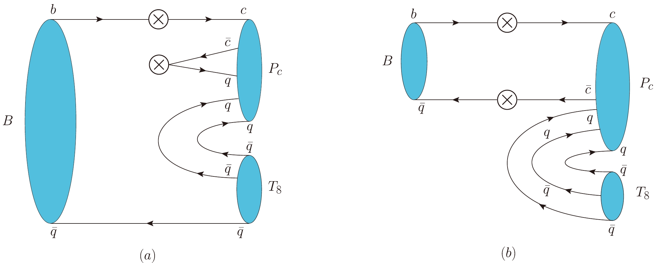
Figure 2. (color online) Topological diagrams for a B-meson decay into an octet pentaquark and a light antibaryon. Panel (a) refers to terms
$ c_{2} $ and$ c_{3} $ whereas panel (b) refers to term$ c_{1} $ in Eq. (16).channel amplitude channel amplitude $ B^-\to P_{\Lambda} \overline p $ 

$ -\dfrac{\left(2 c_2+c_3\right) }{\sqrt{6}}V_{\text{cs}}^* $ 

$ B^-\to P_{\Sigma^-} \overline \Lambda^0 $ 

$ \dfrac{\left(c_2-c_3\right) }{\sqrt{6}}V_{\text{cd}}^* $ 

$ B^-\to P_{\Sigma^-} \overline n $ 

$ -c_3 V_{\text{cs}}^* $ 

$ B^-\to P_{\Lambda} \overline \Sigma^- $ 

$ \dfrac{\left(c_2-c_3\right) }{\sqrt{6}}V_{\text{cd}}^* $ 

$ B^-\to P_{\Sigma^0} \overline p $ 

$ -\dfrac{c_3}{\sqrt{2}}V_{\text{cs}}^* $ 

$ B^-\to P_{\Sigma^-} \overline \Sigma^0 $ 

$ \dfrac{\left(c_2+c_3\right) }{\sqrt{2}}V_{\text{cd}}^* $ 

$ \overline B^0\to P_{\Lambda} \overline n $ 

$ -\dfrac{\left(2 c_2+c_3\right) }{\sqrt{6}}V_{\text{cs}}^* $ 

$ B^-\to P_{\Sigma^0} \overline \Sigma^- $ 

$ -\dfrac{\left(c_2+c_3\right) }{\sqrt{2}}V_{\text{cd}}^* $ 

$ \overline B^0\to P_{\Sigma^0} \overline n $ 

$ \dfrac{c_3}{\sqrt{2}}V_{\text{cs}}^* $ 

$ B^-\to P_{n} \overline p $ 

$ c_2 V_{\text{cd}}^* $ 

$ \overline B^0\to P_{\Sigma^+} \overline p $ 

$ -c_3 V_{\text{cs}}^* $ 

$ \overline B^0\to P_{\Lambda} \overline \Lambda^0 $ 

$ \dfrac{\left(6 c_1+c_2+5 c_3\right)}{6} V_{\text{cd}}^* $ 

$ \overline B^0_s\to P_{\Lambda} \overline \Lambda^0 $ 

$ \dfrac{\left(3 c_1+2 c_2+c_3\right)}{3} V_{\text{cs}}^* $ 

$ \overline B^0\to P_{\Lambda} \overline \Sigma^0 $ 

$ -\dfrac{\left(c_2-c_3\right) }{2 \sqrt{3}}V_{\text{cd}}^* $ 

$ \overline B^0_s\to P_{\Sigma^-} \overline \Sigma^+ $ 

$ \left(c_1+c_3\right) V_{\text{cs}}^* $ 

$ \overline B^0\to P_{\Sigma^-} \overline \Sigma^+ $ 

$ \left(c_1+c_2+c_3\right) V_{\text{cd}}^* $ 

$ \overline B^0_s\to P_{\Sigma^0} \overline \Sigma^0 $ 

$ \left(c_1+c_3\right) V_{\text{cs}}^* $ 

$ \overline B^0\to P_{\Sigma^0} \overline \Lambda^0 $ 

$ -\dfrac{\left(c_2-c_3\right)}{2 \sqrt{3}} V_{\text{cd}}^* $ 

$ \overline B^0_s\to P_{\Sigma^+} \overline \Sigma^- $ 

$ \left(c_1+c_3\right) V_{\text{cs}}^* $ 

$ \overline B^0\to P_{\Sigma^0} \overline \Sigma^0 $ 

$ \dfrac{\left(2 c_1+c_2+c_3\right)}{2} V_{\text{cd}}^* $ 

$ \overline B^0_s\to P_{p} \overline p $ 

$ c_1 V_{\text{cs}}^* $ 

$ \overline B^0\to P_{\Sigma^+} \overline \Sigma^- $ 

$ c_1 V_{\text{cd}}^* $ 

$ \overline B^0_s\to P_{n} \overline n $ 

$ c_1 V_{\text{cs}}^* $ 

$ \overline B^0\to P_{p} \overline p $ 

$ \left(c_1+c_2\right) V_{\text{cd}}^* $ 

$ \overline B^0\to P_{n} \overline n $ 

$ \left(c_1+c_2+c_3\right) V_{\text{cd}}^* $ 

$ \overline B^0_s\to P_{\Lambda} \overline \Xi^0 $ 

$ \dfrac{\left(c_2+2 c_3\right) }{\sqrt{6}}V_{\text{cd}}^* $ 

$ \overline B^0_s\to P_{\Sigma^-} \overline \Xi^+ $ 

$ c_2 V_{\text{cd}}^* $ 

$ \overline B^0_s\to P_{\Sigma^0} \overline \Xi^0 $ 

$ -\dfrac{c_2}{\sqrt{2}}V_{\text{cd}}^* $ 

$ \overline B^0_s\to P_{p} \overline \Sigma^- $ 

$ -c_3 V_{\text{cd}}^* $ 

$ \overline B^0_s\to P_{n} \overline \Lambda^0 $ 

$ -\dfrac{\left(2 c_2+c_3\right) }{\sqrt{6}}V_{\text{cd}}^* $ 

$ \overline B^0_s\to P_{n} \overline \Sigma^0 $ 

$ \dfrac{c_3}{\sqrt{2}} V_{\text{cd}}^* $ 

Table 3. Amplitudes for B-meson decays into a pentaquark and a light baryon.
$ \begin{aligned}[b] \Gamma(B^-\to P_{\Lambda} \overline \Sigma^-) =\;& \Gamma(B^-\to P_{\Sigma^-} \overline \Lambda^0) \\ =\;& 2\Gamma(\overline B^0\to P_{\Lambda} \overline \Sigma^0) \\ =\;& 2\Gamma(\overline B^0\to P_{\Sigma^0} \overline \Lambda^0) \, , \\ \Gamma(B^-\to P_{\Sigma^-} \overline \Sigma^0) =\;& \Gamma (B^-\to P_{\Sigma^0} \overline \Sigma^- ) \, , \\ \Gamma(B^-\to P_{\Sigma^-} \overline n) =\;& \Gamma(\overline B^0\to P_{\Sigma^+} \overline p) \\ =\;& 2\Gamma(\overline B^0\to P_{\Sigma^0} \overline n) \\ =\;& 2\Gamma(B^-\to P_{\Sigma^0} \overline p) \, , \\ \Gamma(B^-\to P_{\Lambda} \overline p)=\;& \Gamma(\overline B^0\to P_{\Lambda} \overline n) \, , \\ \Gamma(\overline B^0_s\to P_{p} \overline \Sigma^-) =\;& 2\Gamma(\overline B^0_s\to P_{n} \overline \Sigma^0) \, , \\ \Gamma(\overline B^0\to P_{\Sigma^-} \overline \Sigma^+) =\;& \Gamma(\overline B^0\to P_{n} \overline n) \, , \\ \Gamma(\overline B^0_s\to P_{\Sigma^-} \overline \Sigma^+) =\;& \Gamma(\overline B^0_s\to P_{\Sigma^0} \overline \Sigma^0) \\ =\;& \Gamma(\overline B^0_s\to P_{\Sigma^+} \overline \Sigma^-) \, , \\ \Gamma(\overline B^0_s\to P_{\Sigma^-} \overline \Xi^+) =\;& \Gamma(B^-\to P_{n} \overline p) \\ =\;& 2\Gamma(\overline B^0_s\to P_{\Sigma^0} \overline \Xi^0) \, , \\ \Gamma(\overline B^0_s\to P_{p} \overline p) =\;& \Gamma(\overline B^0_s\to P_{n} \overline n) \, .\end{aligned} $

(17) Amplitude analyses of
$ B_s^0 \to J/\psi \, p \, \bar p $ and$ B^- \to J/\psi \Lambda \, \overline{p} $ were recently performed by the LHCb Collaboration, and evidences for charmonium pentaquarks were reported. Unlike baryonic decays, mesonic decays offer a cleaner environment to search for new pentaquarks. The relations in Eq. (17) can be utilized to find new decay channels; for instance, Cabibbo-allowed processes$ \overline B^0\to P_{\Lambda} \overline n $ ,$ \overline B^0\to P_{\Sigma^+} \overline p $ , and$ \overline B^0_s\to P_{n} \overline n $ have the potential to be experimentally discovered in the future. -
The particular decay processes of
$ P_c $ states in the detectors can be adapted as signatures to reconstruct these exotic states. Currently, the experimental searches for pentaquarks mainly focus on the strong decays of$ P_c $ ; this is the case of$ P_c(4312) \to J/\psi \, p $ [6] and$ P_{cs}(4459) \to J/\psi \Lambda $ [7]. The effective Hamiltonian for an octet pentaquark decay into$ J/\psi $ plus a light baryon is expressed as$ {\cal H}_{\rm eff}= d_1 \epsilon^{ijk} ({\cal{P}})^l_k \epsilon_{ilm} (\overline{T}_8)^m_j J/\psi \, . $

(18) These processes belong to strong decays. Therefore, there are no effective vertices; this is a unique property compared with the weak decays of a b-baryon and B-meson. The decay amplitudes deduced from Eq. (18) are presented in Table 4, showing that all the decay widths are the same:
channel amplitude channel amplitude $ P_{\Lambda}\to \Lambda^0 J/\psi $ 

$ -d_1 $ 

$ P_{\Sigma^-}\to \Sigma^+ J/\psi $ 

$ -d_1 $ 

$ P_{\Sigma^0}\to \Sigma^0 J/\psi $ 

$ -d_1 $ 

$ P_{\Sigma^+}\to \Sigma^- J/\psi $ 

$ -d_1 $ 

$ P_{p}\to \Xi^- J/\psi $ 

$ -d_1 $ 

$ P_{n}\to \Xi^0 J/\psi $ 

$ -d_1 $ 

$ P_{\Lambda}\to \Lambda_c^+ D^-_s $ 

$ -\sqrt{\dfrac{2}{3}} e_1 $ 

$ P_{\Lambda}\to \Xi_{c}^{\prime+} D^- $ 

$ -\dfrac{\sqrt{3}}{2} e_2 $ 

$ P_{\Lambda}\to \Xi_c^+ D^- $ 

$ -\dfrac{e_1}{\sqrt{6}} $ 

$ P_{n}\to \Sigma_{c}^{0} \overline D^0 $ 

$ -e_2 $ 

$ P_{\Lambda}\to \Xi_c^0 \overline D^0 $ 

$ \dfrac{e_1}{\sqrt{6}} $ 

$ P_{\Lambda}\to \Xi_{c}^{\prime0} \overline D^0 $ 

$ \dfrac{\sqrt{3} e_2}{2} $ 

$ P_{\Sigma^-}\to \Xi_c^0 D^- $ 

$ e_1 $ 

$ P_{\Sigma^-}\to \Sigma_{c}^{0} D^-_s $ 

$ e_2 $ 

$ P_{\Sigma^0}\to \Xi_c^+ D^- $ 

$ \dfrac{e_1}{\sqrt{2}} $ 

$ P_{\Sigma^-}\to \Xi_{c}^{\prime0} D^- $ 

$ -\dfrac{e_2}{\sqrt{2}} $ 

$ P_{\Sigma^0}\to \Xi_c^0 \overline D^0 $ 

$ \dfrac{e_1}{\sqrt{2}} $ 

$ P_{\Sigma^0}\to \Sigma_{c}^{+} D^-_s $ 

$ e_2 $ 

$ P_{\Sigma^+}\to \Xi_c^+ \overline D^0 $ 

$ -e_1 $ 

$ P_{\Sigma^0}\to \Xi_{c}^{\prime+} D^- $ 

$ -\dfrac{e_2}{2} $ 

$ P_{p}\to \Lambda_c^+ \overline D^0 $ 

$ e_1 $ 

$ P_{\Sigma^0}\to \Xi_{c}^{\prime0} \overline D^0 $ 

$ -\dfrac{e_2}{2} $ 

$ P_{n}\to \Lambda_c^+ D^- $ 

$ e_1 $ 

$ P_{\Sigma^+}\to \Sigma_{c}^{++} D^-_s $ 

$ -e_2 $ 

$ P_{\Sigma^+}\to \Xi_{c}^{\prime+} \overline D^0 $ 

$ \dfrac{e_2}{\sqrt{2}} $ 

$ P_{p}\to \Sigma_{c}^{++} D^- $ 

$ e_2 $ 

$ P_{p}\to \Sigma_{c}^{+} \overline D^0 $ 

$ -\dfrac{e_2}{\sqrt{2}} $ 

$ P_{n}\to \Sigma_{c}^{+} D^- $ 

$ \dfrac{e_2}{\sqrt{2}} $ 

Table 4. Amplitudes for strong decays of pentaquarks
$ \begin{aligned}[b] \Gamma(P_{\Lambda}\to \Lambda^0 J/\psi)&= \Gamma(P_{\Sigma^-}\to \Sigma^- J/\psi) \\ &= \Gamma(P_{\Sigma^0}\to \Sigma^0 J/\psi) \\&= \Gamma(P_{\Sigma^+}\to \Sigma^+ J/\psi) \\&= \Gamma(P_{p}\to p J/\psi) \\&= \Gamma(P_{n}\to n J/\psi) \, . \end{aligned} $

(19) Other possible processes include an octet pentaquark decay into an anticharmed meson plus a singly charmed baryon in an antitriplet or a sextet:
$\begin{aligned}[b] {\cal H}_{eff}= \;&e_1 \epsilon^{ijk} ({\cal{P}})^l_k (\overline{T}_{\bf{c\bar 3}})_{il} D_j \\ &+ e_2 \epsilon^{ijk} ({\cal{P}})^l_k (\overline{T}_{\bf{c 6}})_{il} D_j \, .\end{aligned} $

(20) The corresponding decay amplitudes are presented in Table 4, which lists the relations among various decay widths:
$ \begin{align} 2\Gamma(P_{p}\to \Lambda_c^+ \overline D^0) &=2\Gamma(P_{n}\to \Lambda_c^+ D^-) \\ &= 2\Gamma(P_{\Sigma^-}\to \Xi_c^0 D^-) \\ &= 2\Gamma(P_{\Sigma^+}\to \Xi_c^+ \overline D^0) \\ &= 3\Gamma(P_{\Lambda}\to \Lambda_c^+ D^-_s) \\ &= 4\Gamma(P_{\Sigma^0}\to \Xi_c^+ D^-) \\ &= 4\Gamma(P_{\Sigma^0}\to \Xi_c^0 \overline D^0) \\ &= 12\Gamma(P_{\Lambda}\to \Xi_c^+ D^-) \\ &= 12\Gamma(P_{\Lambda}\to \Xi_c^0 \overline D^0) \, , \end{align} $

$ \begin{aligned}[b] 3\Gamma(P_{\Sigma^-}\to \Sigma_{c}^{0} D^-_s) &= 3\Gamma(P_{n}\to \Sigma_{c}^{0} \overline D^0) \\ &= 3\Gamma(P_{\Sigma^+}\to \Sigma_{c}^{++} D^-_s) \\ &= 3\Gamma(P_{\Sigma^0}\to \Sigma_{c}^+ D^-_s) \\ &= 3\Gamma(P_{p}\to \Sigma_{c}^{++} D^-) \\ &=4\Gamma(P_{\Lambda}\to \Xi_{c}^{\prime+} D^-)\\ &= 4\Gamma(P_{\Lambda}\to \Xi_{c}^{\prime0} \overline D^0) \\ &= 6\Gamma(P_{\Sigma^+}\to \Xi_{c}^{\prime+} \overline D^0)\\ &= 6\Gamma(P_{p}\to \Sigma_{c}^+ \overline D^0) \\ &= 6\Gamma(P_{\Sigma^-}\to \Xi_{c}^{\prime0} D^-) \\ &= 6\Gamma(P_{n}\to \Sigma_{c}^+ D^-) \\ &= 12\Gamma(P_{\Sigma^0}\to \Xi_{c}^{\prime0} \overline D^0) \\ &= 12\Gamma(P_{\Sigma^0}\to \Xi_{c}^{\prime+} D^-) \, . \end{aligned}$

(21) If we take
$ P_c(4312) $ as$ P_p $ and$ P_{cs}(4459) $ as$ P_{\Lambda} $ in Eq. (3), the discovery cascade decay modes reported by the LHCb Collaboration are$ \begin{array}{c} \Lambda_b^0 \to P_p \, K^- \to J/\psi \, p \, K^- \, , \\ \Xi_b^- \to P_{\Lambda} \, K^- \to J/\psi \, \Lambda \, K^- \, .\end{array} $

(22) According to the results in Secs. III and IV, we can obtain the cascade decay modes of a b-baryon, which might be useful for finding new pentaquark states. In addition, there are cascade decay modes of a B-meson with probability of being experimentally discovered. All of them are presented in Table 5.
Cascade Channel Cascade Channel $ \Lambda_b^0\to $ 

$ P_{n} + \overline K^0 \to $ 

$ n + J/\psi+ \overline K^0 $ 

$ \overline B^0_s\to $ 

$ P_{n} + \overline n \to $ 

$ n + J/\psi + \overline n $ 

$ \Lambda_b^0\to $ 

$ P_{n} + \overline K^0 \to $ 

$ \Lambda_c^+ + D^- + \overline K^0 $ 

$ \overline B^0_s\to $ 

$ P_{n} + \overline n \to $ 

$ \Lambda_c^+ + D^- + \overline n $ 

$ \Lambda_b^0\to $ 

$ P_{n} + \overline K^0 \to $ 

$ \Sigma_{c}^{0} + \overline D^0 + \overline K^0 $ 

$ \overline B^0_s\to $ 

$ P_{n} + \overline n \to $ 

$ \Sigma_{c}^{0} + \overline D^0 + \overline n $ 

$ \Xi_b^0\to $ 

$ P_{\Lambda} + \overline K^0 \to $ 

$ \Lambda^0 + J/\psi + \overline K^0 $ 

$ \overline B^0\to $ 

$ P_{\Lambda} + \overline n \to $ 

$ \Lambda^0 + J/\psi + \overline n $ 

$ \Xi_b^0\to $ 

$ P_{\Lambda} + \overline K^0 \to $ 

$ \Xi_{c}^{\prime+} + D^- + \overline K^0 $ 

$ \overline B^0\to $ 

$ P_{\Lambda} + \overline n \to $ 

$ \Xi_{c}^{\prime+} + D^- + \overline n $ 

$ \Xi_b^0\to $ 

$ P_{\Lambda} + \overline K^0 \to $ 

$ \Xi_{c}^{\prime0} + \overline D^0 + \overline K^0 $ 

$ \overline B^0\to $ 

$ P_{\Lambda} + \overline n \to $ 

$ \Xi_{c}^{\prime0} + \overline D^0 + \overline n $ 

$ \Sigma_{b}^{+}\to $ 

$ P_{p} + \overline K^0 \to $ 

$ p + J/\psi + \overline K^0 $ 

$ \overline B^0\to $ 

$ P_{\Sigma^+} + \overline p \to $ 

$ \Sigma^+ + J/\psi + \overline p $ 

$ \Sigma_{b}^{+}\to $ 

$ P_{p} + \overline K^0 \to $ 

$ \Lambda_c^+ + \overline D^0 + \overline K^0 $ 

$ \overline B^0\to $ 

$ P_{\Sigma^+} + \overline p \to $ 

$ \Xi_c^+ + \overline D^0 + \overline p $ 

$ \Sigma_{b}^{+}\to $ 

$ P_{p} + \overline K^0 \to $ 

$ \Sigma_{c}^{++} + D^- + \overline K^0 $ 

$ \overline B^0\to $ 

$ P_{\Sigma^+} + \overline p \to $ 

$ \Sigma_{c}^{++} + D^-_s + \overline p $ 

$ \Sigma_{b}^{-}\to $ 

$ P_{n} + K^- \to $ 

$ n + J/\psi + K^- $ 

$ \Lambda_b^0\to $ 

$ P_{n} + \pi^0 \to $ 

$ n + J/\psi + \pi^0 $ 

$ \Sigma_{b}^{-}\to $ 

$ P_{n} + K^- \to $ 

$ \Lambda_c^+ + D^- + K^- $ 

$ \Sigma_{b}^{-}\to $ 

$ P_{n} + K^- \to $ 

$ \Sigma_{c}^{0} + \overline D^0 + K^- $ 

Table 5. Cascade decay modes of b-baryon and B-meson with potential to be experimentally discovered.
Note that the singly Cabibbo-suppressed decays of b-baryon are also presented in this table because a pentaquark has been identified through Cabibbo-suppressed process
$ \Lambda_b^0 \to P_c \, \pi^- \to J/\psi \, p \, \pi^- $ by the LHCb Collaboration [60]. Given that most of the multiquark states ($ X, Y, Z, P_c $ ) have been observed in the B-meson and b-baryondecays, we anticipate that some of the cascade modes in Table 5 will be measured in the near future. -
We studied the production of pentaquarks through weak b-baryon and B-meson decays under the flavor
$S U(3) $ symmetry. Amplitudes for various decay channels were parameterized in terms of$S U(3) $ irreducible amplitudes, and a number of testable relations were provided. Furthermore, the strong decays of charmonium pentaquarks were discussed. According to these results, we listed some cascade decay modes thta are likely to be used for reconstructing pentaquark states in experiments.Finally, we stressed that charmonium pentaquarks constitute a unique platform for understanding the nature of the strong force. The pentaquark spectrum with hidden
$ c\bar c $ and three light quarks is rich. Without a reliable theory for many-body quark interactions, we have to speculate the reason the less massive pentaquarks, whose components are all light quarks, have not been observed yet. The flavor$S U(3) $ analysis has the potential to help interpret the results of existing and future experimental searches of charmonium pentaquarks. Finding the new cascade decay modes of a b-baryon and B-meson presented in Table 5 will provide crucial evidence to help resolve longstanding remaining questions in the exotic charmonium sector. -
We thank Prof. Wei Wang and Dr. Ya-Teng Zhang for valuable discussions.
Production of charmonium pentaquarks from b-baryon and B-meson decays: SU(3) analysis
- Received Date: 2023-11-28
- Available Online: 2024-05-15
Abstract: Here, we study the production of charmonium pentaquarks


 DownLoad: