Higgs inflation model with non-minimal coupling in hybrid Palatini approach

I. INTRODUCTION

• I. INTRODUCTION
• II. SETUP
• III. SLOW ROLL EQUATIONS
• IV. SCALAR PERTURBATIONS
• V. TENSOR PERTURBATIONS
• VI. HIGGS INFLATION
• VII. CONCLUSIONS

One of the most successful approaches to explain early Universe phenomena is cosmic inflation [1−6], i.e., the accelerated expansion of the early Universe. This important idea has the fundamental implication that the shortcomings of the standard cosmology can be explained in an elegant manner. In addition, the origin of anisotropies observed in the cosmic microwave background (CMB) radiation itself becomes a natural theory [7−16]. In this context, one of the most remarkable advances in modern physics was the establishment of observational constraints that ruled out many inflationary models if they were not supported by observational data [17−20]. Indeed, the observational value of the spectral index $n_{s}$ and the analysis of the consistent behavior of this spectral index versus the tensor to scalar ratio r help reduce the number of inflationary models. In fact, recent observational data [17] impose constraints on both parameters: an upper limit on the tensor to scalar ratio, $r < 0.1$ (Planck alone), at a 95% confidence level (CL) and a value of the spectral index $n_{s}=0.9649\pm 0.0042$at $68$% CL.

The most famous statement related to the scenario of inflation is that the Higgs boson of the standard model acts as the inflaton [21−26]. There are two approaches to obtain the field equations from the Lagrangian of this theory, namely the metric and Palatini formalisms. In the original scenario [23], general relativity is based on the metric formulation, where all gravitational degrees of freedom are carried by the metric field and the connection is fixed to be the Levi-Civita one. However, in the Palatini formulation of gravity, metric and connection are two independent variables. Interestingly, both formulations lead to the usual Einstein's field equations of motion in minimally coupled scenarios. However, under non-minimal coupling (NMC), different approaches lead to different predictions even when the Lagrangian density of the theory has the same form. In addition, the assumption of considering a non-minimal coupling to gravity is important to sufficiently flatten the Higgs potential at large field values [23] to match observations. A remarkable difference between the metric and Palatini formalisms arises from observational consequences. Indeed, predictions of Palatini Higgs inflation lead to an extremely small tensor to scalar ratio [27, 28] compared to the metric formalism. Another interesting feature of Palatini Higgs inflation is that it has a higher cutoff scale, above which the perturbation theory breaks down, than the metric theory [29]. For reviews on this topic, please see Ref. [30] for the metric and Ref. [31] for the Palatini Higgs inflation. Furthermore, Palatini Higgs inflation lowers the spectral index for the primordial spectrum of density perturbations and reduces the required number of e-folds to answer important cosmology questions [32]. In this study, we developed an alternative approach to connect the metric and the Palatini Higgs inflation called hybrid metric Palatini Higgs inflation ¹. This hybrid metric Palatini scenario was already studied in [34], where an $f(R)$ Palatini correction to the Einstein-Hilbert Lagrangian was added. This type of hybrid theory typically emerges when perturbative quantization techniques are incorporated to Palatini formalisms [35]. It is connected to non-perturbative quantum geometries in interesting ways [36]. Moreover, the scalar-tensor representation of a metric Palatini formalism was found to be useful in cosmology with respect to local experiments, thereby overcoming any matter instabilities that may appear if the scalar field is only weakly connected to matter. In this regard, wormhole geometries and cosmological and astrophysical applications were examined in [37], demonstrating that accelerating solutions are possible. A dynamical system in a hybrid metric Palatini context was also analyzed in [38].

In the present paper, we propose a novel approach to modified gravity in which elements from both theories are combined [39]. Thus, one can avoid shortcomings that emerge in pure metric or Palatini approaches, such as the cosmic expansion and structure formation. This recent formalism is called hybrid metric-Palatini gravity, which adds a Palatini scalar curvature to the Einstein-Hilbert action. The benefit of this type of hybrid metric Palatini is to preserve the advantage of the minimal metric approach while improving the non-minimal coupling from the metric by the Palatini one.

The aim of this work was to study the non-minimally coupled Higgs inflation under the hybrid metric-Palatini approach and check the results in light of observational data [17].

The paper is structured as follows. In Sec. II, from the action, we derive the basic field equations of the inflation model with NMC in a hybrid metric Palatini formalism. In Sec. III, we present the Friedmann equation and apply the slow roll conditions on it. In Secs. IV and V, we analyze cosmological perturbations. In Sec. VI, we consider a Higgs inflation model and check its viability. Finally, we present a summary and conclude the manuscript in Sec. VII.

II. SETUP

• I. INTRODUCTION
• II. SETUP
• III. SLOW ROLL EQUATIONS
• IV. SCALAR PERTURBATIONS
• V. TENSOR PERTURBATIONS
• VI. HIGGS INFLATION
• VII. CONCLUSIONS

We consider a hybrid Palatini model where the scalar field is non-minimally coupled to gravity. Its action is described by

where g is the determinant of the metric tensor $g_{\mu \nu}$; $M_p$ is the Planck mass; R is the Einstein-Hilbert curvature term, determined by the metric tensor $g_{\mu \nu}$; $\hat{R}$ is the Palatini curvature, which depends on the metric tensor $g_{\mu \nu}$ and connection $\Gamma_{\beta \gamma}^{\alpha}$ and is considered an independent variable $\hat{R}=\hat{R}(g_{\mu \nu},\Gamma_{\beta \gamma}^{\alpha})$ [40]; ξ is the coupling constant; and $\mathcal{L_{\phi}}$ is the lagrangian density of the scalar field ϕ, which takes the form

where $V(\phi)$ is the scalar field potential.

The variation of this action with respect to the independent connection gives

The solution of this equation reveals that the independent connection is the Levi- Civita connection of the conformal metric $\hat{g}_{\mu \nu}=\xi \phi^2g_{\mu \nu}$,

where $\omega = 1$ corresponds to the Palatini approach and $\omega = 0$ to the metric one. The curvature tensor $\hat{R}_{\mu \nu}$ is expressed in terms of the independent connection $\hat{\Gamma}^{\alpha}_{\beta \gamma}$ [40],

and using Eq. (4), we can rewrite Eq. (5) as

where ${R}_{\mu \nu}$ is the curvature tensor in the metric formalism. The scalar curvature $\hat{R}$ can be expressed in terms of the Einstein-Hilbert curvature as

Varying the action expressed by Eq. (1) with respect to the metric tensor leads to

which can be rewritten as

where F denotes a function of ϕ given by

and $T _{\mu \nu}$ is the matter energy-momentum tensor, which takes the form

where $A=(1+2\xi-4\xi \omega)$, $B=\left(\dfrac{1}{2}+2\xi-\xi \omega\right)$, and $C= 2\xi(1+\omega)$ are constants.

In the case of $\omega=0$, Eq. (7) describes NMC in the metric approach [41]. Meanwhile, in the case $\xi=0$, we recover the case of general relativity.

Finally, let us take the variation of the action expressed by Eq. (1) with respect to ϕ to obtain the modified Klein Gordon equation [40],

where $\square \phi = \dfrac{1}{\sqrt{-g}}\partial_\nu (\sqrt{-g}g^{\mu \nu} \partial _{\mu} \phi)$ is the D'Alembertien and $V_{,\phi}={\rm d}V/{\rm d}\phi$.

III. SLOW ROLL EQUATIONS

• I. INTRODUCTION
• II. SETUP
• III. SLOW ROLL EQUATIONS
• IV. SCALAR PERTURBATIONS
• V. TENSOR PERTURBATIONS
• VI. HIGGS INFLATION
• VII. CONCLUSIONS

In this section, we assume a homogeneous and isotropic Universe described by a spatially flat Robertson-Walker (RW) metric with the signature (–,+,+,+) [42],

where $a(t)$ is the scale factor and t is the cosmic time. The Friedmann equation is obtained by taking the 00 component from Eq. (7),

where $H=\dot{a}/a$ is the Hubble parameter and a dot denotes the differentiation with respect to cosmic time. Under slow roll conditions, $\dfrac{\dot{\phi}}{\phi}<< H$ and $\dot{\phi}^2<<V$, and Eq. (13) can be approximated by

By replacing $\square \phi$, $\hat{R}$, and R by their expressions, the inflaton field equation Eq. (11) becomes

IV. SCALAR PERTURBATIONS

• I. INTRODUCTION
• II. SETUP
• III. SLOW ROLL EQUATIONS
• IV. SCALAR PERTURBATIONS
• V. TENSOR PERTURBATIONS
• VI. HIGGS INFLATION
• VII. CONCLUSIONS

In this section, we derive the scalar cosmological perturbations in detail. We choose the Newtonian gauge, in which the scalar metric perturbations of a RW background are given by [43, 44]

where $\Phi(t,x)$ and $\Psi(t,x)$ are the scalar perturbations, also called Bardeen variables.

The perturbed Einstein's equations are given by

For the perturbed metric expressed by Eq. (16), we obtain the individual components of Eq. (17) in the form

The perturbed energy momentum tensor $\delta T^\mu_\nu$ appearing in Eq. (17) is given by [45]

where $\delta \rho$, $\delta q$, and $\delta p$ represent the perturbed energy density, momentum, and pressure, respectively. The anisotropic stress tensor is given by $\delta \pi^i _{j}=\left(\triangle^i_{j}-\dfrac{1}{3}\delta^i_{j} \triangle\right) \delta \pi$, where $\triangle^i_{j}$ is defined by $\triangle^i_{j}=\delta^i_k\partial_k\partial_j$ and $\triangle=\triangle^i_{i}$.

Now, let us simplify the calculations and study the evolution of perturbations. Therefore, we decompose the function $\psi(x,t)$ into its Fourier components $\psi_k(t)$ as

where k is the wave number. The perturbed equations in Eq. (18) can be expressed as

By using the perturbed energy momentum tensor, one can write the perturbed energy density, perturbed momentum, perturbed pressure, and anisotropic stress tensor, respectively, as follows:

The perturbed equation of motion for ϕ takes the form

Therefore, if we adopt the slow roll conditions at large scales, i.e., $k \ll aH$, we can neglect $\dot{\Phi}$, $\dot{\Psi}$, $\ddot{\Phi}$, and $\ddot{\Psi}$ [46, 47]. In fact, throughout the cosmic history of the Universe, significant scales have primarily existed well beyond the Hubble radius, and they have only recently reentered the Universe. Consequently, it is reasonable to consider large scales as a valid assumption. Indeed, to satisfy the longitudinal post-Newtonian limit, we need to consider that $\mathop{{}\Delta} \Phi\gg a^2H^2\times(\Phi,\dot{\Phi},\ddot{\Phi})$; similar assumptions are taken for the other gradient terms as well. In the case of plane wave perturbation with wavelength λ, when the condition $\lambda\ll 1/H$ is met, $H^2\Phi$ becomes much smaller than $\mathop{{}\Delta} \Phi$. For $\dot{\Phi}$ to be also negligible, the condition $\dfrac{{\rm d} {\rm log} \Phi}{{\rm d} {\rm log} a}\ll\dfrac{1}{\lambda H^2}$ is required, which is satisfied if $\lambda\ll 1/H$ for perturbation growth. The same arguments may be used for $\ddot{\Phi}$ and for the metric potential Ψ [46, 48]. Hence, we can rewrite Eq. (23) as

Using Eqs. (21b) and (22b), the scalar perturbation Φ can be expressed in terms of the fluctuation of the scalar field $\delta\phi$ as

where $\kappa^2_{\rm eff}=\kappa^2/\left[1+\dfrac{C\kappa^2}{2F(\phi)H}\phi \dot{\phi}\right]$.

We define the comoving curvature perturbation as [49]

Hence, by considering the slow roll approximations at large scale, and according to Eq. (21b), one can find that

Considering the spatially flat gauge where $\Psi=0$, and according to Eq. (27), a new variable can be defined as

Using Eq. (21b) in this gauge, Eq. (24) can be expressed as

Introducing the Mukhanov-Sasaki variable $v=a\delta \phi_\Psi$ allows rewriting the perturbed equation of motion Eq. (29) as

where the derivative with respect to the conformal time τ is denoted by the prime, and the term ν is

where we have used the slow roll parametres given by

and

We have also introduced the correction term to the standard expression as

This term characterizes the effect of NMC (through the constant ξ) and the Palatini approach (through ω).

The solution to Eq. (30) is given by [50]

The power spectrum for the scalar field perturbations reads as [49]

and the spectral index of the power spectrum is given by [49]

which can be expressed in terms of slow roll parametres as

The power spectrum of the curvature perturbations is defined as [49]

and assuming the slow-roll conditions, it becomes

where

is a correction to the standard expression of the power spectrum. This correction term depends on NMC and the Palatini approach effect.

V. TENSOR PERTURBATIONS

• I. INTRODUCTION
• II. SETUP
• III. SLOW ROLL EQUATIONS
• IV. SCALAR PERTURBATIONS
• V. TENSOR PERTURBATIONS
• VI. HIGGS INFLATION
• VII. CONCLUSIONS

The tensor to scalar ratio is an important observable parameter in cosmology. Observational data [17] provide an upper limit on this ratio, $r < 0.1$, at a 95% confidence level. To introduce this parameter, we need to define the tensor perturbations amplitude as [51]

which, in our model, takes the form

where the correction term $C_{3}$ is defined as

Furthermore, we can define the tensor to scalar ratio, which is a useful inflationary parameter, as

VI. HIGGS INFLATION

• I. INTRODUCTION
• II. SETUP
• III. SLOW ROLL EQUATIONS
• IV. SCALAR PERTURBATIONS
• V. TENSOR PERTURBATIONS
• VI. HIGGS INFLATION
• VII. CONCLUSIONS

In this section, as an application, we study a Higgs inflationary model in which we consider that the Higgs boson (the inflaton) is NMC to the gravity within the hybrid metric Palatini approach developed in the previous sections. We also check the viability of the model by comparing our results with observational data [17]. In this case, we consider the quartic potential [52]

where λ is the Higgs self-coupling. During inflation, the number of e-folds is given by [53]

From Eq. (15), we have that

and we obtain

where the subscript I and F represent the crossing horizon and end of inflation, respectively. Considering $\phi^2(t_I)\gg\phi^2(t_F)$, we obtain

Figure 1 depicts the variation of the number of e-folds, N, versus the scalar field for a Higgs self-coupling $\lambda=0.13$ [21] and a coupling constant $\xi=10^{-3.5}$. This figure shows that for an appropriate range of N, i.e., $50<N<70$, we obtain a large field where $\kappa\phi\gg20$.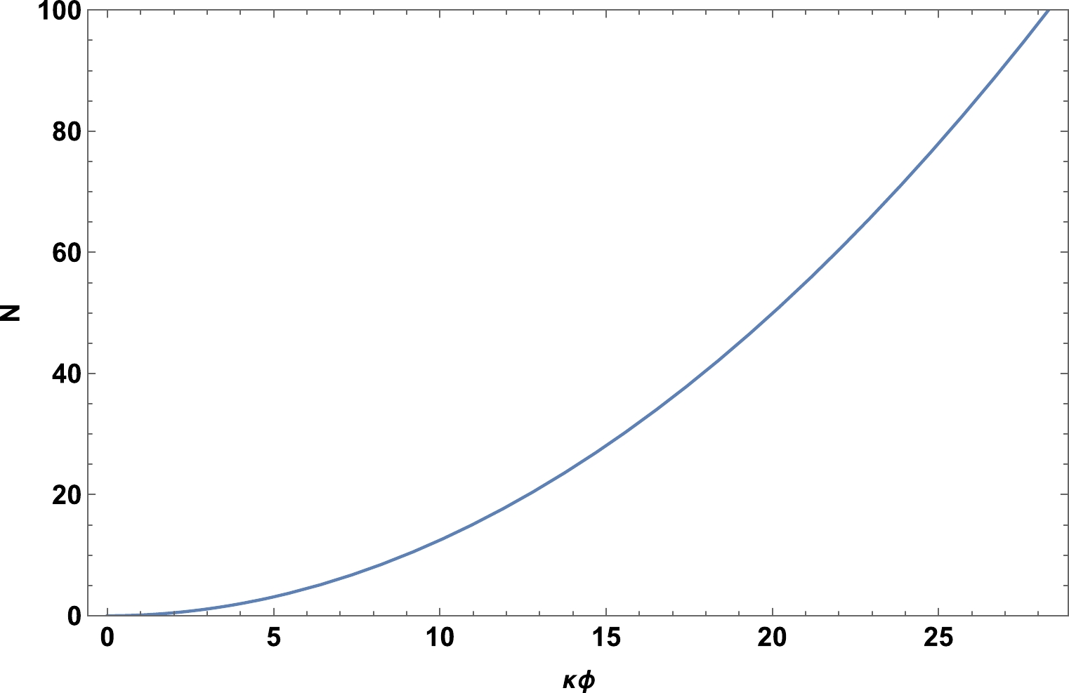

Figure 1

Figure 1.  (color online) Plot of the number of e-folds versus the scalar field ϕ for $\xi=10^{-3.5}$ and $\lambda=0.13.$

DownLoad: Full-Size Img PowerPoint

The slow roll parameter defined in Eq. (32) becomes

Figure 2 represents the evolution of the correction term $C_1$ as a function of the coupling constant ξ. Note that the effect of the Palatini parameter ω on $C_1$begins from an approximate value of $10^{-4}$. Note also that, for $\xi=0$, the correction term reduces to one, and the standard expression of the slow roll parameter is recovered. For $\xi\neq0$ and $\omega=0$, we recover the slow roll parameter expression in the case of NMC within the metric approach.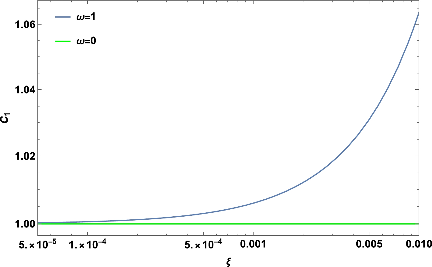

Figure 2

Figure 2.  (color online) Variation of the correction term $C_1$ as a function of the coupling constant for $N=45$.

DownLoad: Full-Size Img PowerPoint

The spectral index of the power spectrum given by Eq. (43) can be expressed as

Figures 3(a) and 3(b) illustrate the variation of $n_s$ against the number of e-folds N and against the scalar field for $N=45$, respectively, for $\lambda=0.13$ and for different values of the coupling constant ξ, i.e., $10^{-3.5}, 10^{-4}, 0,$ and $-10^{-4}$. The gray horizontal bound in both figures represents the limits for the spectral index imposed by Planck data. We conclude that the predictions of $n_s$ are consistent with the observational data for $\xi=10^{-4}$ and $\xi=10^{-3.5}$.

Figure 3

Figure 3.  (color online) Evolution of $n_s$ against the number of e-folds (a) and against the scalar field (b) for different values of the coupling constant ξ and $\lambda=0.13$.

DownLoad: Full-Size Img PowerPoint

From Eqs. (46) and (49), we can obtain the power spectrum of the amplitudes of the curvature and tensor perturbations as

respectively.

The behavior of $C_2$ is shown in Fig. 4. We present this term versus the coupling constant ξ in the cases of the hybrid Palatini metric formalism (blue curve) and metric formalism (green curve). The effect of the Palatini parameter ω on $A^2_s$ emerges from $\xi=5\times10^{-3}$.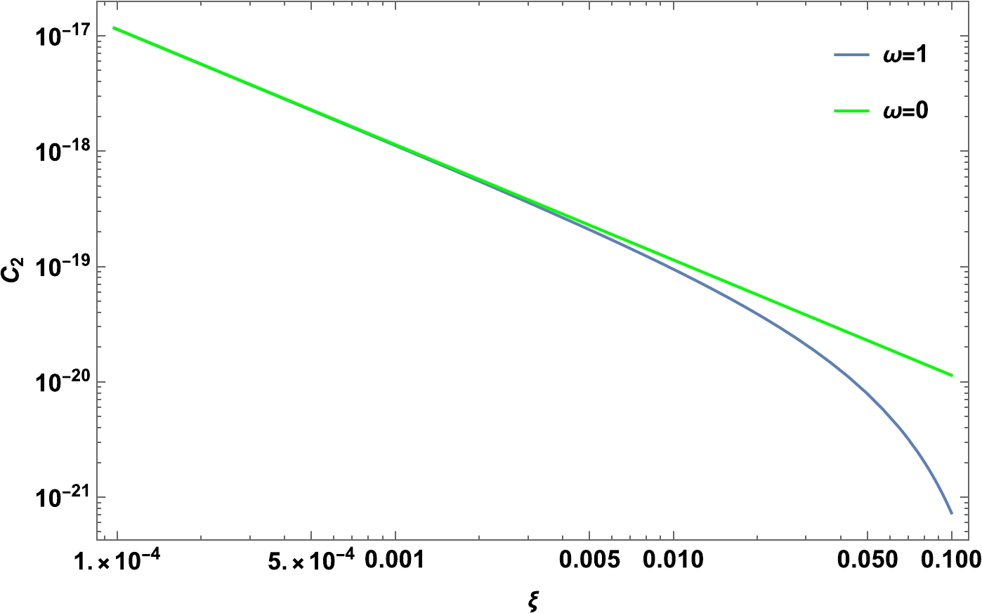

Figure 4

Figure 4.  (color online) Variation of the correction term $C_2$ versus the coupling constant for a number of e-folds $N=45$.

DownLoad: Full-Size Img PowerPoint

The correction term $C_3$ is plotted as a function of ξ in Fig. 5. Note that the effect of the Palatini parameter emerges from a value of $\xi= 10^{-2}$.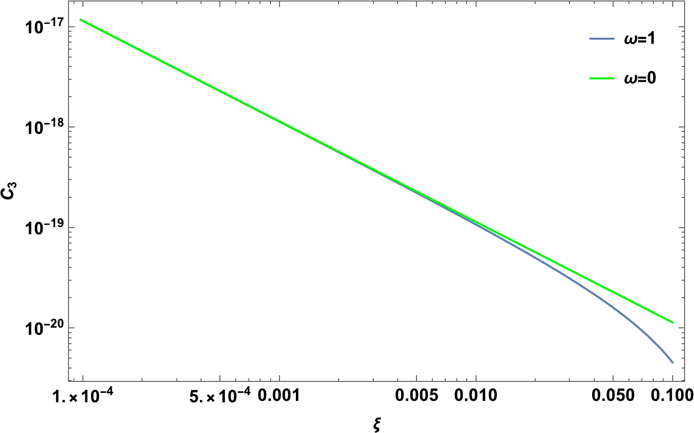

Figure 5

Figure 5.  (color online) Variation of the correction term $C_3$ against the coupling constant for a number of e-folds $N=45$.

DownLoad: Full-Size Img PowerPoint

From Eq. (51), the tensor to scalar ratio can be obtained as

Figure 6 shows the evolution of r versus the number of e-folds N for $\lambda=0.13$ and for selected values of the coupling constant ξ. Note that r lies within the bounds imposed by observational data [17] in the appropriate range of N for the selected values of ξ.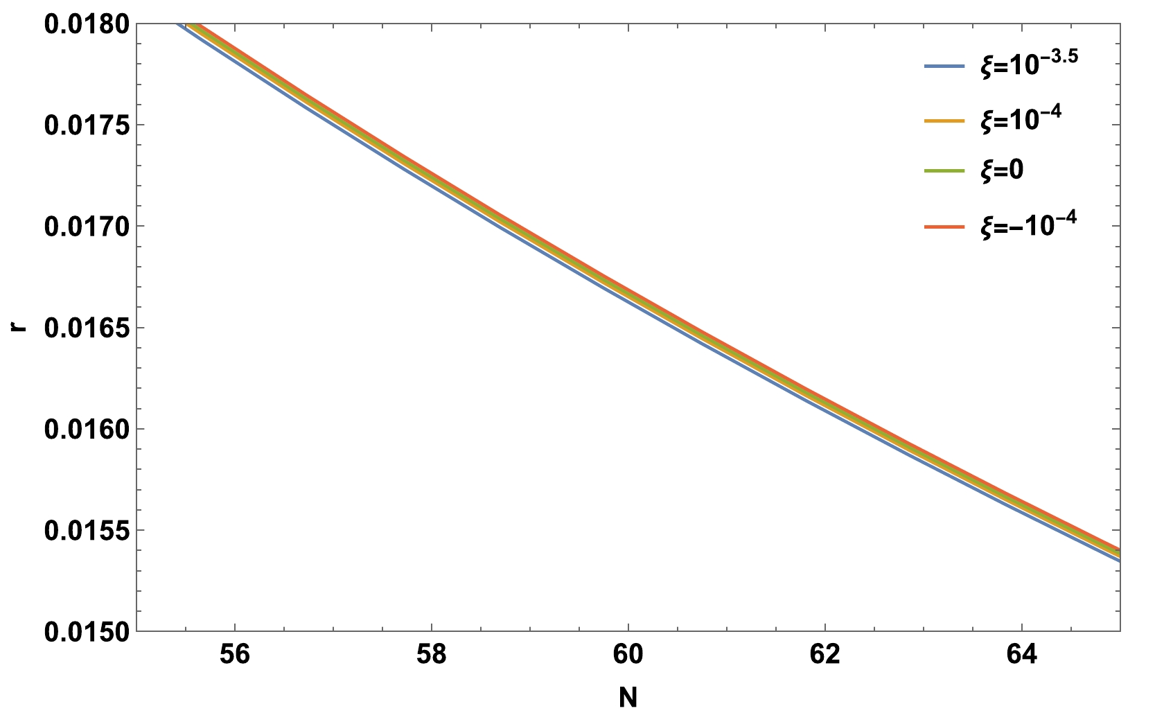

Figure 6

Figure 6.  (color online) Variation of the tensor to scalar ratio r as a function of the number of e-folds N for different values of the coupling constant.

DownLoad: Full-Size Img PowerPoint

Figure 7 shows the $(n_s, r)$ plane for different values of the coupling constant ξ in the range of the number of e-folds $30 \leq N \leq 90$ with the constraints from the Planck TT, TE, EE+LowE+lensing (gray contour) as well as Planck TT, TE, EE+lowE+lensing+BK14 data (red contour). Note also that $n_s-r$ predictions for the case where $\xi\leq 0$ are ruled out at $95\%$ confidence level contour according to the current observational data [17]. Furthermore, for $\xi=10^{-3.5}$, observational parameters lie within $68\%$ CL contour for a range of the number of e-folds $40.9\leq N\leq 47$ (low-N scenario). In addition, we obtain the central value of the index spectral $n_s=0.9649$ with a small value of tensor to scalar ratio $r=0.022$ for $N=43.43$. For $\xi=10^{-4}$, the results are inside the $68\%$ CL contour for the range $67.8\leq N \leq 86$ (high-N scenario). However, $N=75.41$ gives $n_s=0.9649$ and $r=0.013$. Thus, we can conclude that NMC in the framework of hybrid metric Palatini can ensure successful Higgs inflation. In the literature, it was reported that NMC in the Pure Palatini formalism requires a large value of ξ and results in an extremely small value of tensor to scalar ratio $r\sim 10^{-12}$ [54−56]. Therefore, the hybrid model may be an effective approach to solve this issue by increasing the value of r, making it comparable with the corresponding values predicted by the original metric approach. Then, it may be probed by future experiments [57, 58] where the value of the tensor to scalar ratio is on the order of $r\sim 10^{-2}$.

Figure 7

Figure 7.  (color online) Variation of the tensor to scalar ratio r against the scalar spectral index $n_s$ for selected values of the coupling constant. The gray and red contours correspond to the Planck TT, TE, EE+LowE+lensing and Planck TT, TE, EE+lowE+lensing+BK14 data, respectively.

DownLoad: Full-Size Img PowerPoint

VII. CONCLUSIONS

• I. INTRODUCTION
• II. SETUP
• III. SLOW ROLL EQUATIONS
• IV. SCALAR PERTURBATIONS
• V. TENSOR PERTURBATIONS
• VI. HIGGS INFLATION
• VII. CONCLUSIONS

In this study, we investigated a cosmological model where the field is non-minimally coupled with gravity in the hybrid metric Palatini approach.

We also analyzed the cosmological perturbations to determine the different parameters during the inflationary period. As previously mentioned, the existence of correction terms to the standard background and perturbative parameters represents the impact of the Palatini approach and the non-minimal coupling between the scalar field and the Ricci scalar.

We applied our model by comprehensively developing a non-minimally coupled inflationary model driven by the Higgs field with a quartic potential within the slow-roll approximation.

We checked our results by plotting the evolution of different inflationary parameters versus the constraints provided by the observational data.

We found that perturbed parameters such as the tensor to scalar ratio and the scalar spectral index are compatible with the observational data for an appropriate range of the number of e-folds for different values of ξ, as shown in Figs. 3 and 6.

We plotted the different correction terms to the standard case versus the coupling constant. We showed that they depend on NMC and the Palatini effect.

Finally, for further checking the consistency of our model, we compared our theoretical predictions with observational data [17] by plotting the Planck confidence contours in the plane of $n_{s}-r$ (Fig. 6). The results show that the predicted parameters are in good agreement with the Planck data for two values of the NMC constant: $\xi=10^{-3.5}$ and $\xi=10^{-4}$.

1Hybrid metric Palatini Higgs inflation was also considered in [33] using the Einstein-frame analysis. The framework considered by the authors of this paper, however, is completely based on a non minimal coupling between the Higgs field and both the metric and the Palatini Ricci scalar curvature. Whereas, in our analysis, non minimal coupling is between the Higgs field and the Palatini scalar curvature alone.

References