


 Abstract
 HTML
HTML Reference
 Related
 PDF
PDF


-
The Sun is considered a high-energy astrophysical source owing to its interactions with cosmic rays. Cosmic-ray electrons undergo inverse-Compton scattering with sunlight and produce a diffused gamma-ray halo around the Sun [1−3]. Synchrotron radiation from the electrons produces a disk emission from radio to X-rays [4]. Moreover, cosmic-ray nuclei interact with the solar atmosphere hadronically and produce secondary gamma rays and neutrinos [5−7]. The latter component is mainly emitted from the photosphere and is thus more concentrated than the inverse-Compton halo. We refer to it as solar disk emission.
The solar disk gamma-ray emission was first detected with EGRET [8, 9] and later with Fermi-LAT with much better precision [10]. The observed emission is higher than early estimates by almost an order of magnitude [6]. Subsequent analyses with six years [11] and nine years of Fermi data [12, 13] have found several new features, including the following: 1) the flux anticorrelates with solar activity at low energies (~ 1 GeV) and at the highest detected energy (~ 100 GeV) with a much larger correlation amplitude, 2) the flux exhibits a hard spectral index (
$ \sim E^{-2.2} $ ) and reaches up to at least 200 GeV during solar minimum, 3) a spectral dip is observed around 30–50 GeV, and 4) the photon distribution on the projected Sun disk (solar gamma-ray morphology) varies strongly as a function of the solar cycle. See Ref. [14] for a brief overview and Ref. [15] for the latest solar gamma-ray observation covering the full solar cycle. Currently, no theoretical model or calculation can completely explain these observational features.The
$ >100 $ GeV gamma-ray emission, in particular, is highly variable; six photons were observed in 1.4 years near the solar minimum but none in the 7.8 years afterward [12]. The solar minimum spectrum is also much harder than the cosmic-ray spectrum. These suggest that very-high-energy observation of the Sun is another valuable avenue for probing the underlying physics. Only large ground-based air-shower array experiments, such as ARGO-YBJ, HAWC, and LHAASO can observe the Sun at TeV energies. ARGO-YBJ has provided the first set of strong constraints on sub-TeV to 10 TeV emission during the quiet Sun period from 2008–2010 [16]. HAWC provided a stronger constraint [17] using data from November 2014 to December 2017. Recently, HAWC has detected TeV gamma rays with a soft spectrum with six years of data [18]. The Sun was more active in that period; therefore, the high-energy spectrum is expected to be soft from Fermi observations. IceCube has performed the first dedicated search of solar atmospheric neutrinos [19], but the sensitivity is still above the predicted flux [20, 21].The first detailed computation of the solar disk gamma-ray flux was performed by Seckel, Stanev, and Gaisser [6], who proposed that charged cosmic rays entering the atmosphere are reflected by concentrated magnetic flux tubes and thus enhance the gamma-ray production compared to the zero-magnetic field case. Most subsequent calculations on gamma rays [22, 23] and neutrinos [7, 20, 21] have ignored magnetic fields. In Ref. [22], the minimum disk emission from the Sun limb was estimated with zero-magnetic field calculations, and in Ref. [12], the maximum was estimated by assuming all cosmic rays are reflected on the solar surface and produce gamma rays with 100% efficiency. Most recently, Refs. [24] and [25] have considered the effect of magnetic fields around the Sun in the context of solar gamma-ray production. However, none of the calculations can explain the observations, such as the flux, spectral shape, and time variability.
In this study, we investigate solar disk emission production using the particle simulation toolkit
$\mathrm{Geant4}$ , along with the observation-based PFSS magnetic-field model, to better understand the phenomenologies behind cosmic rays interacting with the Sun. -
$\mathrm{Geant4}$ is a software toolkit that simulates the passage of particles through matter [26]. Due to its powerful functionality and modeling capability,${\mathrm{Geant4}}$ is used in many applications, such as high-energy physics, nuclear physics, medical science, and space science. We base our computation on version$\mathrm{10.3.3}$ .A typical
$\mathrm{Geant4}$ simulation contains many components, such as detector designation, event generator, particle definition, and physics models. We focused on particles within the energy range between 100 MeV and 100 TeV, which covers the energy range of Fermi and HAWC. Following the user's guide [27] and the Geant4 recommendation for high energy physics (HEP), we use the FTFP-BERT physics list to model both hadronic and electromagnetic interactions. Below 5 GeV, the Bertini cascade model [28] is used. The Fritiof string model is used above 4 GeV, with a transition between 4−5 GeV [29]. When simulating particle propagation, we set the simulation procedure to stop and kill particles below 100 MeV. Thus, the main physical processes during particle tracking are hadronic decay, electron/positron bremsstrahlung, and annihilation.Magnetic fields are included in
$\mathrm{Geant4}$ through a separate class. In order to propagate a particle inside a magnetic field, Geant4 solves the Lorentz force equation of motion of the particle. Geant4 breaks up this curved path into linear chord segments to calculate the track's motion in a field. Following the$\mathrm{Geant4}$ guide, we compute the particle tracks using the default Runge-Kutta method. We also adopted Geant4’s default stepper, “ClassicalRK4,” and set the chord segment to 10 m.We have enabled the standard physics lists with Geant4 for hadronic and electromagnetic interactions, except synchrotron radiation. However, the solar photon is not included. Thus, the simulation does not include synchrotron and inverse Compton energy losses. Generally, given the short distance scales of the problem, these processes are subdominant compared to hadronic and electromagnetic interactions in the matter, except perhaps at much higher energies than our problem at hand [30] or maybe at longer distance scales [4].
-
Based on the
${\mathrm{Geant4}}$ toolkit, we developed$\mathrm{G4SOLAR}$ , a program that handles particle propagation and particle interactions in the solar atmosphere. In this section, we describe the essential components of$\mathrm{G4SOLAR}$ . -
The atmosphere of the Sun consists of the photosphere, chromosphere, and corona [31]. The photosphere, with an approximate thickness of 500 km, is the layer where the Sun becomes optically opaque. The chromosphere is the region roughly a few thousand km above the photosphere, and the corona is defined as the large region above the chromosphere, where the temperature rises to millions of kelvin.
Figure 1 shows the density distribution of the solar atmosphere used in our calculation. Below the photosphere (set at 0 km), we use the density provided by Ref. [32], and we use Eq. (2.1) of Ref. [6] to extend it to 1600 km. Between 1600 and 3000 km, we use the data in Ref. [33]. We configure the Sun as a sphere and divide the region from –600 km to +3000 km into 3600 equal-thickness layers following the density profile shown in the figure.
-
For magnetic fields near the Sun, we consider the potential field source surface (PFSS) model [34−37], which describes the large-scale magnetic fields above the photosphere,
$ R_{\odot} $ . Using the photospheric magnetic-field measurement as a boundary condition and assuming that the current density is zero and the fields are completely radial at a distance,$ R_{ss}\sim {\cal O}(1)R_{\odot} $ , the magnetic fields between$ R_{\odot} $ and$ R_{ss} $ can be computed by solving for the scalar potential. Thus, for each complete Carrington cycle ($ \sim27 $ days), using the photospheric measurements by observatories such as GONG [38] and SOHO/MDI [39], a PFSS model can be obtained with only$ R_{ss} $ as a free parameter, which is fitted separately. Notably, the large-scale magnetic fields we consider differ drastically from the small-scale magnetic flux tube used by Seckel et al. [6]; we compare with their results in detail in Sec. III.H. The PFSS model is easy to implement and was found to agree reasonably well with more detailed and computationally expensive magnetohydrodynamic models [40], thus making it a natural choice for our simulation study.The PFSS models are obtained using the Solar Software (SSW) package [41]. We consider the Carrington Rotations 2070(CR2070) (13 May 2008 to 9 Jun 2008) for solar minimum and 2149(CR2149) (07 Apr 2014 to 04 May 2014) for solar maximum. In the PFSS model, we use spherical harmonic coefficients with order 9 to calculate magnetic fields. The source surface parameter is chosen to be 1.6
$ R_{\odot} $ for solar minimum and 2.5$ R_{\odot} $ for solar maximum. Hereafter, we denote the solar minimum case as$\mathrm{Quiet}$ , the solar maximum case as$\mathrm{Active}$ , and the control case with a zero magnetic field as$\mathrm{NoField}$ . The magnetic field we obtained by PFSS for both$\mathrm{Quiet}$ and$\mathrm{Active}$ are visualized in Fig. 2. For the$\mathrm{Quiet}$ case, the$ B_r $ is mainly distributed in two poles, and the overall magnetic field strength is smaller than the$\mathrm{Active}$ case. For the$\mathrm{Active}$ case, Br is mainly distributed near the equator.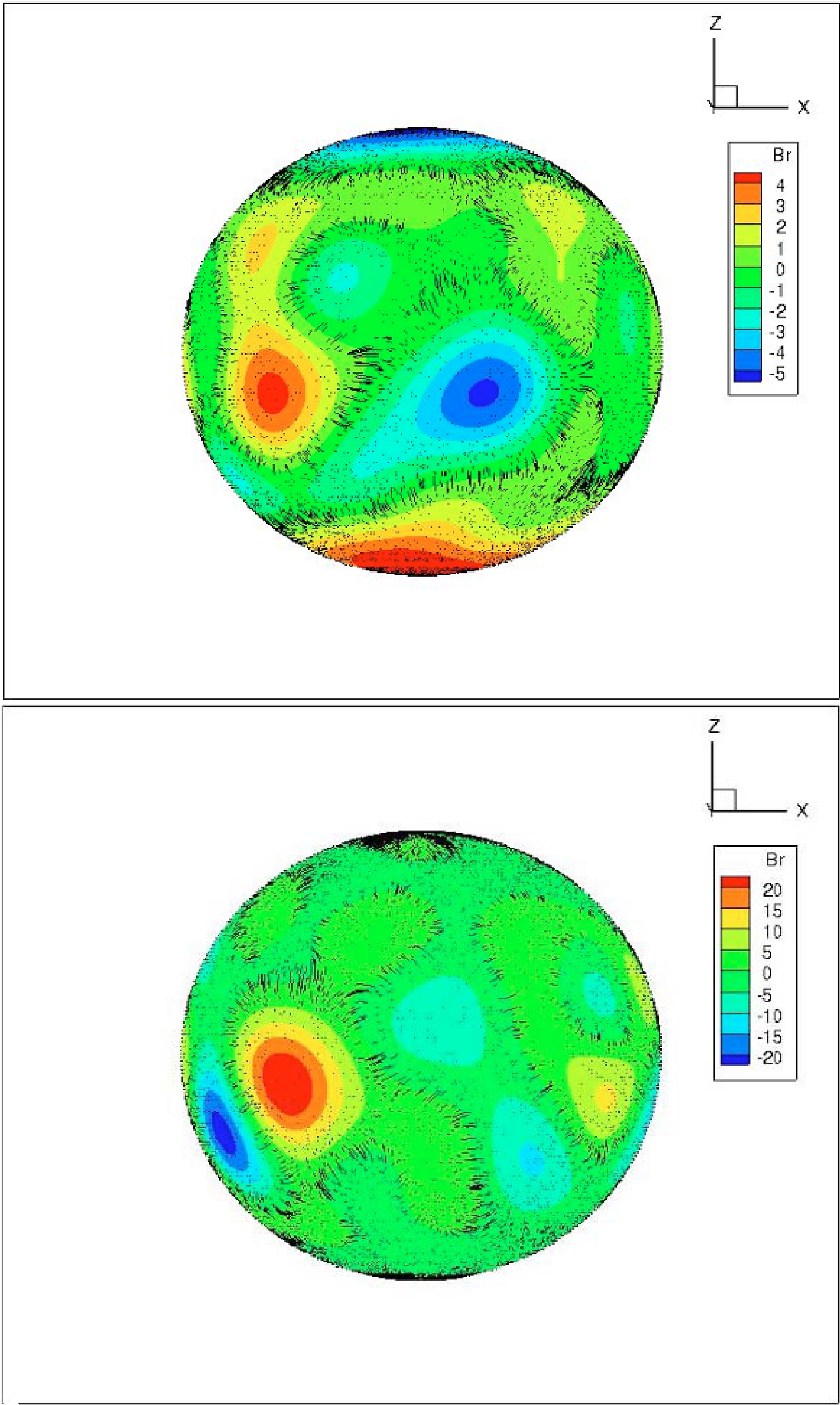
Figure 2. (color online) Obtained magnetic field distribution in the spherical coordinates for both
$\mathrm{Quiet}$ (above) and$\mathrm{Active}$ (below) for CR2070 and CR2149, respectively. The color-bar for$ B_r $ is in the Gauss unit. The black lines indicate the magnetic field line structure at a solar radius close to the photosphere surface. The dipole structure in the$\mathrm{Quiet}$ case can be clearly seen. The field strength in the$\mathrm{Active}$ case is stronger overall, and the dipole structure becomes unclear.We evaluate the PFSS model in a 361 (radial)
$ \times $ 180 (polar)$ \times $ 360 (azimuthal) grid in our simulation volume. This resolution means that we neglect small-scale magnetic field variations below roughly$ 10^{4} $ km in the tangential direction. We note that typically, the PFSS model starts at the photosphere. For our purpose, we extrapolate the PFSS model down to 600 km below the photosphere by setting the fields to be the same as those at the surface. Because we start our simulation at +3000 km, we practically ignore all the magnetic fields above this height. During simulation, the value of the magnetic fields at each point in the simulation volume is then obtained by interpolating these grid points. In this work, we have neglected the magnetic field variation below the resolution of the magnetic field grid points [42]. These resolutions are limited by computation power and, ultimately, by the PFSS model itself. These field variations could affect the propagation of low energy particles with a Larmor radius below the grid size (about$ 10^4 $ km in the tangential direction and 10km in the radial direction). We leave the modeling of sub-grid effects for future work.Table 1 and Fig. 3 show the mean values of the magnetic fields and their standard deviations for the two phases of solar activity with the PFSS model. We obtain the mean and the deviation values by sampling 100,000 points randomly at the photosphere. These values are stable versus height. Changing the sampling point between –600 km and +3000 km changes the values by a few percent. In general, the mean values are close to zero due to averaging regions with magnetic fields in opposite directions. The standard deviation is thus more representative of the typical field strength of the model, which is
$ \simeq 2 $ G for the$\mathrm{Quiet}$ case. However, the standard deviation is much larger for the$\mathrm{Active}$ case,$ \simeq 15 $ G for the r and θ components.$<B_{r}> [G] $ 

$<B_{\theta}> [G] $ 

$<B_{\phi}> [G] $ 

$\mathrm{Quiet}$ 

0.03 $ \pm $ 2.16

0.11 $ \pm $ 2.22

−1.04 $ \pm $ 2.45

$\mathrm{Active}$ 

−0.35 $ \pm $ 15.42

0.66 $ \pm $ 15.46

0.77 $ \pm $ 2.54

Table 1. Mean values for the three components of the PFSS magnetic fields and their standard deviations for the
$\mathrm{Quiet}$ and$\mathrm{Active}$ cases evaluated at the photosphere.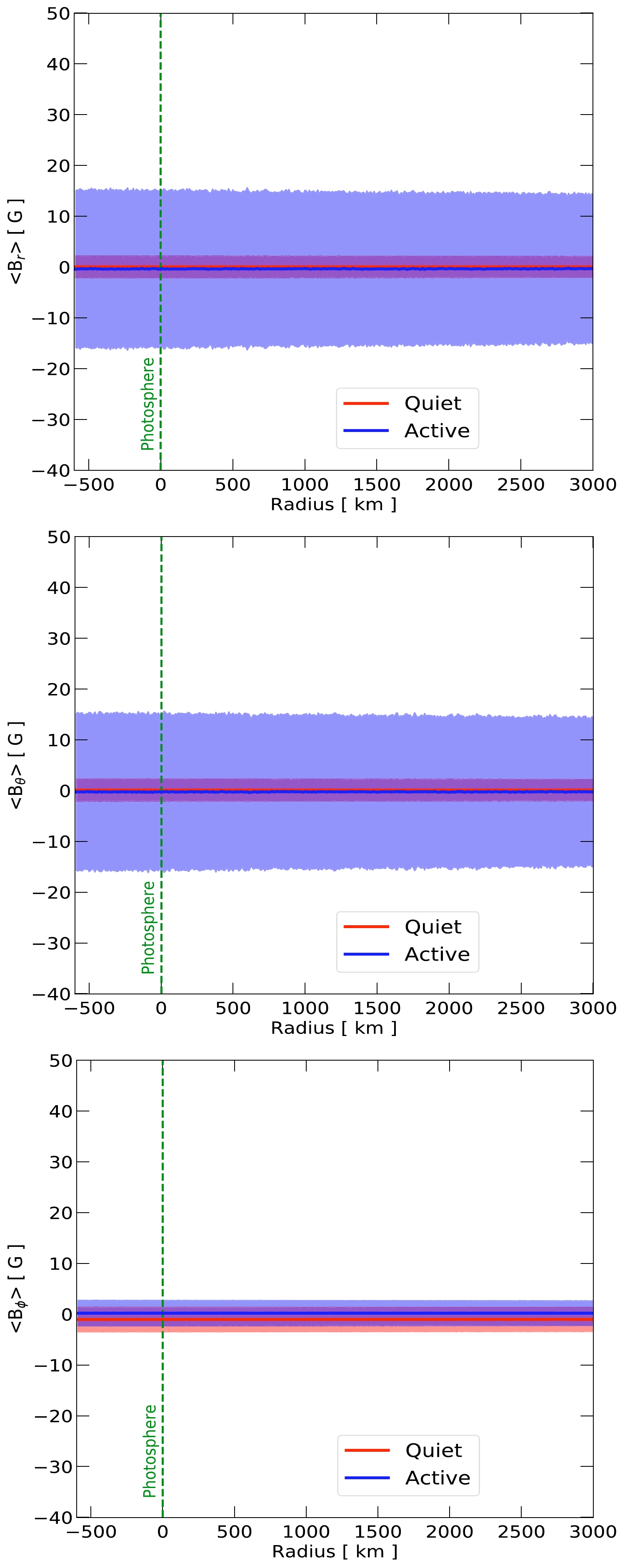
Figure 3. (color online) From top to bottom, the figures showcase the average magnetic field components B
$ _r $ , B$ _{\theta} $ , and B$ _{\phi} $ at distances of 600 km below and 3000 km above the photosphere. Above our simulation volume at 3000 km, the field strength is set to be zero. The solid lines and shaded bands indicate the average values and deviations, respectively. "Quiet" represents the solar minimum of CR2070, and "Active" represents the solar maximum of CR2149. -
The final component of
$\mathrm{G4SOLAR}$ is the position and direction sampling of the cosmic-ray particles. The starting positions of the input particles are first sampled uniformly at 3000 km above the photosphere. We consider the energy between 100 MeV and 100 TeV, which is divided uniformly into six logarithmic intervals. For each interval, the energy is sampled with a spectral index -1 (uniform in log.), and the sampling size varies owing to computational time considerations, with the number of particles between$ 10^5 $ and$ 10^6 $ .The momentum vectors of the particles at the input position also need to be sampled. We define the incident angle,
$ \omega_{p} $ , as the angle between the momentum vector and the normal direction of the spherical simulation volume at particle position (see Sec. III.E). The number of particles is then sampled according to$N \propto \sin\omega_{p} \cos\omega_{p}$ . Here,$ \sin\omega_{p} $ is the solid angle factor, and$ \cos\omega_{p} $ considers the geometric factor between the incoming cosmic-ray flux and the receiving surface element. The azimuthal directions of the particles are sampled uniformly. In our setup, only events with$ \omega_{p} \geq 90^\circ $ can enter and interact with the Sun. Thus, we only sample in the range between$ 90^{\circ} $ and$ 180^{\circ} $ .All the particles are tracked only when they are in the simulation volume. Thus, for particles leaving the –600 km layer, we assume they are completely absorbed, and for particles leaving the 3000 km layer, we assume they have escaped. The simulation results thus consist of all the escaped gamma-ray events.
-
Connecting the simulation results to real world situations requires the cosmic-ray spectrum. It is well-known that the Sun can change the cosmic-ray propagation environment in the solar system [43] and modulate the cosmic-ray flux as the rays propagate inward from interstellar space. It is thus natural to expect that additional modulations exist when cosmic rays propagate from the Earth's orbit to the vicinity of the Sun. However, cosmic-ray propagation in the solar system is still an open problem [44], likely important only at low energies. For simplicity, we use the cosmic-ray spectrum measured at the Earth's position as our default result. Solar modulation suppresses low-energy cosmic rays; thus, it could suppress the actual gamma-ray production compared to our default results. We discuss and further investigate the effect of solar modulations in Sec. III.F.
We set the composition of the Sun to be 100% protons and only consider cosmic-ray protons. Including heavier species, such as helium, in both cosmic rays and the atmosphere could enhance gamma-ray production. We discuss this and estimate the effect in Sec. III.I.
We use the 2006 proton spectrum by
$\mathrm{PAMELA}$ [45] from 0.1 GeV to 45 GeV, then$\mathrm{AMS-02}$ [46] from 45 GeV to 2.5 TeV, and finally$\mathrm{CREAM}$ [47] up to 100 TeV.All the photon events leaving the simulation volume are collected and re-weighted to account for the cosmic-ray spectrum and normalized to obtain the photon luminosity per unit area (at the injection radius) per unit time. The photon flux at the Earth is then obtained by considering the scaling factor
$ (R_{\odot} + 3000\,{\rm km})^2/{\rm AU}^2 $ . The γ-ray flux at the Earth,$ F_{\gamma,\oplus} $ , is obtained by converting the simulated production yield,$ F_{\gamma,\oplus}=\frac{{\rm d}N_{\gamma,mc}}{{\rm d}E_{\gamma}{\rm d}S{\rm d}t} \cdot \frac{F_{p,\odot}}{F_{mc}} \cdot \frac{(R_{\odot} + 3000\,{\rm km})^2}{{\rm AU}^2} \, , $

(1) where
${\rm d}N_{\gamma,mc}/{\rm d}E_{\gamma}{\rm d}S{\rm d}t$ is the normalized γ-ray yield (event per energy per area per time) obtained at the$ R_\odot $ +3000 km surface,$ F_{p,\odot} $ is the proton spectrum from observation, and$ F_{mc} $ is the proton spectrum we put in the simulation. -
We first consider the
$\mathrm{NoField}$ case to cross check and validate the simulation procedure. The simulation and analysis are performed without magnetic fields; otherwise all procedures are identical to the cases with magnetic fields.Figure 4 shows the results for the
$\mathrm{NoField}$ case. We compare them with the semi-analytic calculation by Zhou et al. [22], where they assumed that the incoming cosmic rays and the gamma rays produced are collinear. With this approximation, only cosmic rays pointed at the Earth and grazing through the edge of the solar atmosphere can produce detectable gamma rays (Sun limb). This limb flux can be easily calculated as it is a 1D computation; the resultant flux roughly follows the cosmic-ray spectral index. We find that our$\mathrm{NoField}$ results agree well with Zhou et al. above 10 GeV, meaning that the collinear approximation is appropriate here. Below 10 GeV, the$\mathrm{NoField}$ case has much higher gamma-ray production due to large-angle gamma-ray events. We discuss this in more detail in Sec. III.E.1. Above a few TeV, we start to see deviations due to the imposed cosmic-ray energy cutoff at 100 TeV.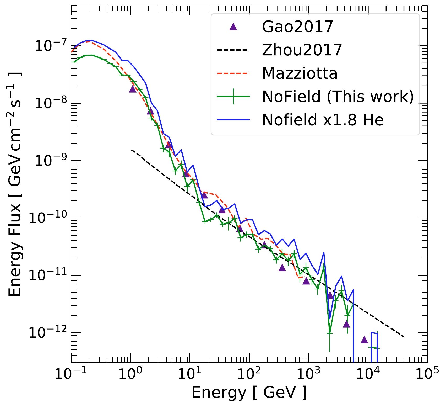
Figure 4. (color online) Simulated solar disk gamma-ray flux without magnetic fields (
$\mathrm{NoField}$ ). For comparison, we also show the 1D semi-analytic calculation by Zhou et al. [22], simplified$\mathrm{Geant4}$ simulation result by Gao et al. [23], and simulation result with FLUKA by Mazziotta et al. [24]. The blue solid line is our result but scaled with the nuclei effects. (See Sec. III.I) The enhanced gamma-ray production below 10 GeV is due to large-angle events caused by kinematics. See Sec. III.E.1 for details.We then compare our results with Gao et al. [23], the precursor of this work, where the cosmic-ray position sampling step was not implemented owing to the spherical symmetry of the problem when magnetic fields are not included. We find that our results agree well with each other. This validates our 3D position and angle sampling procedures described in Sec. II.A, which are necessary once global solar magnetic fields are introduced.
We also compare our
$\mathrm{NoField}$ results with those of Mazziotta et al. [24], which performed essentially the same calculation but with the FLUKA simulation package. Considering the contribution due to nuclei effects (see Sec. III.I), our results are in excellent agreement with each other, up to some fluctuations due to simulation. -
Figure 5 shows the solar disk gamma-ray flux for
$\mathrm{Quiet}$ and$\mathrm{Active}$ together with that for$\mathrm{NoField}$ . We find that the PFSS magnetic fields can dramatically change gamma-ray production. At 100 MeV, all three cases have similar flux (see Sec. III.E.2 for further discussion). Between 100 MeV and 10 GeV, the$\mathrm{Quiet}$ and$\mathrm{Active}$ cases exhibit harder spectral shapes and have a higher flux than the$\mathrm{NoField}$ case. The difference in flux is the largest at approximately 10 GeV, by almost two orders of magnitude. Above 10 GeV, the spectra fall sharply and have spectral shapes even softer than the cosmic-ray spectrum. At approximately 1 TeV, the$\mathrm{Quiet}$ flux and$\mathrm{Active}$ fluxes merge with the$\mathrm{NoField}$ flux, showing that the PFSS magnetic fields can no longer affect the gamma-ray production. We interpret these observations using the event angular distributions in Sec. III.E.2.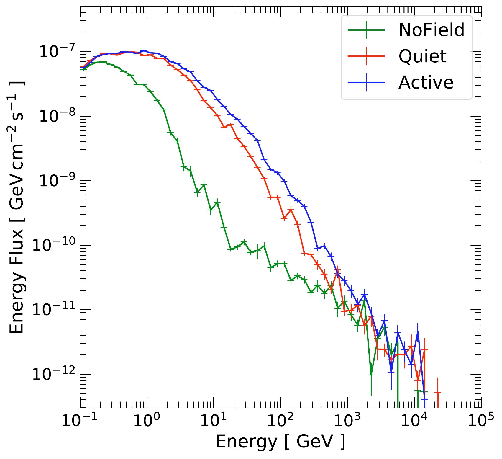
Figure 5. (color online) Solar disk gamma-ray flux computed by
$\mathrm{G4SOLAR}$ without magnetic fields ($\mathrm{NoField}$ ), with solar minimum PFSS magnetic fields ($\mathrm{Quiet}$ ), and with solar maximum PFSS magnetic fields ($\mathrm{Active}$ ). The magnetic fields boost gamma-ray production by enhancing the production of large-angle events. See Sec. III.E.2 for details.Comparing the results between
$\mathrm{Quiet}$ and$\mathrm{Active}$ , the two fluxes have similar shapes, except that the$\mathrm{Active}$ flux becomes larger by about a factor of two between 1 GeV and 1 TeV.In the next few subsections, we explore the simulation results in detail and attempt to understand the various properties of these results.
-
Figure 6 shows the breakdown of the physical processes that contribute to the solar disk gamma-ray production. For all three cases, we find that the dominant contribution comes from neutral pion (
$ \pi^{0} $ ) decays. These pions could be produced directly from the primary proton interactions or from the subsequent hadronic showers. Due to the short lifetime of$ \pi^{0} $ , they decay promptly before undergoing additional scatterings. As a result,$ \pi^{0} $ can efficiently convert the primary proton energy into gamma rays.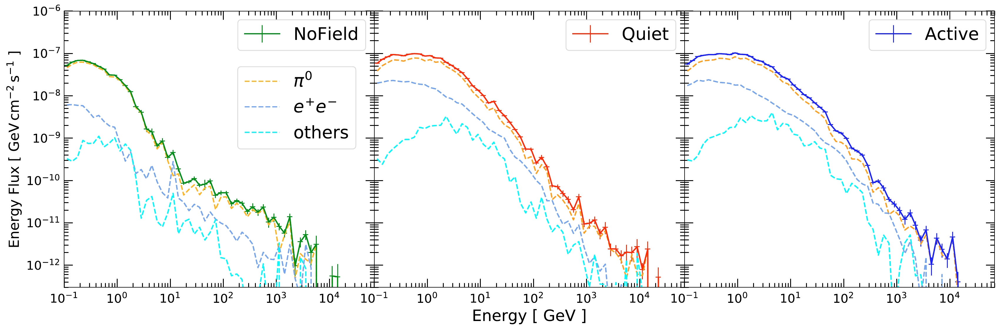
Figure 6. (color online) Breakdown of the total flux into the physical processes responsible for gamma-ray production. The dominant process is neutral pion decay, followed by electron/positron bremsstrahlung and annihilation, and finally, miscellaneous processes, including the decay of heavier hadron states. See the text for details.
The second most important source of gamma rays, at the ~ 10% level, comes from electron and positron bremsstrahlung as well as positron annihilation (labeled simply as
$ e^{+}e^{-} $ ). These electrons and positrons come from the final states of many secondaries (e.g.,$ \pi^{\pm} $ ) or can be produced from electromagnetic showers initiated by energetic gamma rays or electrons.Finally, we group the remaining gamma-ray production channels into "others," which include the decay of heavier hadron states (e.g.,
$ \eta, \Sigma, \Omega $ , etc.), hadron inelastic scatterings, and muon-bremsstrahlung. These contributions are subdominant but not negligible. -
Figure 7 shows the contributions from each input proton energy interval to the total gamma-ray flux. Interestingly, for proton energies ranging from 0.1 GeV to 10 GeV, we find no significant changes in the contribution between
$\mathrm{NoField}$ and those with magnetic fields. Most of the flux enhancements for$\mathrm{Quiet}$ and$\mathrm{Active}$ come from proton energies from 10 GeV to 1 TeV, where the low energy "tails" in the$\mathrm{NoField}$ case change into "bumps" in the cases with magnetic fields. While gamma-ray production is enhanced from 1 TeV to 100 TeV, the enhancements are mainly at low energies, buried by the other low-proton-energy components, and have little effect on the final results.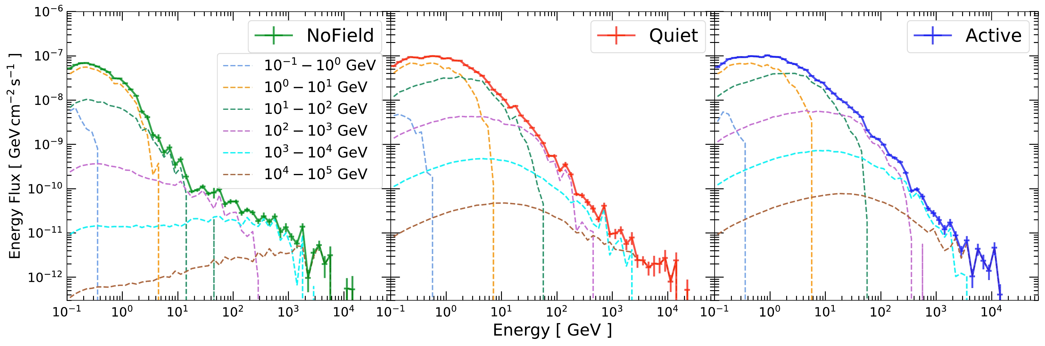
Figure 7. (color online) Breakdown of the total flux into the contributions from the corresponding input proton energy intervals. Vertical lines correspond to isolated nonzero energy bins.
-
We explore in detail the angular distributions of protons interacting in the solar atmosphere and those of the outgoing gamma rays, which we find helpful in elucidating the physics behind the enhanced gamma-ray production with magnetic fields. We consider three angles,
$ \omega_{p} $ ,$ \omega_{\gamma} $ , and$ \omega_{\gamma p} $ , which are illustrated schematically in Fig. 8.
Figure 8. (color online) The definitions of the angles considered in Sec.III.E. Schematically, the gray region highlights the simulation volume. The black arrow is the normal direction from the center of the Sun, and the dark red (blue) arrow is the proton (gamma-ray) velocity vector.
Figure 9 shows the angular distribution of the outgoing gamma rays. We define the angle
$ \omega_{\gamma} $ as the angle between the vector of the escaped gamma rays and the normal direction of the spherical simulation volume, evaluated at +3000 km above the photosphere. In other words,$ \cos(\omega_{\gamma}) $ = 1, 0 correspond to gamma rays pointing radially outward and tangential to the simulation volume, respectively.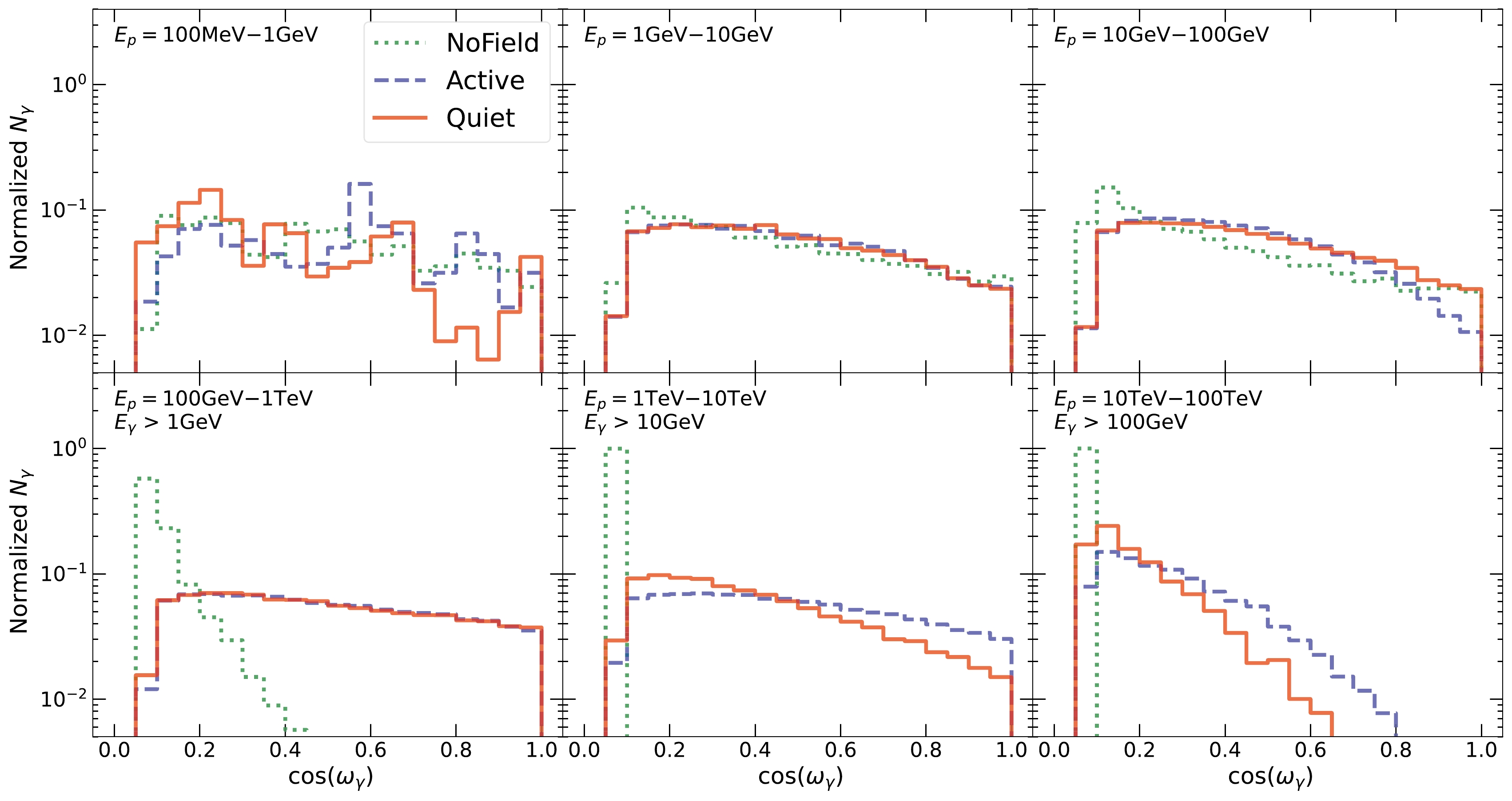
Figure 9. (color online) Angular distribution of the gamma rays produced in
$\mathrm{NoField}$ ,$\mathrm{Quiet}$ , and$\mathrm{Active}$ .$ \cos(\omega_{\gamma}) = 1 $ corresponds to the radially outward direction, and$ \cos(\omega_{\gamma}) = 0 $ corresponds to the tangential direction. Each panel corresponds to an interval of the input proton energies, and the distributions are all renormalized to have the same area. For display purposes, gamma-ray energy cuts are applied in the bottom three panels. At high energies, all three distributions peak at$ \cos(\omega_{\gamma}) \simeq 0 $ , which corresponds to the Sun-limb scenario [22]. However, the cases with magnetic fields have broader distributions at all energies, especially at medium energies. These large-angle contributions are responsible for the enhanced solar gamma-ray production compared to the$\mathrm{NoField}$ case. Notably, the$\mathrm{NoField}$ distribution is also broadened at low energies (with the gamma-ray flux enhanced), likely due to kinematic effects.Similarly, Fig. 10 shows the angular distribution for the incoming protons, where the angle
$ \omega_{p} $ is defined by the angle between the proton vector and the normal direction at +3000 km. Here, we only consider protons that have successfully produced at least one escaped photon; protons that are completely absorbed or escaped without producing gamma rays are not included.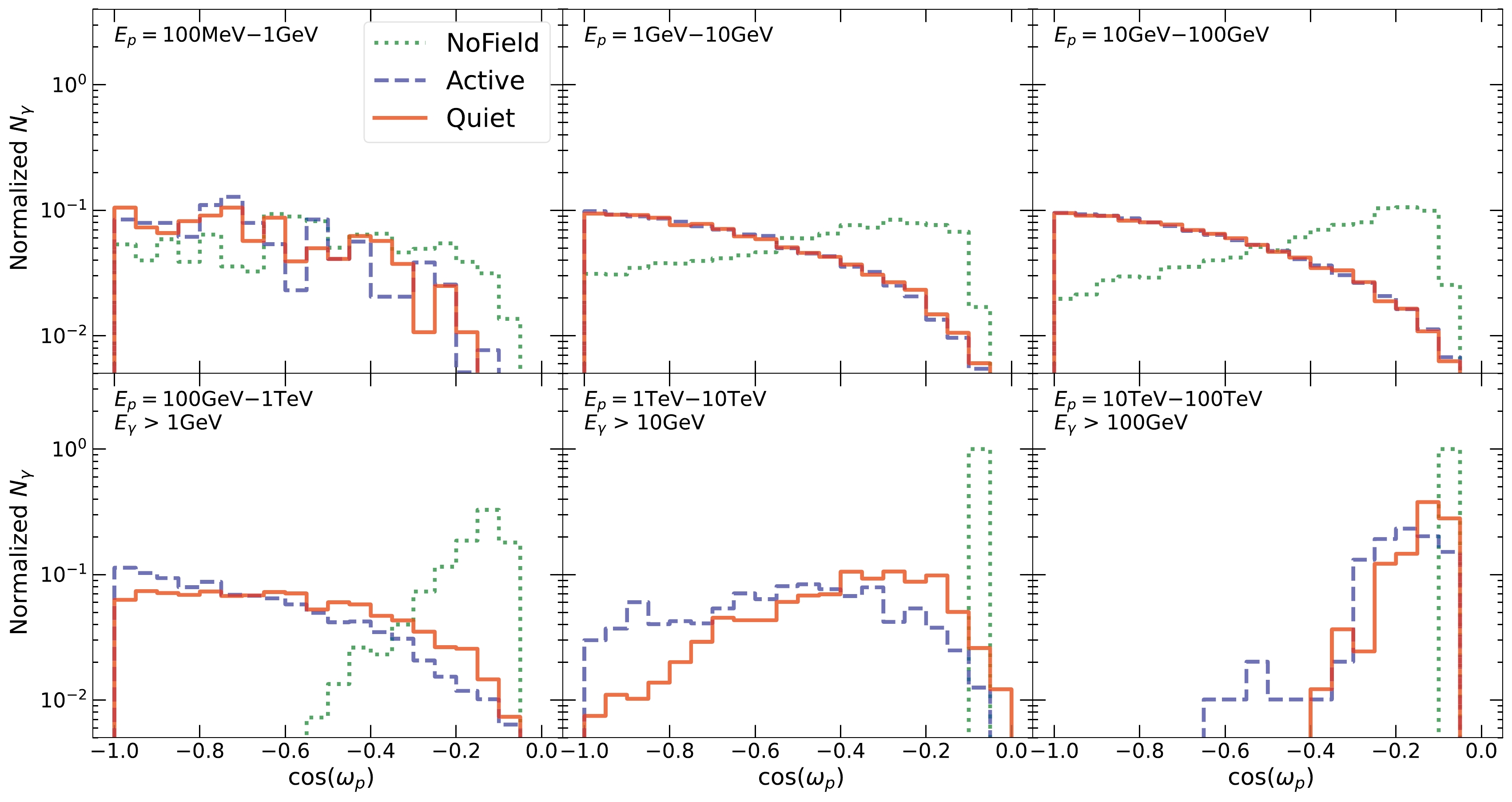
Figure 10. (color online) Similar to Fig. 9 but for the angular distribution of the incoming protons that have successfully produced an outgoing photon.
$ \omega_{p} $ is defined as the angle between the incoming proton vector and the normal direction of the simulation volume at the proton injection position. Therefore,$ \cos{\omega_{p}} \simeq 0 $ corresponds to the Sun-limb scenario. The inclusion of magnetic fields broadens the angular distributions, which are responsible for the enhanced gamma-ray production. Note that the higher$\mathrm{Active}$ flux compared to the$\mathrm{Quiet}$ flux from$ E_{p} > $ 100 GeV (Fig. 7) is reflected here by the broader angular distributions.Finally, Fig. 11 shows the distribution for
$ \omega_{\gamma p} $ , defined as the angles between the outgoing gamma rays and the incoming protons that produce gamma rays. Each proton could contribute multiple outgoing photons; all these pairs are considered in the distribution.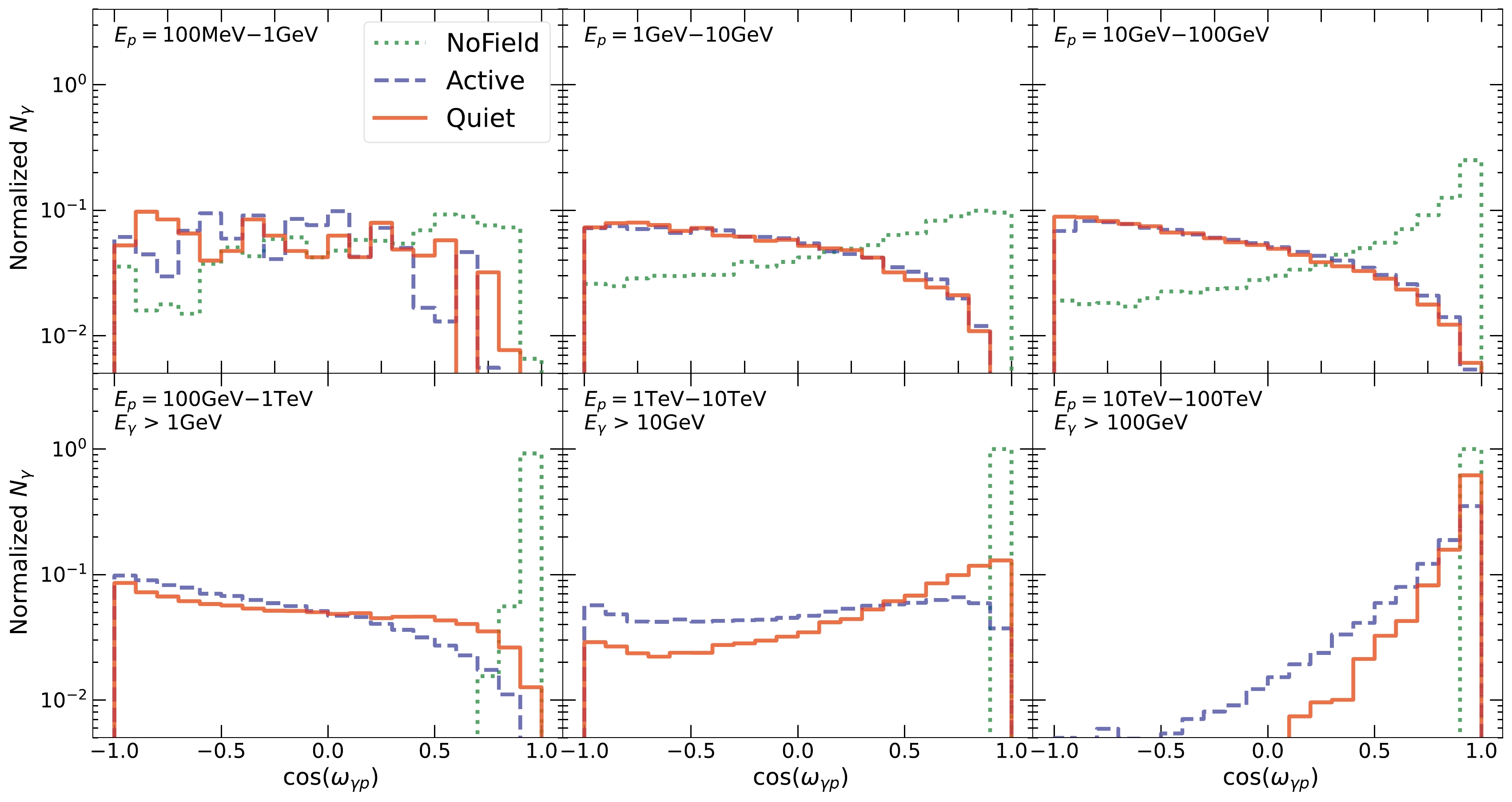
Figure 11. (color online) Similar to Fig. 9 but for the angular distribution between each pair of incoming protons and outgoing gamma rays,
$ \omega_{\gamma p} $ . At high energies, the peaked distributions correspond to the outgoing gamma rays having nearly the same direction as the incoming protons, which reflects the high Lorentz factor effect. Considering Fig. 10 and Fig. 9 reaffirms that this is the Sun-limb scenario. The introduction of magnetic fields evidently broadens this distribution, enhancing gamma-ray production. In addition, the distribution for the$\mathrm{NoField}$ case is also broad at low energies, likely due to kinematic effects. This is responsible for the enhanced$\mathrm{NoField}$ flux compared to the flux in the limb case. We also note that all three cases have similarly broad angular distributions at the lowest energy bin, showing that the enhancement saturates, as shown in the lowest energy bins in Fig. 7.We note that for high proton energies, many lower-energy gamma rays are produced, which are not important to the problem at hand, as shown in Sec. III.D. Therefore, to highlight the angular distribution for the relevant photons, we apply gamma-ray energy cuts
$ E_{\gamma}>1 $ GeV,$ E_{\gamma}>10 $ GeV, and$ E_{\gamma}>100 $ GeV for the three proton energy intervals above 100 GeV, respectively. -
It is instructive to first consider the
$\mathrm{NoField}$ case. At high energies ($ E_{p}>100 $ GeV), we find that the distributions tend towards$ \omega_{\gamma}\simeq 90^{\circ} $ ,$ \omega_{p}\simeq 90^{\circ} $ , and$ \omega_{\gamma p }\simeq 0^{\circ} $ . This peaked angular distribution appears naturally due to the large Lorentz factor (except for the low-energy secondary photons that are cut from the figures). This corresponds to the Sun-limb scenarios, as discussed in Ref. [22].However, for lower energy protons with energy less than roughly 100 GeV, we find that the distribution becomes significantly broader. Because there are no magnetic fields to change the trajectories of the particles, the broader distribution must be due to the scattering angular distribution itself. This is expected to be caused by large transverse momentum distribution for the pion produced after scattering [48, 49].
The broader angular distribution can also explain the difference between the calculations by Zhou et al. [22] and the simulation results from this work and Gao et al. [23]. With the 1D approximation used by Zhou et al., gamma rays produced by protons with steep incident angles are all absorbed. However, as shown in our 3D calculation, e.g., the
$ \omega_{p} $ distribution of 1−100 GeV, the distribution is broad, and even down-going protons ($ \omega_{p}\sim 180^{\circ} $ ) can produce observable gamma rays. This is also precisely the proton energy range responsible for the enhanced gamma-ray flux ($ E_{\gamma}\sim 1 $ GeV) in our simulation compared to that by Zhou et al. Therefore, we conclude that, by kinematic effects alone, proton-proton scattering can produce large-angle events responsible for enhancing gamma-ray production around 1 GeV. At higher energies, as gamma rays and protons become more collinear, the 3D and 1D calculations produce similar results. -
Comparing the angular distributions of
$\mathrm{NoField}$ with that from$\mathrm{Quiet}$ and$\mathrm{Active}$ , we see that the PFSS magnetic fields significantly impact the distribution. This is expected as both the directions of the primary protons and the charged secondaries ($ \pi^{\pm} $ ,$ e^{\pm} $ , etc.) are bent as they propagate in the simulation volume. The bending effect is evidently shown in the$ \omega_{p} $ distribution. Importantly, as the$\mathrm{NoField}$ distribution becomes more peaked for$ E_{p}>100 $ GeV, the distribution with magnetic fields remains broad until$ E_{p}>10 $ TeV. Following the observations from the previous section, the broader distribution is responsible for the enhanced gamma-ray production compared with the$\mathrm{NoField}$ case. We conclude that the broadening of the angular distributions due to magnetic fields bending the cosmic-ray primaries and secondaries can enhance the solar gamma-ray production.We note that our results with and without magnetic fields all have roughly the same flux at 100 MeV. We believe this is somewhat accidental. On the one hand, the magnetic fields broaden the angular distribution and enhance gamma-ray flux production. On the other hand, magnetic fields can also deflect the cosmic rays and reduce the overall production rate. This calculation may not fully reflect the latter effect, as we consider consider a propagation space of 3000 km above the photosphere. We leave a more thorough investigation of this for future works.
Finally, comparing between the
$\mathrm{Quiet}$ and$\mathrm{Active}$ results, we find that the$\mathrm{Active}$ angular distribution has more large-angle contributions than that for$\mathrm{Quiet}$ . This also explains why our simulation results find that the$\mathrm{Active}$ flux is larger than the$\mathrm{Quiet}$ flux around 10 GeV−1 TeV. This follows from Table 1, where$\mathrm{Active}$ has typically higher magnetic fields than$\mathrm{Quiet}$ , thus leading to more magnetic bendings. On the other hand, the$\mathrm{Quiet}$ result is similar to the$\mathrm{Active}$ result around 1 GeV. This suggests that below 1 GeV, larger magnetic fields do not further enhance gamma-ray production, which is also shown by the similar$ \omega_{\gamma p} $ distribution for proton energies between 1 GeV and 100 GeV. In other words, the magnetic-field enhancement effect saturates. -
It is instructive to estimate the gyroradius, which puts the length and energy scales into perspective. The shortest length scale of our simulation is in the radial direction, 3600 km. Setting this as the gyroradius and considering 10 G as a typical field strength (Sec. II.B.2), the critical energy is
$ E_{c} \simeq {\rm 1 TeV} \left( \frac{r}{3600\,{\rm km}} \right) \left( \frac{B}{10\,{\rm G}} \right) \, . $

(2) This means that protons with energies below
$ E_{c} $ could undergo a complete reversal in their pointing direction in the simulation volume. Above$ E_{c} $ , one would then expect the effect of magnetic fields to decrease and approach the collinear limit. Indeed, this is consistent with observations from Figs. 10 and 11, showing that the angular distributions undergo a qualitative change below and above TeV. -
We have considered a fixed cosmic-ray spectrum measured at the Earth for the incoming cosmic rays, ignoring the effect of solar modulation and additional modulation from the Earth to the Sun. The latter, in particular, has substantial theoretical uncertainties.
To estimate the effect of solar modulation, we use the simple yet effective force field approach [43]. We follow Ref. [10] to compute the cosmic-ray spectrum near the solar surface. The local interstellar spectrum,
$ F_{lis}(E) $ , is taken from Ref. [50]. The cosmic-ray spectrum at different solar radii is then given by$ F_{p}(E,r)= F_{lis}(E) \frac{E^{2} - m_{p}^{2}c^{4}}{ \left(E+\Phi(r) \right)^{2} -m_{p}^{2}c^{4} }\, , $

(3) where
$ \Phi(r) $ is the modulation potential. We adopt the modulation potentials that are first derived in Ref. [2] based on the results from Ref. [51]. Two modulation potentials are considered. Model-1, suitable for solar cycles 20/22, is given as$ \begin{array}{*{20}{l}} \Phi_1(r)= \dfrac{\Phi_0}{1.88}\left\{ \begin{array}{ll} r^{-0.4} - r_b^{-0.4}, & r\ge r_0,\\ 0.24 + 8 (r^{-0.1} - r_0^{-0.1}), & r<r_0 \end{array} \right. \end{array} $

(4) and Model-2, suitable for solar cycle 21, is
$ \begin{array}{*{20}{l}} \Phi_2(r)= \Phi_0 (r^{-0.1} - r_b^{-0.1}) / (1 - r_b^{-0.1}). \end{array} $

(5) Here,
$ \Phi_0 $ is the modulation potential at 1 AU,$ r_{0} = 10 $ AU, and$ r_{b} = 100 $ AU (we note that Model-3 in Ref. [10] assumes no additional solar modulation inside the Earth radius, which corresponds to our default assumption).Our default results (as in Fig. 5) correspond to having a force field potential at Earth position,
$ \Phi_{0} $ , to be around 600 MV. To estimate the effect of modulation, we consider$ \Phi_{0}=300 $ MV and$ \Phi_{0}=1000 $ MV for solar minimum and solar maximum, respectively. We re-weigh our simulation result using these modulated spectra and obtain the corresponding output gamma-ray flux. Notably, the models and the parameters chosen here do not correspond to the same periods as the measured Fermi data. Thus, this only served as a qualitative estimate of the effect of solar modulation.Figure 12 shows the modulated gamma-ray flux. The red (blue) band shows the
$\mathrm{Quiet}$ ($\mathrm{Active}$ ) case, where the solar minimum (maximum) force field potential is used. The upper edge of the band corresponds to Model-2, and the lower edge corresponds to Model-1.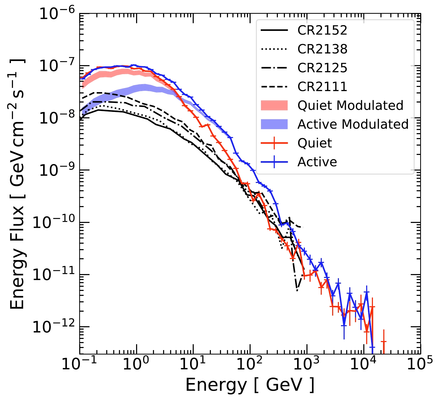
Figure 12. (color online) The bands show the effect of considering solar modulation on solar gamma-ray production. The upper edge of the band corresponds to Model-2 from Ref. [10], while the lower edge corresponds to Model-1. The force field potential for the modulated
$\mathrm{Quiet}$ ($\mathrm{Active}$ ) case is chosen to be 300 (1000) MV. For comparison, the un-modulated results from Fig. 5 are also shown. As shown, solar modulation could affect the final gamma-ray flux substantially at low energy but negligibly for gamma rays above 10 GeV. Simulation results, including the four magnetic field models CR2152, CR2138, CR2125, and CR2111 from Ref. [24], are also displayed. A detailed comparison is provided in Sec.III.H.As expected, the effect of solar modulation is mostly at low energies, with stronger suppression at lower energies. Due to the modulation, the
$\mathrm{Active}$ flux is now lower than the$\mathrm{Quiet}$ flux below a few GeV. Qualitatively, the solar modulation effect could be responsible for some and possibly all of the time variation seen in the low-energy Fermi data [13, 15]. We leave a detailed time-variation comparison with data for future works.Notably, the effect of solar modulation diminishes above 10 GeV. Therefore, the large time variation seen above 100 GeV [12, 13] cannot be solely explained by the cosmic-ray solar modulation models. This, yet again, provides evidence that other magnetic structures are needed to explain these events. It is also quite possible that they could affect the production of low-energy gamma-ray events.
-
Figure 13 shows our simulated solar disk emission together with observational results and constraints. Results with solar modulation are shown in colored bands, and those without solar modulation are shown in solar lines with error bars corresponding to uncertainties due to Monte Carlo simulations. The green solid line corresponds to the case without considering any magnetic fields. For observation results, we show the
$ \simeq $ 1.5-year result (Aug. 2008 – Feb. 2010) obtained by the Fermi collaboration [10] and the$ \simeq $ 1.5-year result (Aug. 2008 – Jan. 2010) obtained by Tang et al. [13] that extended the analysis to higher energy. During these periods, the Sun is dominantly in quiet states, which we simply denote as solar minimum. We also show the 9-year analysis (Aug. 2008 – Jul. 2017) by Tang et al. covering both low and high solar activity periods.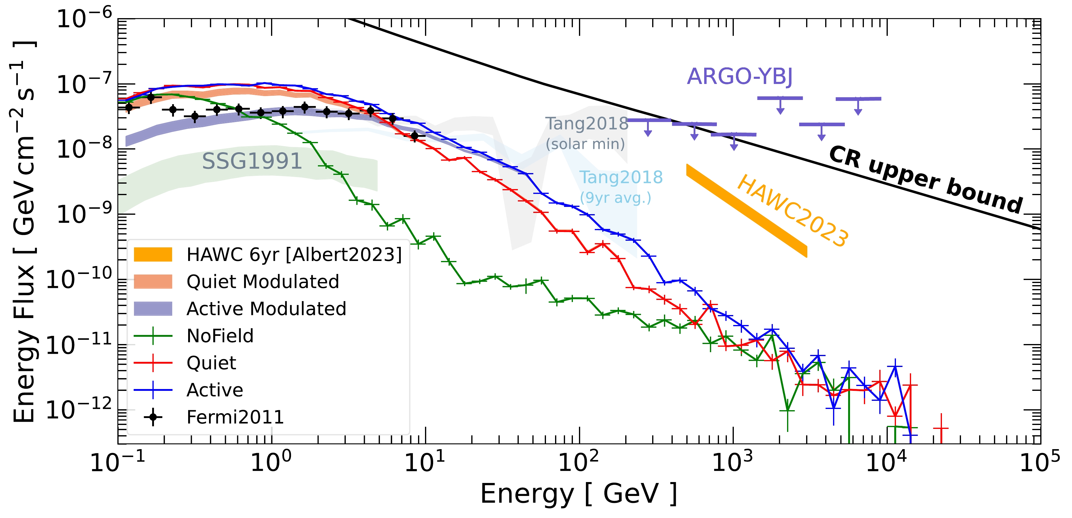
Figure 13. (color online) Our simulation results (
$\mathrm{NoField}$ ,$\mathrm{Quiet}$ ,$\mathrm{Active}$ , Quiet Modulated, and Active Modulated) compared with solar disk observations from the 1.5-year analysis by the Fermi collaboration [10], follow-up analysis with a similar period by Tang et al. [13], and their 9-year averaged results. The comparison of the model with the Fermi-LAT data refers to different time intervals. The solar minimum case of Fermi-LAT is from 2008-8-7 to 2010-1-21, while the “Quiet” case in our model refers to a solar magnetic configuration before the launch of the Fermi satellite from 2008-5-9 to 2008-6-9. The simulated gamma-ray spectrum affected by solar modulation for the maximum and minimum activity models is also displayed. We also show the prediction from Seckel et al. [6] (SSG1991) and the theoretical upper bound from Linden et al. [12]. The upper limits at high energies come from ARGO-YBJ [16] and detection by HAWC [18].At low energies, between 0.1 GeV and 10 GeV, our results with magnetic fields are comparable to the solar minimum flux up to a factor of a few. Interestingly, the Fermi observation suggests that the flux at this energy range anti-correlates with solar activities [11, 13]. This is consistent with our results with solar modulation. In short, PFSS magnetic fields with solar modulation could qualitatively explain the low-energy Fermi data. However, as explained below, this picture may not be complete due to the discrepancy at high energies.
At higher energies, our results fall below the data quickly. At 100 GeV, both the
$\mathrm{Quiet}$ and$\mathrm{Active}$ results are approximately one order of magnitude less than the observation. In particular, the spectrum of the solar minimum observation was found to be hard until at least 200 GeV with no signs of cutoff, making the disagreement with our results even larger. For the 9-year averaged spectrum, which is dominated by periods of higher solar activity, the spectrum softens rapidly above 100 GeV and could potentially align with our calculations. However, the measurement quality is not sufficient to draw conclusive statements yet. Lastly, we also do not see the extreme time variability for the$ >100 $ GeV photon flux and the spectral dip around 30−50 GeV [12, 13]. Thus, new magnetic fields or new physics ingredients are required, in addition to coronal fields, to explain the high-energy photon flux. Approximately 1 TeV cosmic rays are needed to produce 100 GeV photons; therefore, modulating cosmic rays alone cannot explain the extreme time variability observed at 100 GeV.Above the Fermi-LAT energy range, only large ground-based air shower gamma-ray observatories can potentially detect high-energy gamma rays from the Sun. We show the upper limits from ARGO-YBJ [52] and the detection by HAWC [18], both of which are orders of magnitude higher than our calculation. For reference, we also show the theoretical upper limit from cosmic rays interacting with the atmosphere [12]. Given that the solar minimum flux measurement by Fermi did not exhibit a cutoff, a detection could be possible with HAWC or LHAASO. TeV detection or constraint will be essential for identifying the mechanism responsible for the high-energy flux.
-
For many years, the only solar disk gamma-ray calculation that took into account magnetic fields was the pioneer work by Seckel, Stanev, and Gaisser (SSG1991 [6]). In SSG1991, cosmic-ray propagation in the solar system was considered, and more importantly, cosmic rays entering the solar atmosphere were assumed to be funneled into magnetic flux tubes and then reflected in the flux tubes due to the large field gradient. As a result, the gamma-ray production is enhanced by the possibility of cosmic rays interacting after being reflected. However, despite such an enhancement, the SSG1991 model prediction is still much lower than the observation. Interestingly, in this work, we find that at low energies, scattering kinematics and coronal magnetic fields can provide more than enough boost to gamma-ray production. Thus, we find that the SSG1991 flux-tube reflection may be a subdominant mechanism for enhancing gamma-ray production. However, flux tubes could still be important for bringing the 0.1–10 GeV flux to quantitatively match the observational data.
Compared to existing solar gamma-ray calculations with magnetic fields, Mazziotta et al. [24] have independently published a work that used another particle interaction simulation package,
$\mathrm{FLUKA}$ [53] to simulate the solar disk gamma-ray production with PFSS magnetic fields. Compared to our results, Mazziotta et al. considered cosmic-ray propagation in the solar system using a custom propagation code called HelioProp instead of the force field model; they also employed a larger simulation volume filled with the PFSS magnetic fields. They consider the PFSS fields from four Carrington rotations from 2011 to 2014, roughly in the middle between a solar minimum and maximum. Despite all the differences, our results agree with Mazziotta et al. qualitatively in the sense that with PFSS magnetic fields, the$ \sim 1 $ GeV gamma-ray production is boosted to close to the level of Fermi data. Quantitatively, our results are a factor of a few higher than Mazziotta et al. when comparing more similar solar activity periods. This difference could be due to differences in the chosen simulation volume, magnetic field resolution, and solar modulation models. Our results reach good agreement with each other, approximately above 100 GeV. Mazziotta et al. also showed that gamma-ray production at higher energies can be further enhanced with an enhanced magnetic field profile near the photosphere (the$\mathrm{BIFROST}$ profile). This is in good agreement with our physical interpretation of the nature of the boost mechanism in Sec.III.E.2. However, with or without the boosted magnetic field profile, the Fermi gamma-ray data above 100 GeV during solar minimum still cannot be explained. This agrees with our conclusion that coronal magnetic fields can not explain the high-energy disk emission.In the study by Hudson et al. [25], an overview of the solar surface magnetic field configuration from inside the convection zone to the corona was provided in the context of charged particle propagation. This includes both cosmic rays and energetic particles accelerated by the Sun. The discussion mostly focused on lower energy particles that follow the field lines closely, e.g., as in Ref. [54, 55]. Nevertheless, the magnetic field structure discussed in this work will likely be an important addition to fully calculating solar particle propagation in the Sun.
-
We have only considered protons in cosmic rays and the solar atmosphere. Adding the nuclei species would slightly enhance the gamma-ray production. This is often taken into account by considering the so-called nuclear enhancement factor. Following Ref. [56], we compute the enhancement factor due to p-He, He-p, and He-He interactions. Considering the He/p number abundance ratio in the photosphere to be about 8% [57] and the He/p ratio in the cosmic rays to be about 8%−10%, the combined enhancement factor due to helium increases the gamma-ray flux production by about a factor of 1.6 to 1.8. The effects from other species are substantially smaller.
The effect of nuclear species, though not exactly tiny, is subdominant to uncertainties associated with the complicated solar magnetic fields. Also, this small factor does not change our conclusions. Thus, we leave the full implementation of nuclear effects to future works.
-
In this study, we present our
$\mathrm{Geant4}$ based code,$\mathrm{G4SOLAR}$ , which simulates cosmic-ray interactions with magnetic fields in the solar atmosphere. Using$\mathrm{G4SOLAR}$ , we compute the solar disk gamma-ray flux in three: scenarios without magnetic fields ($\mathrm{NoField}$ ), with coronal magnetic fields during low solar activity ($\mathrm{Quiet}$ ), and with magnetic fields during peak solar activity ($\mathrm{Active}$ ). We use the PFSS coronal magnetic field model and only focus on the volume from 600 km below the photosphere to 3000 km above, where interactions are expected to happen. It is clear that the inclusion of magnetic fields enhances gamma-ray production compared to the$\mathrm{NoField}$ case [25].From the simulated gamma-ray flux spectrum and by studying their underlying composition and angular distributions, we have these main findings:
● Without magnetic fields, the solar disk flux production below 10 GeV can be significantly enhanced due to photons produced with large scattering angles relative to the primary proton direction purely due to particle scattering kinematics.
● With the PFSS magnetic fields, the solar disk flux production is further enhanced up to 1 TeV. This is due to a much wider angular distribution for the escaped gamma rays caused by magnetic fields bending the trajectories of primary protons and charged secondaries.
While significant quantitative disagreements exist between our result and the observations [10−13], we believe this work has elucidated at least one pathway that could lead to a complete model for explaining the solar disk gamma-ray flux.
-
In this study, we find that coronal fields cannot explain the observed gamma rays above 100 GeV, especially during solar minimum. This suggests that features with stronger magnetic fields, e.g., sunspots or active regions, could be responsible for producing high-energy gamma rays. However, this contradicts the observed time variation [12, 13], where more high-energy photons were observed from the Sun during solar minimum when the sunspots are few. We leave these investigations for future works.
One of the main simplifications in our simulation is taking the simulation space boundary to be 3000 km above the photosphere. However, PFSS fields could affect the cosmic-ray propagation up to
$ {\cal O}(1) $ solar radii above the photosphere. Then, at a distance further than that, solar modulation of cosmic rays should be the dominant effect. Thus, in our setup, the effect of the PFSS magnetic fields could be underestimated at low energies. We leave further investigation of this for future works.Our results between 0.1 and 10 GeV seem to agree with the observed data up to a factor of a few. However, the data at approximately 100 GeV differs from the calculation by roughly an order of magnitude, suggesting that additional physics inputs are needed for qualitative explanations at high energies. Naturally, one would expect that strong magnetic field sources responsible for the high-energy gamma rays could also affect the production of low-energy gamma rays. Therefore, without a model for the whole energy range, we believe it is too early to state that PFSS fields and solar modulation are solely responsible for the ~GeV solar gamma-ray observation. However, PFSS fields certainly play an integral part in producing ~GeV solar gamma rays.
The gamma-ray data by Fermi-LAT [10−13] provide a rich set of phenomena that is neither mentioned nor explained in this work, including time variations, spectral features, and gamma-ray morphology. Furthermore, cosmic-ray Sun shadows [58−62] should be intimately related to the production of the disk gamma rays [63]. We anticipate that, once the relevant magnetic fields are identified or included in the calculation, these features and observations will be important for verifying or differentiating competing models.
In the very-high-energy regime, HAWC and LHAASO could provide valuable information for understanding the production of solar gamma rays. Recent results by HAWC [18] have shown that the Sun continues to emit gamma rays at the TeV energy range but with a much softer spectrum. LHAASO, with a larger collecting area, is expected to produce more precise measurements. It is clear from this work (also Ref. [24]) that PFSS magnetic fields could not account for the TeV solar emission. New magnetic-field structures or ideas, e.g., Ref [64], are needed to explain these TeV solar gamma-ray fluxes.
High-energy neutrinos are inevitably produced with the solar disk gamma-ray flux [5−7, 20, 21, 24, 65, 66] and could be detected by neutrino telescopes [19]. At the same time, the Sun is an important target for dark matter searches, where the signal could be anomalous neutrinos [67−74] and gamma rays [75−77]. Searches of these signals have yielded some of the strongest dark matter constraints in the literature [24, 78−82]. Having a robust model of cosmic rays interacting with the Sun is important for getting an accurate background estimate for these dark matter searches [20, 21, 83].
Ultimately, a precise understanding of how cosmic rays interact with the Sun could allow high-energy gamma rays and neutrinos to be new windows for probing solar magnetic fields [44, 84−89] and offer new perspectives in solar physics.
-
We thank John Beacom, Annika Peter, Tim Linden, Mehr Un Nisa, Bei Zhou, and Guanying Zhu for their helpful comments. We also acknowledge the essential support of Guofu Cao, Yiqing Guo, Shuangquan Liu, and Cong Li in developing the
$\mathrm{G4SOLAR}$ code.
Simulating gamma-ray production from cosmic rays interacting with the solar atmosphere in the presence of coronal magnetic fields
- Received Date: 2023-10-19
- Available Online: 2024-04-15
Abstract: Cosmic rays can interact with the solar atmosphere and produce a slew of secondary messengers, making the Sun a bright gamma-ray source in the sky. Detailed observations with Fermi-LAT have shown that these interactions must be strongly affected by solar magnetic fields in order to produce a wide range of observational features, such as a high flux and hard spectrum. However, the detailed mechanisms behind these features are still a mystery. In this study, we tackle this problem by performing particle-interaction simulations in the solar atmosphere in the presence of coronal magnetic fields using the potential field source surface (PFSS) model. We find that low-energy (~ GeV) gamma-ray production is significantly enhanced by the coronal magnetic fields, but the enhancement decreases rapidly with energy. The enhancement directly correlates with the production of gamma rays with large deviation angles relative to the input cosmic-ray direction. We conclude that coronal magnetic fields are essential for correctly modeling solar disk gamma rays below 10 GeV, but above that, the effect of coronal magnetic fields diminishes. Other magnetic field structures are needed to explain the high-energy disk emission.


 DownLoad: