


 Abstract
 HTML
HTML Reference
 Related
 PDF
PDF


-
The CNO cycle is a proton capture catalytic sequence that serves as the secondary mechanism for converting hydrogen into helium in the stellar environment [1, 2]. The hydrogen burning rate of the CNO cycle is significant for both nucleosynthesis and elemental production, as well as determining the lifetime of stars [3]. The 14N(p, γ)15O is the slowest reaction in the cycle, which determines the rate of energy production [4]. The continuous enrichment of 14N in the solar component is maintained based on the rate of 14N(p, γ)15O. Solar neutrino's spectral composition is also impacted by this reaction [5, 6]. Because of the shorter lifetime of 15O in comparison to 13N, the β decay of 15O is predicted to dominate the production of CNO neutrinos [7].
Numerous researchers [7−11] have examined the 14N(p, γ)15O cross-section for over 50 years. It was noted that only the measurements conducted by Schröder et al. [11] covered a broad energy range. It was also suggested that the
$ E1 $ transitions to the ground state ($ 1/2^{-} $ ) and$ M1 $ transitions to the 4th excited state ($ 3/2^{+} $ ) play a crucial role in the$ {\rm{S}}(0) $ measurements. Bertone et al. [12] measured the lifetime of$E_{x}$ =6.7931 MeV±1.7 keV state in 15O. Based on their new value for the lifetime of this state, cross-section for the direct transition to the ground state of 15O was substantially reduced at a lower energy level. According to their measurements, the major contributions to the reaction rate at low temperatures were the 259 keV resonant and direct capture (DC) of the$E_{x}$ =6.7931 MeV±1.7 keV state. Later, in Ref. [13], the authors determined the spectroscopic factors and asymptotic normalization coefficients (ANCs) for bound states in 15O based on the 14N(3He, d)15O reaction. Their results were used to compute the astrophysical S-factor for DC in the 14N(3He, d)15O reaction. Angulo et al. [14] analyzed the 14N(p, γ)15O using the R-matrix model and confirmed that the ground state${{S}}_{\rm{g.s.}}(0)$ contribution was smaller than that reported earlier. Mukhamedzhanov et al. [15] considered four transitions: from the low-lying resonant state ($ E_x= $ 7.5565 MeV±0.4 keV) to ground, third, fourth, and fifth excited states. They extracted the ANCs by comparing the distorted-wave Born approximation with coupled-channel Born approximation calculations. Utilizing the obtained ANCs, they computed the astrophysical S-factor and rates for the 14N(p, γ)15O reaction. Their investigation favored a smaller value for the astrophysical factor at a lower energy. Formicola et al. [16] reported a new measurement method for the 14N(p, γ)15O capture cross-section at$ E_p $ =(140−400) keV, using the 400 lV LUNA accelerator facility at the Laboratori Nazionali del Gran Sasso (LNGS). They analyzed the data by employing the R-matrix method and found that the ground state transition accounted for approximately 15% of the total S-factor. They further reported that the main contribution to the S-factor was given by the transition to the$E_{x}$ =6.7931 MeV±1.7 keV state. Their suggested S(0) value was 1.7±0.2 keV·b. Imbriani et al. [17] measured S(E) for the 14N(p, γ)15O between$E_{\rm eff}$ =119 keV and 367 keV at the LUNA facility for first five transitions. Their total S-factor, based primarily on R-matrix fits, yielded${{S}}_{\rm{total}}(0)$ = 1.61±0.08$ {\rm{keV\cdot b}} $ . Runkle et al. [18] measured the 14N(p, γ)15O excitation function for energy levels in the range of$ E_p $ =(155−524) keV. Consequently, they reported a value of S(0)=1.68±0.09 keV·b. Azuma et al. [19] employed the independent R-matrix method for multiple channels over a wide energy range. They fitted their parameters according to the results reported in Ref. [17], and the${{S}}_{\rm{g.s.}}(0)$ value they computed was slightly bigger than the extrapolated value presented by the other authors. Wagner et al. [20] used the R-matrix fitting to compute the influence of the new data on astrophysical energies. They reported the S-factor data at twelve different energy values between (0.357−1.292) MeV for the strongest transition and captured the$E_{x}$ =6.7931 MeV±1.7 keV excited state in 15O. For the second strongest transition, the authors reported S-factor data at ten different energy values within the (0.479−1.202) MeV range and captured the ground state in 15O. They employed the R-matrix fitting to estimate the impact of the new data on astrophysical energy. Their extrapolated S-factors were${{S}}_{6.79}(0)=$ 1.24±0.11 keV·b and${{S}}_{\rm{g.s.}}(0)$ =0.19±0.05 keV·b. Adelberger et al. [21] employed the R-matrix fitting to the three strongest transitions using the data employed in [11, 17, 18] and R-matrix code reported in [22]. Their total S(0) for the above listed three transitions was 1.66±0.12 keV·b. Artemov et al. [23] computed the astrophysical S-factor for the radiative capture reaction 14N(p, γ)15O in the ultra-low energy region based on the R-matrix approach. They obtained the total S(0)=1.79±0.31 keV·b. Xu et al. [24] investigated 34 different processes, including the radiative capture of proton and other reactions, at the astrophysical energy level, by employing the potential model (PM) approach. Their compilations included 14N(p, γ)15O capture transitions to the ground and excited states of 15O. The cross-section values were reported as reliable estimates by the authors. However, note that these calculations were essentially a fitting of the experimental data becasue each the partial cross-section was normalized to its value at resonance. Furthermore, the normalization parameters (spectroscopic factor) were too low for the listed transitions considered in these calculations. Li et al. [25] measured the excitation function as well as angular distributions of the two transitions in 15O. They employed the multi-channel R-matrix analysis and computed the astrophysical S-factors for the transitions to the ground and fourth excited states of 15O. Based on their investigations, the extrapolations yield were${{S}}_{6.79}(0) = 1.29\pm 0.04$ keV·b and${{S}}_{\rm{g.s.}}(0) = 0.42\pm 0.04$ keV·b. Recently, Frentz et al. [26] employed the comprehensive multichannel R-matrix analysis method for the transitions to the ground and excited states at$E_{x}$ =$ 6.1763 $ MeV±1.7 keV and$E_{x}$ =6.7931 MeV±1.7 keV. Their extrapolated zero-energy S-factor components for each of the two transitions were${{S}}_{\rm{g.s.}}(0)=$ $ 0.33^{+0.16}_{-0.08} $ keV·b and${{S}}_{6.79}(0)$ =$ 1.24\pm 0.09\; $ keV·b.The purpose of this project is to calculate the astrophysical S-factor of the 14N(p, γ)15O reaction, considering all transition channels of radiative capture of a low-energy proton to all bound states of the 15O nucleus below the breakup threshold 15O
$ \rightarrow $ 14N+p. The wave functions of the bound and two lower-energy 15O resonant states were calculated using the Woods-Saxon potential. Parameters of the potential were selected based on the available experimental data. The R-matrix approach was used to calculate the magnetic dipole transitions from continuum through resonant states with$ J^{\pi}=1/2^{+}, \, \, T=1 $ and$J^{\pi}= 3/2^{+ }, ~ T=1$ to the first, second, fourth, and fifth excited states of 15O. The DC in radiative capture plays an important role at near-zero values of the proton energy. These were considered in our calculation by appropriately choosing the wave functions for the initial state of the continuous energy spectrum in the form of regular Coulomb functions. The earlier calculated values of the astrophysical factor S(0), regarding the radiative capture of a proton to the ground and excited states of 15O nucleus, have a large spread. In this paper, we perform detailed calculations for 14N(p, γ)15O at proton energies below 1.2 MeV. -
The nuclear cross-section directly impacts the computation of nuclear reaction rates. The Coulomb barrier for nuclear interaction is significant at stellar energy. As a consequence, the reaction cross-section for such an interaction is too small to be correctly evaluated in a laboratory. An approximation based on a sound theoretical model can serve the purpose. The radiative capture processes, in which nucleons fuse with light, intermediate, and heavy nuclei via electromagnetic interactions, are crucial in nuclear astrophysics [27]. Theorists employ various models (e.g., the R-matrix approaches based on fitting parameters [22] and
$ ab\, \, initio $ calculations [28]) to determine the cross-sections and rates of nuclear reactions. The radiative capture of a proton by 14N is usually described using the R-matrix approach. Application of the PM approach is difficult owing to the many-particle nature of 14N and 15O nuclei in the initial and final states, respectively. However, the capture of a proton to the ground and few excited states of 15O may be reproduced by the PM method via fitting the parameters of the$ p- $ 14N single-particle potential in an appropriate manner to describe the resonant behavior of the reaction.In this article, we employ the PM to the resonant and DC
$ E1 $ transitions. The R-matrix approach is used to calculate the$ M1 $ resonant transitions. A similar method was adopted earlier in Ref. [29], which simplified the process of determining the astrophysical S-factor of the radiative capture reaction at low energies. -
To calculate the astrophysical S-factor, we choose the following potential
$ V(r) =V_{N}(r)+V_{C}(r), $

(1) where
$ V_{N}(r) $ and$ V_{C}(r) $ are the nuclear and Coulomb potentials, respectively. The nuclear part of Eq. (1) was represented by the Woods-Saxon potential$ V_{N}(r) = -\Bigg[V_0-V_{LS}{(L\cdot S)}\frac{1}{m^2_\pi{r}}\frac{\rm d}{{\rm d}r}\Bigg]\frac{1}{1+\left(\exp\dfrac{r-R_N}{a}\right)}, $

(2) where
$ V_0 $ represents the central potential depth,$ V_{LS} $ represents the coupling strength of the spin-orbit potential, and a is the diffuseness parameter.$ {(L\cdot S)} $ represents the product of orbital and spin operators. The nuclear radius$ R_N $ was determined using$ R_N=r_0\times A^{1/3} $ , where A is the mass number and$ r_0 $ is a parameter, which was varied within the range (1.2–1.3) fm, and$ m_\pi $ is the mass of pion. The parameters of the potential, characterizing the resonant states, were chosen to reproduce the positions and widths of the resonance states. These parameters, describing the bound states, were chosen in such a way that the spectroscopic factor$ C^2S_{J_f} $ was equal to 1. It is desirable that the calculated and measured values of the proton capture cross-section, over most of the considered energy region, are close to each other. The possibility of such a procedure is described in detail in Ref. [30]. One of the goals of our calculations is to demonstrate the possibility of describing the process of proton capture by the 14N nucleus, setting the value of the spectroscopic factor equal to unity.For the uniform charge distribution, the Coulomb potential was defined using
$ V_C(r)= \left\{\begin{array} {*{20}{l}} {\dfrac{{\hbar c}}{2}\dfrac{{Z_pZ_{^{14}{\rm{N}}}\alpha}}{R_c}\left(3-\dfrac{r^2}{R_c^2}\right)} &{{\rm{if}}\; r\leq{R_c} , }\\{\hbar c\dfrac{Z_pZ_{^{14}{\rm{N}}}\alpha}{r} }&{{\rm{if}}\; r\geq{R_c}, } \end{array} \right. $

(3) where
$ Z_p $ and$ Z_{^{14}{\rm{N}}} $ are the charge numbers of incoming and target nuclei, respectively. α is the fine structure constant and$ R_c $ represents the charged radius.For the
$ {p} + {^{14}\rm{N}} \rightarrow {^{15}\rm{O}+{\gamma}} $ radiative capture, two inputs are crucial: the continuum radial wave function ($ \varphi_L(r)_i $ ) in the initial state and radial bound state wave function in the final state ($ \varphi_L(r)_f $ ). These wave functions will satisfy the radial part of the Schrödinger equation for both continuum and bound states$ \frac{{\rm d}^2}{{\rm d}r^2}\varphi_L(r) + \frac{2\mu}{\hbar^2}\Big[E-V(r)-\frac{\hbar^2L(L+1)}{2\mu{r}^2}\Big]\varphi_L(r)=0, $

(4) where
$ V(r) $ is defined in Eq. (1) and E is the energy of interacting particles in the center of mass (CM) system. The asymptotic behavior in the initial state of the wave function was defined using$ \varphi_L(r)\xrightarrow{r\to\infty}\cos\delta_LF_L(kr)+\sin\delta_LG_L(kr), $

(5) where k represents the wave number of the interacting particles,
$ \delta_L $ is the elastic scattering phase shift, and$ F_L $ and$ G_L $ are the regular and irregular Coulomb functions, respectively.The asymptotic behavior of the bound states wave function was defined using
$ \varphi_L(r)\xrightarrow{r\to\infty} C_w W_{-\eta_0, L+\frac{1}{2}}({2\kappa_0r}), $

(6) where
$ C_w $ represents the asymptotic normalization coefficient [31],$ W_{-\eta_0, L+1/2}(r) $ is the Whittaker function,$ \eta_0 $ is the Coulomb parameter ($\eta_0={{(Z_pZ_{^{14}{\rm{N}}})}{{\rm e}^{2}\mu}}/\kappa_{0}$ ), L is the orbital angular momentum of the bound state, and$ \kappa_{0} $ is the bound state wavenumber.The astrophysical S-factor for charged particle interaction was calculated using
$ S(E)=\sigma{(E)}E\exp(2\pi\eta), $

(7) where
$ \sigma(E) $ is the total reaction cross-section, E represents the interaction energy in the CM frame, and η is the Sommerfeld parameter [29]. The total capture cross-section is the sum over the total angular momentum of the final state$ J_f $ and multipolarity$ {\lambda} $ $ \sigma(E)=\sum\limits_{J_f, \lambda}\sigma_{\lambda, J_f}(E), $

(8) where the summation term used in Eq. (8) for the
$ E\lambda $ transition was defined as$ \begin{aligned}[b]\sigma_{\lambda, J_f} =&8\pi \alpha\frac{c}{v k^2}\Big[Z_p\Big(\frac{A_2}{A}\Big)^\lambda+Z_{^{14}{\rm{N}}}\Big(-\frac{A_1}{A}\Big)^\lambda\Big]^2C^2S_{J_f}\\&\times \sum\limits_{J_i, I, l_i}\frac{(\kappa_\gamma)^{2\lambda+1}}{[(2\lambda+1)!!]^2} \frac{(\lambda+1)(2\lambda+1)}{\lambda} \\&\times \frac{(2l_i+1)(2l_f+1)(2J_f+1)}{(2I_1+2)(2I_2+1)} \left( {\begin{array}{*{20}{c}} {{l_f}}&\lambda &{{l_i}}\\ 0&0&0 \end{array}} \right)^2 \\ &\times\left\{ {\begin{array}{*{20}{c}} {{J_i}}&{{l_i}}&I\\ {{l_f}}&{{J_f}}&\lambda \end{array}} \right\}^2 (2J_f+1)\Big( \int\limits_{0}^{\infty} \varphi_i(r) r^ \lambda\varphi_f(r){\rm d}r \Big)^2. \end{aligned}$

(9) Here,
$ \kappa_\gamma $ is the wave number of the emitted photon and$ l_i $ and$ l_f $ are the orbital angular momenta in initial and final states, respectively.$ J_i $ and$ J_f $ are the total angular momenta of the initial and final states, respectively,$ I_{1} $ and$ I_{2} $ are the spin of interacting nuclei, I is the total channel spin, and k is the wave number for the interacting nucleon in the initial channel. The$ \varphi_i(r) $ and$ \varphi_f(r) $ are the continuum and final bound states radial wave functions, respectively.$ Z_p $ ,$ Z_{^{14}{\rm{N}}} $ ,$ A_1 $ , and$ A_2 $ are the charged and mass numbers of the incoming and target nucleus, respectively.$ C^2S_{J_f} $ is the spectroscopic factor and$\left( {\begin{array}{*{20}{c}}{{l_f}}&\lambda &{{l_i}}\\0&0&0\end{array}} \right)$ and$\left\{ {\begin{array}{*{20}{c}}{{J_i}}&{{l_i}}&I\\{{l_f}}&{{J_f}}&\lambda \end{array}} \right\}$ are the 3j and 6j symbols, respectively. -
The resonant radiative capture reaction cross-section was computed by the R-matrix approach
$ \sigma_{r}(E)=\frac{\pi}{k^2}\omega\frac{\Gamma_p{(E)} \Gamma_\gamma{(E)}}{(E-E_{\rm{r}})^2 + \Gamma(E)^2/4}, $

(10) where k is the wave number of interacting nucleon,
$\Gamma_p{(E)}$ is the particle (proton) partial width,$\Gamma_\gamma{(E)}$ radiative partial width, and$\Gamma(E)$ is the total width. The statistical term (ω) was defined using$ \omega=(1+\delta_{ij})\frac{(2J+1)}{(2I_{1}+1)(2I_{2}+1)}, $

(11) where
$ \delta_{ij} $ accounts for the identity of interacting particles.$ I_{1} $ ,$ I_{2} $ , and J are the spins of interacting particles and total spin in resonance state, respectively.The particle width
$\Gamma_p{(E)}$ and gamma width$\Gamma_\gamma{(E)}$ at the CM energy were determined using$\Gamma_{p}{(E)}=\frac{P_{l}(E)}{P_{l}(E_{\rm{r}})}\Gamma_{p}(E_{\rm{r}}), $

(12) and
$ \Gamma_{\gamma}{(E)}={\left(\frac {E+\varepsilon_f}{E_{\rm{r}}+\varepsilon_f}\right)^{2\lambda+1}}\Gamma_{\gamma}(E_{\rm{r}}), $

(13) where
$\Gamma_{\gamma}(E_{\rm r})$ and$\Gamma_{p}(E_{\rm{r}})$ are the gamma and particle width, respectively, at resonance energy.$ \varepsilon_f $ is the binding energy of the final state and$ E_{\rm{r}} $ is the resonance energy. The penetrability$ P_l(E) $ was defined as$P_l(E)=\frac{kb}{F^2_l(k, b)+G^2_l(k, b)}, $

(14) where b,
$ F_l(k, b) $ , and$ G_l(k, b) $ are the channel radius, regular, and irregular Coulomb functions [4], respectively. The astrophysical S-factor, required in the calculation of the resonant R-matrix approach, was also determined using Eq. (7). The total astrophysical S-factor of radiative capture was taken as the sum of the partial S-factors. -
Nuclear reaction rates are critical for the descriptions of stellar models. They are heavily dependent on the resonance position through the cross-section. The nuclear reaction rate for the
$ {p} + {^{14}\rm{N}} \rightarrow {^{15}\rm{O}+{\gamma}} $ process was defined using [32]$ \begin{aligned}[b] N_A\langle\sigma v\rangle =& N_A\left(\frac{8}{\pi\mu( k_B T)^{3}}\right) ^{1/2} \\ &\times\int\limits_0^\infty\sigma(E)E\exp(-E/k_B T){\rm d}E, \end{aligned} $

(15) where
$ N_A $ represents Avogadro number, μ is the reduced mass of$ {p} $ -$ ^{14} $ N system, T is the core temperature of star,$ k_B $ is the Boltzmann constant,$ \sigma(E) $ is reaction cross-section, v is the relative velocity, and E is the collision energy calculated in the CM frame. -
For energy values less than 1.2 MeV, we computed the astrophysical S-factor for all possible
$ E1 $ and$ M1 $ transitions starting from two distinct continuum states through the resonances of$ J^{\pi} $ =$ 1/2^{+} $ at$E_{x}$ =7.5565 MeV±0.4 keV and$ J^{\pi} $ =$ 3/2^{+} $ at$E_{x}$ =8.2840 MeV±0.5 keV. The relevant level structure of the 15O compound nucleus is reported in Table 1 nearer to the proton separation threshold from the 15O nucleus. Table 1 also depicts the relevant$ E1 $ and$ M1 $ transitions from continuum to bound states including the ground state.Table 1. Level structure of 15O [33].
To determine the astrophysical S-factor, we employed the PM to calculate the electric dipole
$ E1 $ transitions. The parameters of the potentials for the bound and resonant states are reported in Table 2. The$ E1 $ resonant capture is considered from the continuums$ J^{\pi} $ =$ 1/2^{+} $ at$ E_{\rm{x}} $ =7.5565 MeV±0.4 keV and$ J^{\pi} $ =$ 3/2^{+} $ at$E_{x}$ =8.2840 MeV±0.5 keV to the ground and third excited states of 15O. From the same resonance states, the R-matrix approach is employed to calculate the$ M1 $ transitions to the first, second, fourth, and fifth excited states of 15O. The transitions to the ground, third, and fourth excited states are the three more prominent ones that resulted between the continuum and bound states. They are significant in determining the astrophysical${S}$ -factor near zero energy. These transitions determine the reaction rates at stellar temperature. The single particle asymptotic normalization coefficients (ANCs) are mentioned in Table 3. The results coincide with those reported in Refs. [13, 15, 23, 25, 26, 34] within limits of errors. The spectroscopic factors and physics of the single particle strength distribution in nuclei are connected. The spectroscopic coefficients are a measure of the single-particle structure of the nuclei and should be less than unity. However, their values extracted from transfer reaction data, at times, exceed unity. We comment that such results maybe associated with incorrectly choosing the single-particle potential parameter used to connect the measured and calculated reaction cross-section. The spectroscopic factor maybe taken as unity (see [30]). It is known that low-lying states of light nuclei are well described within the framework of a single-particle model. It seems unusual to us that in some previous calculations, such as those depicted in article [13] (Table 2), the value of the spectroscopic factor for the ground state is 1.8; for the first excited state this value is extremely small. Normally, value of the spectroscopic factor increases as the excitation energy decreases.States $ E_x $ 

/MeV$ V_0 $ 

/MeV$ V_{LS} $ 

/MeVa
/fm$ R_N $ 

/fm$ R_C $ 

/fmBound states $ 1/2^{-} $ 

0.0000 54.655 12.0 0.65 2.89 2.91 $ 1/2^{+} $ 

5.183±1 66.198 12.0 0.65 2.89 2.91 $ 5/2^{+} $ 

5.2409±3 64.154 12.0 0.60 2.89 2.67 $ 3/2^{-} $ 

6.1763±1.7 48.344 12.0 0.60 2.69 2.65 $ 3/2^{+} $ 

6.7931±1.7 61.102 12.0 0.65 2.89 2.89 $ 5/2^{+} $ 

6.8594±0.9 53.709 12.0 0.66 3.08 3.08 $ 7/2^{+} $ 

7.2759±0.9 66.881 12.0 0.55 2.71 2.71 Resonant states $ 1/2^{+} $ 

7.5565 135.00 0 0.60 2.89 2.89 $ 3/2^{+} $ 

8.2840 82.438 12.0 0.50 2.69 2.69 Table 2. The parameters of potentials described in Eq. (2) and Eq. (3).
States Jπ $ E_x $ /MeV

This work [13] [15] [23] [25] [26] [34] $ 1/2^{-} $ 

0.0000 5.46 7.49 6.99 7.60 7.4 7.4 $ 1/2^{+} $ 

5.183±1 3.72 0.33 0.32 0.33 3.2 $ 5/2^{+} $ 

5.2409±3 0.97 0.34 0.33 0.33 0.24 $ 3/2^{-} $ 

6.1763±1.7 1.87 0.67 0.71 0.62 0.53 $ 3/2^{+} $ 

6.7931±1.7 6.01 4.55 4.88 4.33 4.91 4.75 $ 5/2^{+} $ 

6.8594±0.9 0.671 0.29 0.57 0.62 0.42 $ 7/2^{+} $ 

7.2759±0.9 8901 1632.8 1531.8 1540.6 1541 Table 3. The ANC values (fm-1/2) for the p-14N channel obtained in the present work along with existing data.
The parameters of the potentials reported in Table 2 were selected in such a way as to reproduce the binding energy of bound states and two low-lying resonances of 15O. They also correspond to the orbital moments of proton for the states indicated in Table concerning 15O [35]. We considered the number of nodes of the state wave functions as well. Employing the parameters as mentioned in Table 2, the PM-based results for the S-factor obtained based on the continuum
$ J^{\pi} $ =$ 1/2^{+} $ at$E_{x}$ =7.5565 MeV±0.4 keV and$ J^{\pi} $ =$ 3/2^{+} $ at$E_{x}$ =8.2840 MeV±0.5 keV to the ground state along with the experimental results are depicted in Fig. 1. The PM-based computed astrophysical S-factor, around$ E_{\rm{r}} $ =0.259 MeV and$ E_{\rm{r}} $ =0.987 MeV, are well described. The transition to the ground state of 15O ($ J_b $ =$ 1/2^{-} $ ) significantly contributes to the total S-factor, especially near zero energy. The γ-ray$ E1 $ transition is influenced by the incoming s-wave capture. The authors of Refs. [24, 36] employed the PM to normalize their computed result to the experimental data by multiplying the spectroscopic factor (SF) with their computed results. In Ref. [24], the obtained SFs were small for all transition types including the ground state. In the present investigation, the standard values of spectroscopic factor (SF=1) are employed for the PM-based computed results, yielding a computed value of${{S}}_{\rm{g.s.}}(0)=$ 0.34849 keV·b. The results include the DC of a proton from continumns$ l_i $ =0 and$ l_i $ =2 to the ground state of 15O. The results are shown in Fig. 1 along with experimental data. The PM based${{S}}_{\rm{g.s.}}(0)$ value obtained in this study is compared with other computed and measured values in Table 4. From the data reported in Table 4, observe that the reported values of S(0) exhibit a large spread. Our calculated value of${{S}}_{\rm{g.s.}}(0)$ agrees well with the most recent reported result [26]. The calculated${{S}}_{\rm{g.s.}}(0)$ includes several contributions, the dominant one being from the DC of the proton to the ground state.
State of $ ^{15}{\rm{O}} $ 

S(0) $ ({\rm{keV.b}}) $ 

$ J_{f}^{\pi} $ ,

$E_{x}$ 

[11] [14] [15] [16] [17] [18] [19] [20] [25] [26] This work $ 1/2^- $ ,

0.00 $ 1.55 \pm 0.34 $ 

$ 0.08^{+0.13}_{-0.06} $ 

$ 0.15\pm 0.07 $ 

$ 0.25\pm 0.06 $ 

$ 0.25\pm 0.06 $ 

$ 0.49 \pm 0.08 $ 

$ 0.28 $ 

$ 0.19 \pm 0.01 $ 

$ 0.42 \pm 0.04 $ 

$ 0.33^{+0.16}_{-0.08} $ 

0.34849 $ 1/2^+ $ ,

5.18 $ 0.014\pm 0.004 $ 

− − − $ 0.010\pm 0.003 $ 

− 0.01 − − − 0.10405 $ 5/2^+ $ ,

5.24 $ 0.018 \pm 0.003 $ 

− 0.03 $ \pm 0.04 $ 

− $ 0.070 \pm 0.003 $ 

− 0.10 − − − 0.00981 $ 3/2^- $ ,

6.17 $ 0.14 \pm 0.05 $ 

$ 0.06^{+0.01}_{-0.02} $ 

$ 0.133 \pm 0.02 $ 

$ 0.06^{+0.01}_{-0.02} $ 

$ 0.08 \pm 0.03 $ 

$ 0.04\pm 0.01 $ 

$ 0.12 $ 

− − $ 0.12\pm 0.04 $ 

0.35495 $ 3/2^+ $ ,

6.79 $ 1.41 \pm 0.02 $ 

$ 1.63 \pm 0.17 $ 

$ 1.40 \pm 0.20 $ 

$ 1.35\pm 0.05 $ 

$ 1.21 \pm 0.05 $ 

$ 1.15 \pm 0.05 $ 

$ 1.3 $ 

$ 1.24 \pm 0.02 $ 

$ 1.29 \pm 0.06 $ 

$ 1.24 \pm 0.09 $ 

0.83419 $ 5/2^+ $ ,

6.86 $ 0.042\pm 0.001 $ 

− − − − − − − − − 0.02971 $ 7/2^+ $ ,

7.27 $ 0.022 \pm 0.001 $ 

− − − − − − − − − 0.00523 Total ${{S} }(0)$ 

$ 3.20\pm 0.54 $ 

$ 1.77\pm 0.20 $ 

$ 1.70\pm 0.22 $ 

$ 1.7\pm 0.1 $ 

$ 1.61\pm 0.08 $ 

$ 1.68\pm 0.09 $ 

$ 1.81 $ 

− − $ 1.69\pm 0.13 $ 

1.68641 Table 4. Calculated values of S(0) and comparison with previous results.
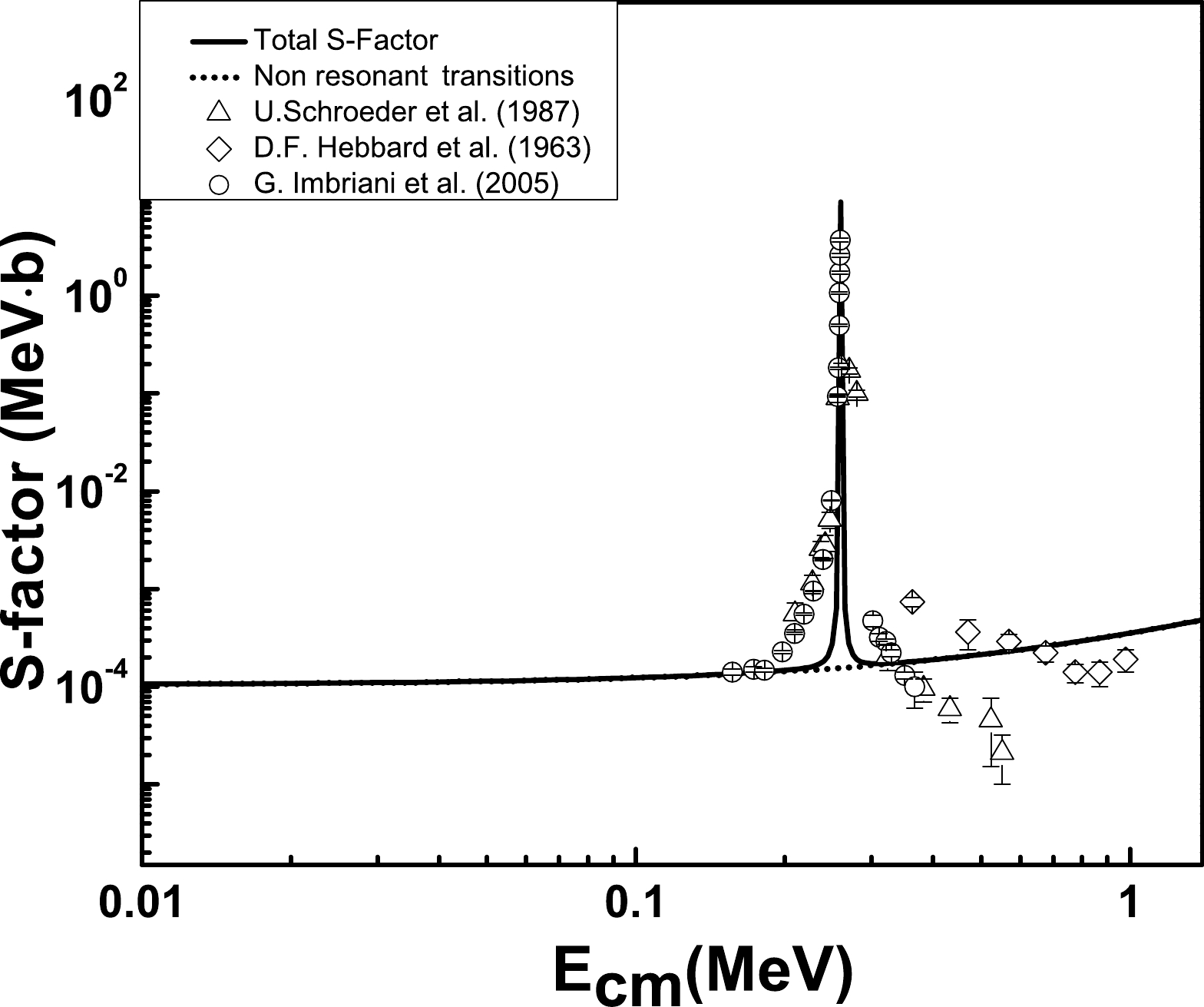
We employed the parameters reported in Table 2 for transitions to the third excited state at
$E_{x}$ =6.1763 MeV±1.7 keV. Our model-based results along with the measured data are presented in Fig. 2. The computed$ {{S}}_{6.176}(0) $ = 0.35495 keV·b. Comparison of${ {S}}_{6.176}(0)$ with the previous theoretical and experimental results is reported in Table 4. From Figs. 1 and 2, observe that we have obtained an accurate description of experimental astrophysical S-factors for radiative transitions to ground and third excited states of the 15O via PM, especially in the energy range Ecm ≤ 1.2 MeV. Note that both PM-based transitions from the continuum to the ground and third excited states are$ E1 $ resonant transitions.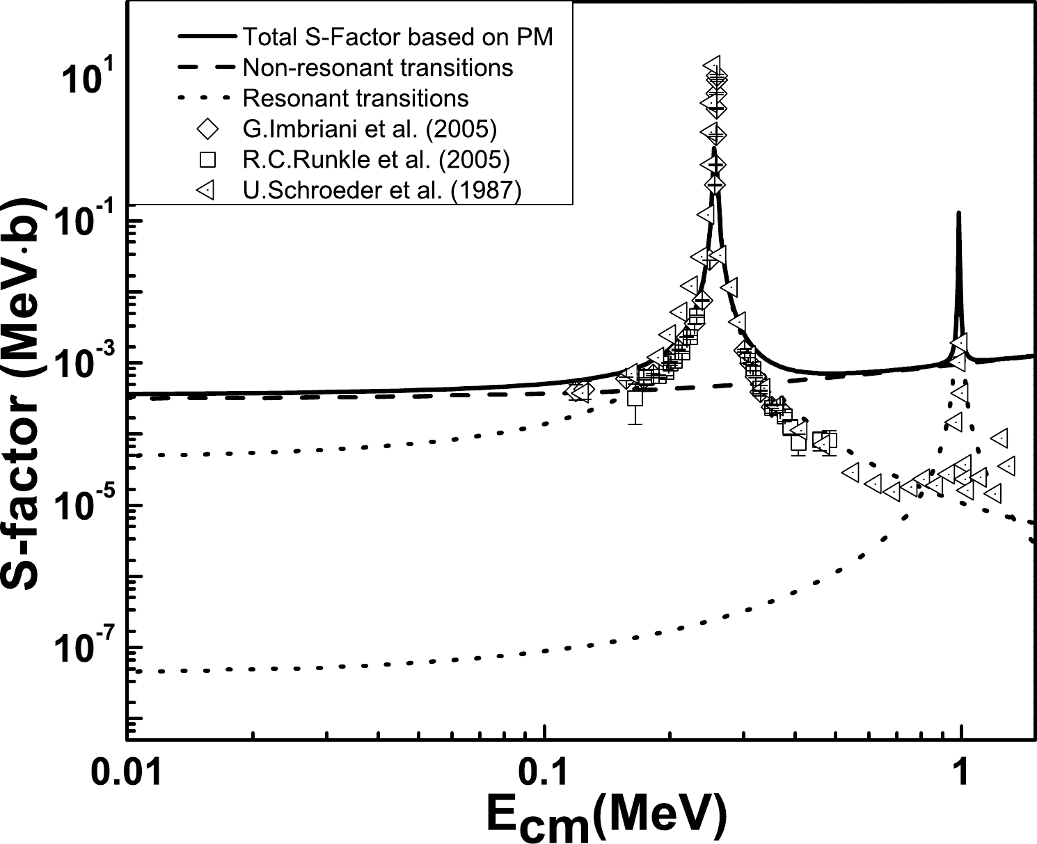
For the calculation of
$ M1 $ resonant transitions from the continuum to the first, second, fourth, and fifth excited states of$ ^{15}{\rm{O}} $ , we employed the R-matrix approach. The partial widths and channel radii of the resonant states are listed in Table 5. The transition from the J$ ^{\pi} $ =$ {1/2}^{+} $ ,$E_{x}$ =7.5565 MeV±0.4 keV to the first excited state of 15O along with the experimental data are displayed in Fig. 3. This transition may be fitted by including one resonance at$E_{\rm r}$ =0.259 MeV. The total S-factor of the radiative capture to the first excited state might be thought of as having a DC contribution. The resonant states and their parameters are reported in Table 5. Our computed${{S}}_{5.183}(0)= $ 0.10405 keV·b.Resonance State Bound state Γ /MeV $ \Gamma_{\gamma} $ /MeV

b/fm $ J_i^{\pi},$ 

$E_{\rm{r}} $ /MeV

$ J_f^{\pi},$ 

$\varepsilon_f $ /MeV

$ 1/2^{+} $ ,

0.259 $ 1/2^{+} $ ,

$ {2.114} $ 

0.987×10⁻³ 6.70×10⁻⁹ 6 $ 3/2^{+} $ ,

0.987 $ 5/2^{+} $ ,

$ {2.056} $ 

3.60×10⁻³ 0.41×10⁻⁶ 6 $ 1/2^{+} $ ,

0.259 $ 3/2^{+} $ ,

$ {0.504} $ 

0.987×10⁻³ 1.00×10⁻⁷ 6 $ 3/2^{+} $ ,

0.987 $ 5/2^{+} $ ,

$ {0.438} $ 

3.60×10⁻³ 0.01×10⁻⁶ 6 Table 5. The experimental data for total and radiative widths [33].
The transition to the second excited state is carried out by d-wave capture at the excitation energy
$E_{x}$ =8.2840 MeV±0.5 keV. The$ M1 $ resonant transition is computed from the continuum to the second excited state of 15O at$ E_{\rm{r}} $ =0.987 MeV. The parameters listed in Table 5 are employed for the R-matrix fittings. This transition has mixed contributions from the$ E1 $ non-resonant and$ M1 $ resonant. The R-matrix fit is attempted along with an external DC contribution yielding${{S}}_{5.24}(0)$ = 0.00981 keV·b, which is almost within the range of${{S}}_{5.24}(0)$ reported in Refs. [17, 23]. Our results are shown in Fig. 4 along with the measured data. The model-based computed results are well-fitted at the resonance point and its neighborhood.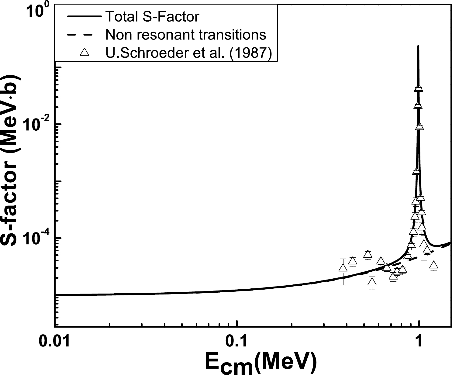
Figure 4. The 14N(p, γ)15O astrophysical S-factors of captures to the second excited state of
$E_{x}$ =5.2409 MeV. Comparison is shown with the measured data$ \bigtriangleup$ [11].In 14N(p, γ)15O, the transition to fourth excited state (
$E_{x}$ = 6.7931 MeV±1.7 keV) is crucial. Capture to$ J^{\pi} =$ $ 3/2^{+} $ has contributions from resonance capture through the first resonance$ M1 $ and direct$ E1 $ captures. The DC to the$E_{x}$ =6.7931 MeV±1.7 keV state is relatively peripheral because of its very small binding energy, and the${{S}}_{6.79}(0)$ is almost sensitive to the value of the channel radius$ R_N $ . The$E_{x}$ =6.7931 MeV±1.7 keV is described as an s-proton coupled to the core of 14N. The parameters reported in Table 5 are employed for the resonant capture. Note that the SF=1 is employed for this transition. However, Ref. [24] and Ref. [35] renormalized this value by multiplying the spectroscopic factor with their computed data, which in the case of Ref. [24] has a very small value. The results are depicted in Fig. 5 along with the experimental data. Our results show a better comparison with the experimental data at the resonance position and its neighborhood, where${{S}}_{6.79}(0)$ =0.83419 keV·b. The main contributions in the total S(0) come from the${{S}}_{\rm{g.s.}}(0)$ ,${{S}}_{6.17}(0)$ , and${{S}}_{6.79}(0)$ .
The transition to the fifth excited is carried out by d-wave capture at an excitation energy
$E_{x}$ =8.2840 MeV±0.5 keV. The resonance takes place at$ E_{\rm{r}} $ =0.987 MeV, the parameters of which are listed in Table 5. These parameters are employed for the R-matrix fittings. This transition has a significant role in$ E1 $ non-resonant capture and ($ E2+M1 $ ) resonant capture. The${{S}}_{6.68}(0)=$ 0.02971 keV·b. Our computed S-factor along with the experimental data are depicted in Fig. 6. In comparison to other transitions in 15O, the transition to the fifth excited state is rather weak. The transition to the sixth excited state is carried out by non-resonant captures. These transitions are very weak near zero energy; however, for energies exceeding than 0.5 MeV, their contribution should be accounted in the total S-factor. It is further mentioned in Fig. 7, where, at higher energies ($ E_{p}> $ 0.4 MeV), our computed results match well with the measured data. The${{S}}_{7.275}(0)$ =0.00523 keV·b.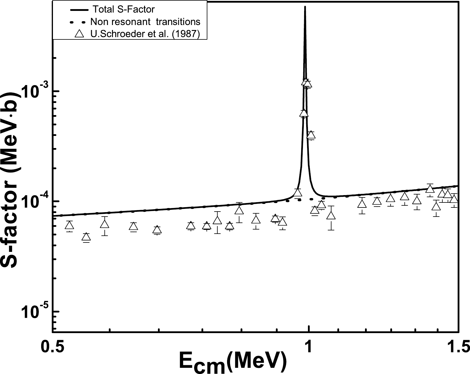
Figure 6. The 14N(p, γ)15O astrophysical S-factors of captures to the fifth excited state of
$ E_x $ =6.8594 MeV. Comparison is shown with the experimental data$ \bigtriangleup $ [11].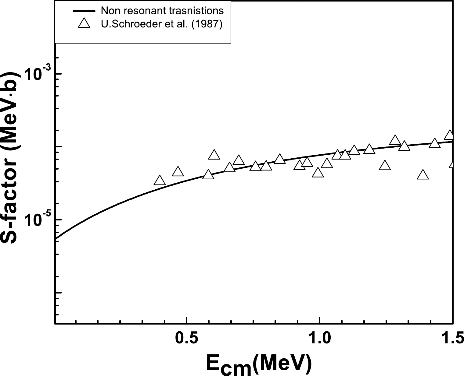
Figure 7. The 14N(p, γ)15O astrophysical S-factors of captures to the sixth excited state of
$ E_x $ =7.2759 MeV. Comparison is shown with the experimental data$ \bigtriangleup $ [11].The total S-factor is the sum of the partial S-factors for all possible resonants (
$ E1+E2+M1 $ ) and direct ($ E1 $ ) transitions. Our results for the total S-factor along with measured data are displayed in Fig. 8. The value of the total S-factor near zero energy is roughly 1.68641 keV·b. This value is also compared with existing theoretical and measured results reported in Table 4. We employed Eq. (16) for the polynomial fit between (0.001–0.10) MeV
$ S(E)= S(0)+ S^{'}(0)E+\frac{1}{2}S^{''}(0)E^2. $

(16) We obtained
$ S(0)=1.68\; {\rm{keV\cdot b}} $ ,$ S(0)^{'}=3.35\times 10^{-2}\; {\rm{b}}$ , and$ S(0)^{''}=2.17\times 10^{-4}\; {\rm{b/keV}} $ . Note that the contribution of the DC transition to the value of S(0) is almost 97%.The nuclear reaction rate for the
$ {p} + {^{14}\rm{N}} \rightarrow {^{15}\rm{O}+{\gamma}} $ process was calculated using Eq. (15). The results for the reaction rates are presented in Fig. 9 along with comparisons with previous calculations. These include the results obtained by Angulo et al. [14], Mukhamedzhanov et al. [15], Artemov et al. [23], Xu et al. [24], Frentz et al. [26], and Caughlan et al. [39]. Our computed rates are comparable with that those reported in Ref. [15] up to$ T_9 $ =0.1 with a percentage difference of approximately 19%. Our rates agree well with the higher rates reported in Ref. [24] at temperatures approaching$ T_9 $ =1. At$ T_9 $ =0.1, the difference between our computed rates and the higher rates reported in Ref. [24] is approximately 16.9%. At$ T_9 $ = 0.1, the rates obtained by Caughlan et al. [39] are improved by a factor of 1.18, with a percentage difference of 17.71%. At low temperatures,$ T_9 $ =0.1, the percentage difference between our model-based rates and those reported by Frentz et al. [26] is 12.98%.Table 6 compares our results with low, adopted, and high depicted in Ref. [24].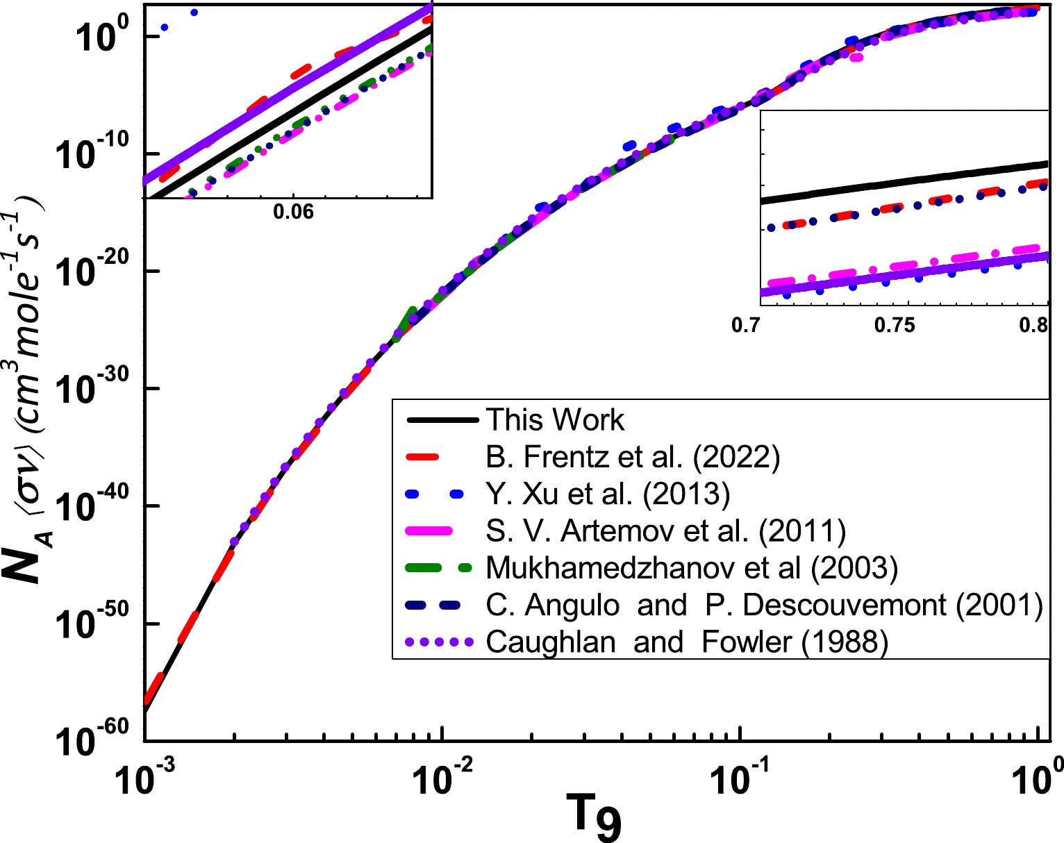
Figure 9. (color online) The calculated
$ {p} + {^{14}\rm{N}} \rightarrow {^{15}\rm{O}+{\gamma}} $ rate (solid line) in comparison to the rates computed by Angulo et al. [14] (short-dashes), Mukhamedzhanov et al. [15] (dash-dotted-dotted), Artemov et al. [23] (dash-dotted), Xu et al. [24] (dotted), Frentz et al. [26] (dashes), and Caughlan et al. [39] (short-dotted).Results from Ref. [24] This work ${T_{9} }$ 

$ \rm{Low} $ 

$ \rm{Adopted} $ 

$ \rm{High} $ 

0.008 $ 5.21\times 10^{-25} $ 

$ 5.84\times 10^{-25} $ 

$ 6.47\times 10^{-25} $ 

$ 6.80\times 10^{-25} $ 

0.009 $ 9.03\times 10^{-23} $ 

$ 1.01\times 10^{-23} $ 

$ 1.12\times 10^{-23} $ 

$ 1.17\times 10^{-23} $ 

0.010 $ 1.05\times 10^{-22} $ 

$ 1.18\times 10^{-22} $ 

$ 1.31\times 10^{-22} $ 

$ 1.36\times 10^{-22} $ 

0.011 $ 9.01\times 10^{-21} $ 

$ 1.01\times 10^{-21} $ 

$ 1.12\times 10^{-21} $ 

$ 1.16\times 10^{-22} $ 

0.012 $ 6.02\times 10^{-21} $ 

$ 6.74\times 10^{-21} $ 

$ 7.46\times 10^{-21} $ 

$ 7.79\times 10^{-21} $ 

0.013 $ 3.28\times 10^{-20} $ 

$ 3.68\times 10^{-20} $ 

$ 4.07\times 10^{-20} $ 

$ 4.25\times 10^{-20} $ 

0.014 $ 1.52\times 10^{-19} $ 

$ 1.70\times 10^{-19} $ 

$ 1.88\times 10^{-19} $ 

$ 1.96\times 10^{-19} $ 

0.015 $ 6.09\times 10^{-19} $ 

$ 6.82\times 10^{-19} $ 

$ 7.55\times 10^{-19} $ 

$ 7.89\times 10^{-19} $ 

0.016 $ 2.17\times 10^{-18} $ 

$ 2.43\times 10^{-18} $ 

$ 2.69\times 10^{-18} $ 

$ 2.81\times 10^{-18} $ 

0.018 $ 2.05\times 10^{-16} $ 

$ 2.30\times 10^{-16} $ 

$ 2.55\times 10^{-16} $ 

$ 2.66\times 10^{-17} $ 

0.020 $ 1.42 \times 10^{-15} $ 

$ 1.59\times 10^{-15} $ 

$ 1.76\times 10^{-15} $ 

$ 1.84\times 10^{-16} $ 

0.025 $ 6.82\times 10^{-15} $ 

$ 7.63\times 10^{-15} $ 

$ 8.45\times 10^{-15} $ 

$ 8.89\times 10^{-15} $ 

0.03 $ 1.30\times 10^{-13} $ 

$ 1.45\times 10^{-13} $ 

$ 1.61\times 10^{-13} $ 

$ 1.70\times 10^{-13} $ 

0.04 $ 9.45\times 10^{-11} $ 

$ 1.06\times 10^{-11} $ 

$ 1.17\times 10^{-11} $ 

$ 1.25\times 10^{-11} $ 

0.05 $ 1.98\times 10^{-10} $ 

$ 2.21\times 10^{-10} $ 

$ 2.45\times 10^{-10} $ 

$ 2.66\times 10^{-10} $ 

0.06 $ 2.01\times 10^{-09} $ 

$ 2.24\times 10^{-09} $ 

$ 2.47\times 10^{-09} $ 

$ 2.73\times 10^{-09} $ 

0.07 $ 1.27\times 10^{-08} $ 

$ 1.42\times 10^{-08} $ 

$ 1.57\times 10^{-08} $ 

$ 1.75\times 10^{-08} $ 

0.08 $ 5.83\times 10^{-08} $ 

$ 6.50\times 10^{-08} $ 

$ 7.17\times 10^{-08} $ 

$ 8.12\times 10^{-08} $ 

0.09 $ 2.12\times 10^{-07} $ 

$ 2.36\times 10^{-07} $ 

$ 2.60\times 10^{-07} $ 

$ 2.98\times 10^{-07} $ 

0.10 $ 6.48\times 10^{-07} $ 

$ 7.20\times 10^{-07} $ 

$ 7.92\times 10^{-07} $ 

$ 9.26\times 10^{-07} $ 

0.11 $ 1.78\times 10^{-06} $ 

$ 1.97\times 10^{-06} $ 

$ 2.16\times 10^{-06} $ 

$ 2.63\times 10^{-06} $ 

0.12 $ 4.75\times 10^{-06} $ 

$ 5.21\times 10^{-06} $ 

$ 5.66\times 10^{-06} $ 

$ 7.55\times 10^{-06} $ 

0.13 $ 1.31\times 10^{-05} $ 

$ 1.41\times 10^{-05} $ 

$ 1.52\times 10^{-05} $ 

$ 2.32\times 10^{-05} $ 

0.14 $ 3.79\times 10^{-05} $ 

$ 4.02\times 10^{-05} $ 

$ 4.25\times 10^{-05} $ 

$ 7.50\times 10^{-05} $ 

0.15 $ 1.09\times 10^{-04} $ 

$ 1.14\times 10^{-04} $ 

$ 1.20\times 10^{-04} $ 

$ 2.34\times 10^{-04} $ 

0.16 $ 3.00\times 10^{-04} $ 

$ 3.11\times 10^{-04} $ 

$ 3.23\times 10^{-04} $ 

$ 6.77\times 10^{-04} $ 

0.18 $ 1.77\times 10^{-02} $ 

$ 1.83\times 10^{-02} $ 

$ 1.88\times 10^{-03} $ 

$ 4.22\times 10^{-03} $ 

0.20 $ 7.65\times 10^{-02} $ 

$ 7.85\times 10^{-02} $ 

$ 8.05\times 10^{-03} $ 

$ 1.86\times 10^{-02} $ 

0.25 $ 1.06\times 10^{-01} $ 

$ 1.09\times 10^{-01} $ 

$ 1.11\times 10^{-01} $ 

$ 2.64\times 10^{-01} $ 

0.30 $ 5.91\times 10^{-01} $ 

$ 6.05\times 10^{-01} $ 

$ 6.19\times 10^{-01} $ 

$ 1.48\times 10^{+00} $ 

0.35 $ 1.95\times 10^{+00} $ 

$ 2.00\times 10^{+00} $ 

$ 2.04\times 10^{+00} $ 

$ 4.93\times 10^{+00} $ 

0.40 $ 4.66\times 10^{+00} $ 

$ 4.77\times 10^{+00} $ 

$ 4.88\times 10^{+00} $ 

$ 1.18\times 10^{+01} $ 

0.45 $ 8.99\times 10^{+00} $ 

$ 9.20\times 10^{+00} $ 

$ 9.41\times 10^{+00} $ 

$ 2.28\times 10^{+01} $ 

0.50 $ 1.50\times 10^{+01} $ 

$ 1.53\times 10^{+01} $ 

$ 1.57\times 10^{+01} $ 

$ 3.81\times 10^{+01} $ 

0.60 $ 3.11\times 10^{+01} $ 

$ 3.18\times 10^{+01} $ 

$ 3.25\times 10^{+01} $ 

$ 7.92\times 10^{+01} $ 

0.70 $ 5.06\times 10^{+01} $ 

$ 5.18\times 10^{+01} $ 

$ 5.31\times 10^{+01} $ 

$ 1.29\times 10^{+02} $ 

0.80 $ 7.13\times 10^{+01} $ 

$ 7.31\times 10^{+01} $ 

$ 7.48\times 10^{+01} $ 

$ 1.82\times 10^{+02} $ 

0.90 $ 9.15\times 10^{+01} $ 

$ 9.39\times 10^{+01} $ 

$ 9.62\times 10^{+01} $ 

$ 2.34\times 10^{+02} $ 

1.00 $ 1.10\times 10^{+02} $ 

$ 1.14\times 10^{+02} $ 

$ 1.17\times 10^{+02} $ 

$ 2.85\times 10^{+02} $ 

Table 6. The radiative capture rates of 14N(p, γ)15O(cm3 s-1 mol-1).
-
Massive main sequence stars (particularly those nearing the end of their lives) and red giants generate energy via the CNO cycle. The 14N(p, γ)15O reaction influences the rate of energy and neutrino production in the CNO cycle. During the transition period from the main sequence to the red giants, few factors, including the stellar structure and luminosity, are affected by 14N(p, γ)15O. The CNO neutrino production increases owing to the decay of 15O because the solar 15O decay rate correlates directly with the 14N(p, γ)15O production rate.
We analyzed the astrophysical S-factor and nuclear reaction rates for resonant and non-resonant transitions using the PM and R-matrix approach. The possible
$ E1 $ transitions were computed employing the PM for the DC, whereas$ M1 $ transitions were calculated using the R-matrix approach. The Woods-Saxon potential was employed as a nuclear input to calculate the bound and scattering state wave functions. The position of resonance was accurately determined by our chosen parameters for the Woods-Saxon potential. The computed S-factors were consistent with the previous reported results at and nearby the resonance.Owing to the poor description of the M1 resonant transition by the PM method, the transitions from
$ J^{\pi} $ =$ 1/2^{+} $ at$E_{x}$ =7.5565 MeV±0.4 keV and from$ J^{\pi} = 3/2^{+} $ at$E_{x}$ =8.2840 MeV±0.5 keV to the first, second, fourth, and fifth excited states were computed using the R-matrix approach. The computed S-factor for these transitions agreed more with the measured data. The computed S(0) values were compared with previous measured and calculated results in Table 4. Based on the total cross-section, we computed the rates for all possible transitions. The present model-based rates confirm that the 14N(p, γ)15O is the slowest process among the capture processes of the CNO cycle. The$ {p} + {^{14}\rm{N}} \rightarrow {^{15}\rm{O}+{\gamma}} $ reaction rates mainly affect the luminosity of the horizontal branch and age of the stars. Our calculations demonstrate the possibility of describing the process of radiative capture of a proton by the 14N nucleus, assuming the value of the spectroscopic factor equal to unity.
Radiative capture of proton through the 14N(p,γ)15O reaction at low energy
- Received Date: 2023-08-31
- Available Online: 2024-04-15
Abstract: The CNO cycle is the main source of energy in stars more massive than our Sun. This process defines the energy production, the duration of which can be used to determine the lifetime of massive stars. The cycle is an important tool for determining the age of globular clusters. Radiative proton capture via


 DownLoad: