


 Abstract
 HTML
HTML Reference
 Related
 PDF
PDF


-
Deep inelastic scattering (DIS) process is used to study the internal structure of protons [1], which is a puzzle in quantum chromodynamics (QCD). The main difficulty emanates from the fact that massless gluons and nearly massless quarks give rise to the mass of the proton
$ M\sim 1 \;\rm GeV $ . One can say that from the perspective of special relativity, the missing mass could be due to the kinetic energy of quarks and gluons inside the proton; however, the mentioned kinetic energy is insufficient to describe the total vanishing mass. To learn more about this topic, breaking the conformal symmetry in QCD is another reason that should be considered. It leads to anomalous dimension contributions in the DIS. Recall that QCD coupling is large at low energies; hence, perturbation calculations cannot be used to study many properties of hadrons. Therefore, an alternative way to study DIS is to use a holographic approach.In AdS/CFT description, a strongly coupled field theory at the boundary of the AdS space can be described using a weakly coupled gravitational theory in bulk AdS [2, 3]. In other words, a ten-dimensional geometry at the corresponding boundary is an exact dual of a supersymmetric
$S U(N)$ gauge theory with large N in the bulk. In particular, the string theory in the${\rm AdS}_5\times S_5$ space is a dual of a four-dimensional gauge theory. AdS/CFT duality has originally been considered for conformal theories; however, it has been generalized to non-conformal theories such as QCD. Therefore, in any case of interest, a QCD problem can be studied by assuming an appropriate AdS background. In the current holographic study, a DIS process with a proton target is considered using a modified${\rm AdS}_5$ background. In a phenomenological holographic approach, AdS/QCD attempts to adapt a five-dimensional effective field theory to QCD as much as possible. Therefore mass gap, confinement, and supersymmetry breaking are obtained by considering modifications in gravitational duals. To break the conformal symmetry, one can modify the radial coordinate, which is the 5th dimension of spacetime, as discussed in reference [4]. In the AdS/QCD approach, the anomalous dimension associated with DIS is replaced by introducing a modification parameter in the gravity dual. Because of this, a holographic modified model can deal with phenomenological aspects of DIS. An anomalous dimension is introduced into the holographic context to fit the masses for mesons, baryons, and glueballs [5–7]. The correct modification parameter value in different models can be determined using phenomenology to set the values of known physical quantities. For example, one may adopt a modified AdS that introduces the gluon condensation on the QCD side of duality.Originally, gluon condensation was a measure of the non-perturbative physics in zero-temperature QCD [8]. It was later identified as an order parameter for confinement to study certain non-perturbative phenomena [9–12]. The gluon condensate
$ G_2 $ is the vacuum expectation value of the operator$ \frac{\alpha_s}{\pi} G^a_{\mu\nu}G^{a,\mu\nu} $ , where$ G^a_{\mu\nu} $ is the gluon field strength tensor. A non-zero trace of the energy-momentum tensor appears in a full quantum theory of QCD. The anomaly implies a non-zero gluon condensate, which can be calculated as [13–15],$ \begin{align} \Delta G_2(T)= G_2(T)-G_2(0)=-(\varepsilon(T)-3\;P(T)), \end{align} $

(1) where
$ G_2(T) $ denotes the thermal gluon condensate;$ G_2(0) $ , which is equal to the condensate value at the deconfinement transition temperature, is the zero temperature condensate vale;$ \varepsilon(T) $ is the energy density; and$ P(T) $ is the pressure of the QGP system.A well-known modified holographic model introducing gluon condensation in the boundary theory is given by the following background metric in the Minkowski spacetime [16],
$ \begin{aligned}[b] {\rm d}s^2=& g_{mn}\; {\rm d}x^{m}\; {\rm d}x^{n}\\=&\frac{L^2}{z^2}\Bigg(\sqrt{1-c^2 z^8}\Bigg(-{\rm d}t^2+\sum_{i}{\rm d}x_i^2\Bigg)+{\rm d}z^2\Bigg), \end{aligned} $

(2) $ \varphi(z)=\sqrt{\frac{3}{2}} \ln \dfrac{1+cz^4}{1-cz^4}+\varphi_0. $

(3) In the above dilaton-wall solution,
$ i = 1,2,3 $ are orthogonal spatial boundary coordinates, z denotes the$ 5 $ th dimension radial coordinate, and$ z=0 $ sets the boundary.$ \varphi_0 $ is a constant,$ c=\dfrac{1}{z^4_c} $ , and$ z_{c} $ denotes the IR cutoff. It shows that z is defined from zero to the IR limit as usual. To clarify, parameter c does not bound the upper limit of z to values less than the cutoff; in fact, it should be interpreted as$ c<\dfrac{1}{z^4} $ . In other words, for a very large value of z, the parameter c tends to an infinitesimal value based on the range$ 1-c^2z^8>0 $ . Furthermore, we perform calculations in the unit where L = 1. To investigate the appearance of the forth correction of radial coordinate (with the coefficient denoted as c) in the metric, it is worth mentioning that the dilaton field is dual to a scalar operator and the metric is dual to the energy-momentum tensor of the dual field theory [17] (discussion further in [18, 19]). Expanding the dilaton profile near$ z = 0 $ will give$ \begin{align} \varphi(z)=\varphi_0+\sqrt{6} c z^4+.... \end{align} $

(4) According to the holographic dictionary, φ and c are the source and parameter associated with the confinement, respectively. We expect the constant piece to correspond to the source for the operator
$ TrG_2 $ and coefficient of$ z_4 $ to give the gluon condensate [20]. It is evident that c in the background metric breaks the conformal symmetry; hence, the gluon condensation appears in the boundary theory. The relevant phenomenological information shows that its value lies in the range$ 0< c\leq 0.9 \; \rm GeV^4 $ [21–23], and recent lattice calculations based on a QCD sum rule method show that the gluon condensate behaves as a rapid change around$ T_c $ [24, 25]. We are interested in obtaining the exact value of c in a proton-targeted DIS process.The holographic description of the gluon condensation allows several physical quantities to be studied in this context. First, to familiarize with its phenomenological aspects, it should be noted that the dilaton wall solution represented by (2), (3) is related to the zero temperature case; hence, this is suitable for studying DIS and its physics. As expected, one can readily confirm that in the limit
$ c\longmapsto 0 $ , (2) reduces to$\rm AdS_5$ which does not present the mass gap, whereas the modification of the radial coordinate can yield more phenomenological results. In fact, it has become an approach to discuss more phenomenological aspects using modified AdS [26–28].In a work related to our study [29], such a scattering was investigated using a deformed AdS. Since models with anomalous dimension in AdS/QCD lead to mass-scale fermionic field generation, several works have employed them to solve DIS [29–61]. In view of all the abovementioned motivations, we will use a holographic model of gluon condensation, given by (2) and (3), to study DIS with the proton target.
This remainder of this paper is structured as follows. After a brief overview of the DIS properties using holography in Sec. II, we study the electromagnetic interactions and baryonic states in deep inelastic scattering in Secs. III and IV, respectively. Based on these results, Sec. V presents the interaction action, and subsequently, we discuss the structure functions according to the relationship between the action and scattering amplitude. In Sec. VI, we briefly review and discuss our results.
-
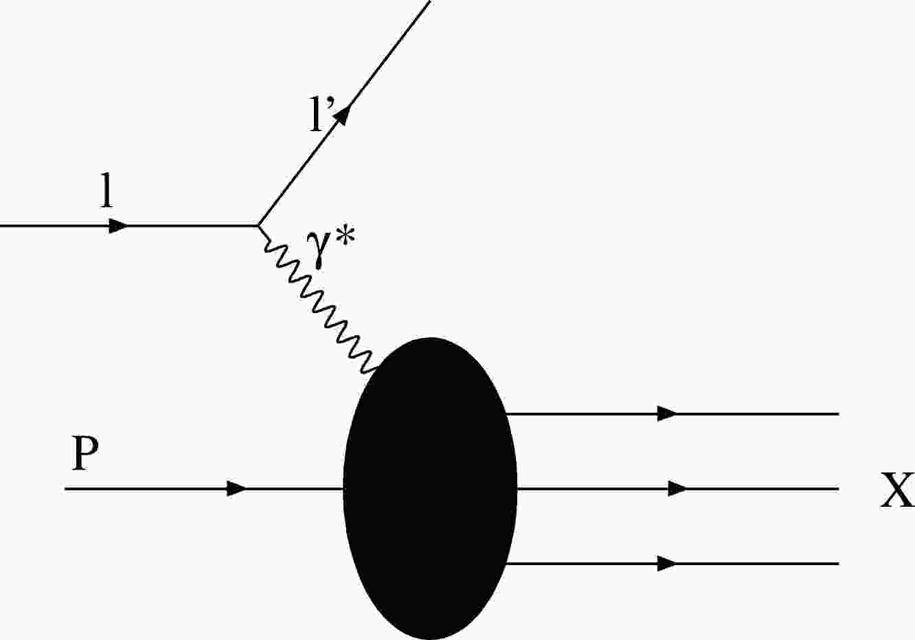
First, a brief overview of deep inelastic scattering is provided to clarify our motivation and goals. The main application of DIS in particle physics is to study the internal hadronic structure and strong interactions. Consider a DIS process in which a lepton is scattered off a proton target, as shown in Fig. 1. During this scattering, a virtual photon is exchanged. Proton fragmentation creates a lepton and some final hadronic states. It should be noted that the production of final hadronic states depends on the four momentums of the initial lepton transfers. Therefore, the four momentums leads to the expulsion of inner quarks and gluons of the proton. Finally, the quark anti-quark pairs are hadronized. According to Ref. [62], DIS is parametrized using the Bjorken dynamical variable which is defined as

Figure 1. Deep inelastic scattering process of the lepton on the proton by exchange of the virtual photon.
$ \begin{align} x=-\frac{q^2}{2P \cdot q}, \end{align} $

(5) where q is the momentum transferred by the lepton to the proton target via a virtual photon and P is the initial momentum of the proton. We adopt the method explained in [62] and rederived in [5, 29]. Hence, the hadronic transition amplitude is given as
$ W^{\mu\nu}=F_1 \left(\eta^{\mu\nu}-\frac{q^{\mu}q^{\nu}}{q^2}\right)+\frac{2x}{q^2} F_2 \left(P^{\mu}+\frac{q^{\mu}}{2x}\right)\left(P^{\nu}+\frac{q^{\nu}}{2x}\right), $

(6) where
$ F_{1,2}=F_{1,2}(x,q^2) $ are structure functions.Next, we relate the abovementioned matrix to holography. From the AdS/QCD dictionary, elements of (6) on the QCD side are associated with the interaction action on the AdS side as [30],
$ \begin{align} \eta_{\mu}<P+q,s_{X}\vert J^{\mu}(0)\vert P,s_i>={\cal{K}}_{{\rm eff}}S_{{\rm int}}, \end{align} $

(7) where
$ \eta_{\mu} $ is the polarization of the virtual photon,$ \vert P,s_i> $ represents a normalizable proton state with spin$ s_i $ ,$ J^{\mu} $ is the electromagnetic quark current, and$ s_X $ denotes the final state. It is worth mentioning that$ {\cal{K}}_{{\rm eff}} $ is an effective factor that adjusts the bulk supergravity quantities to the boundary phenomenologically. This is based on a different perspective presented in Ref. [5] that the bulk/boundary quantities of (7) are proportional and not necessarily equal.The interaction action is written as
$ \begin{align} S_{{\rm int}}=g_{V}\int {\rm d}z {\rm d}^4y {\rm e}^{-\varphi}\sqrt{-g}\phi^{\mu} \bar{\Psi}_{X}\Gamma_{\mu}\Psi_{i}, \end{align} $

(8) where
$ g_V $ is a coupling constant related to the electric charge of the baryon, φ is the dilaton field,$ \sqrt{-g} $ is given by the metric,$ \phi^{\mu} $ is the electromagnetic gauge field,$ \Psi_{i} $ and$ \Psi_{X} $ are the initial and final state spinors for the baryon, respectively, and$ \Gamma_{\mu} $ are Dirac gamma matrices in the curved space. By computing all the above quantities according to (2) and (3), the interaction action of DIS can be studied. -
A photon is exchanged during scattering, hence, we study the electromagnetic interactions in the bulk. It can be described as the presence of photon in the modified AdS. The action of a five-dimensional massless gauge field
$ \phi^{n} $ is given by$ \begin{align} S= -\frac{1}{4}\int {\rm d}^5x {\rm e}^{-\varphi}\sqrt{-g} F^{mn}F_{mn}, \end{align} $

(9) where
$ F^{m n}=\partial^{m} \phi^{n}-\partial^{n} \phi^{m} $ with m,n representing the 5-dimensional space including the Minkowski spacetime coordinates,$ \mu,\nu $ , and z; and$ {\varphi} $ is the dilaton field given by (3). Note that$ {\varphi} $ and ϕ should be differentiated. In fact (9) is an action showing the gauge field ϕ on a background coupled to a dilaton field$ {\varphi} $ . From (9), the equation of motion of such an electromagnetic field is derived as$ \begin{align} \partial_{m}[{\rm e}^{-\varphi}\sqrt{-g}F^{mn}]=0. \end{align} $

(10) Considering
$ m,n\equiv \mu,\nu, z $ , the relation (10) leads to$ \begin{aligned}[b] \partial_{\mu}\Bigg[\frac{1}{z}(1+cz^4)^{1-\sqrt{\frac{3}{2}}}(1-cz^4)^{1+\sqrt{\frac{3}{2}}}F^{\mu z}\Bigg]=0, \end{aligned} $

$ \begin{aligned}[b] \partial_{z}\Bigg[\frac{1}{z}(1+cz^4)^{1-\sqrt{\frac{3}{2}}}(1-cz^4)^{1+\sqrt{\frac{3}{2}}}F^{z \mu}\Bigg]=0. \end{aligned} $

(11) To solve the equations of motion of the gauge field in (11), we first fix the gauge. Suppose there is an electromagnetic field in the bulk defined with the metric (2). This obeys the 5–dimensional Maxwell equation supplemented by a gauge condition, which we take to be
$ \begin{align} {\rm e}^{-\varphi}\sqrt{-g}\partial_{\mu}\phi^{\mu}+\partial_{z}({\rm e}^{-\varphi}\sqrt{-g}\phi_{z})=0. \end{align} $

(12) From (12), one can write
$ \begin{aligned}[b]\\[-8pt] \partial_{\mu}\phi^{\mu}+\frac{z}{(1+cz^4)^{1-\sqrt{\frac{3}{2}}}(1-cz^4)^{1+\sqrt{\frac{3}{2}}}}\partial_{z}\Bigg{(}\frac{(1+cz^4)^{1-\sqrt{\frac{3}{2}}}(1-cz^4)^{1+\sqrt{\frac{3}{2}}}}{z}\phi_{z}\Bigg{)}=0, \end{aligned} $ 
(13) hence,
$ \begin{align} \square \phi_{\mu}+\partial_{\mu}\partial_{z}\phi_{z}-\frac{1+4\sqrt{6}cz^4+7c^2z^8}{z(1-c^2z^8)}\partial_{\mu}\phi_{z}=0. \end{align} $

(14) Using the gauge (14) together with (11) leads to the following equations,
$ \begin{align} \square \phi_{z}-\partial_{\mu}\partial_{z}\phi^{\mu}=0, \end{align} $

(15) $ \begin{align} \square \phi_{\mu}+\partial^2_{z}\phi_{\mu}-\frac{1+4\sqrt{6}cz^4+7c^2z^8}{z(1-c^2z^8)} \partial_{z}\phi_{\mu}=0. \end{align} $

(16) At this point, one can consider a photon with a particular polarization as
$ \eta_{\mu}q^{\mu}=0 $ for simplicity; hence, only the$ \phi^{\mu} $ component contributes to the scattering [5, 30, 33]. In the latter case, we need to solve only (16). This equation cannot be solved analytically; hence, we use numerical methods. Let us consider$ \phi_{\mu}(z,q,y)=\eta_{\mu} {\rm e}^{{\rm i}q.y} \phi_{1}(z,q) $ , and the condition$ \phi_{\mu}(z,q,y)\vert_{_{z=0}}=\eta_{\mu} {\rm e}^{{\rm i}q.y} $ in (16). We use reference [5] for the initial condition, because we should obtain similar results at the boundary$ z=0 $ . At the IR limit we take the Neumann boundary condition. Therefore,$ \phi_{1}(z,q) $ should be convergent and the assumption is taken as follows:$ \dfrac{\partial \phi_1}{\partial z}\mid_{z=z_c}=0 $ . Then, we can obtain$ \phi_{1}(z,q) $ versus z that describes the behaviour of the electromagnetic field in the bulk. Figure 2 shows$ \phi_1(z,q) $ for different values of$ q^2 $ and c. Plot (a) shows that for large values of$ q^2 $ , increasing the parameter c does not affect$ \phi_1(z,q) $ significantly. In addition,$ \phi_1 $ has its maximum value near the boundary$ (z=0) $ . In plot (b), for small values of$ q^2 $ , increasing the parameter c increases the magnitude of$ \phi_1 $ , which is more visible with large values of z. Plot (c) is a comparison of$ \phi_1 $ at different values of$ q^2 $ and a fixed c. It is evident that$ \phi_1 $ is stronger when$ q^2 $ is smaller. In other words, the magnitude of the electromagnetic field is larger for smaller values of$ q^2 $ .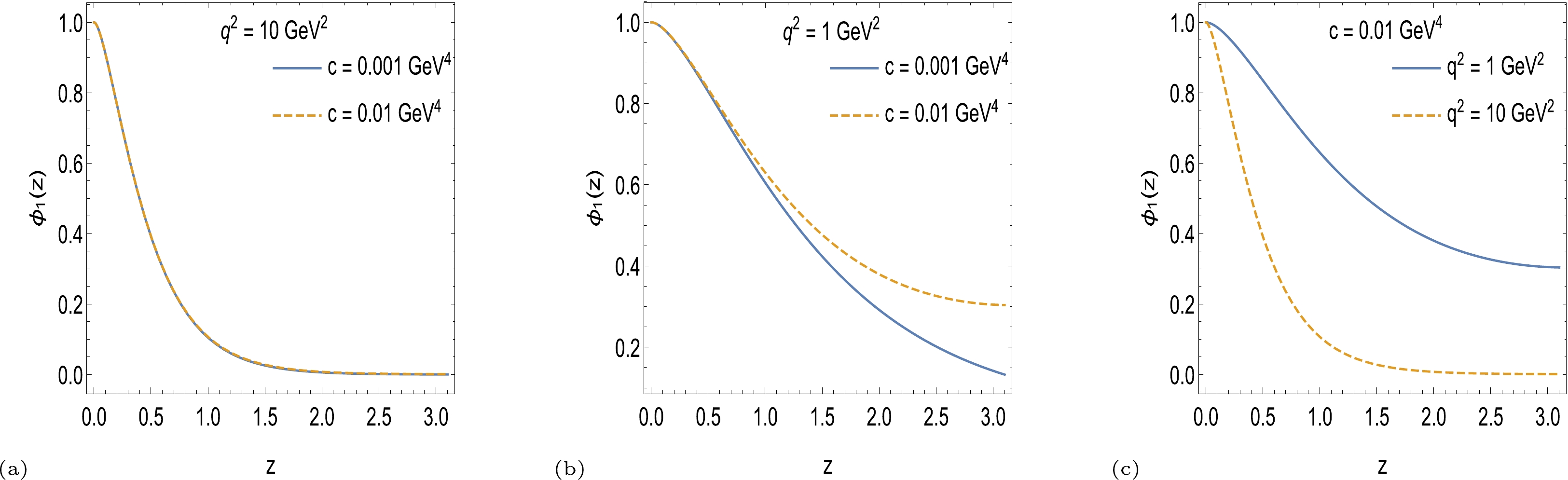
Figure 2. (color online) Electromagnetic field in the bulk with (a) large value of
$q^2=10\; {\rm GeV}^2$ and two different values of$c=0.01\; {\rm GeV}^4$ and$c=0.001\; {\rm GeV}^4$ , (b) small value of$q^2=1 \;{\rm GeV}^2$ and two different values of$c=0.01\; {\rm GeV}^4$ and$c=0.001\; {\rm GeV}^4$ , (c) two different values of parameter$q^2=1\; {\rm GeV}^2$ and$q^2=10 \;{\rm GeV}^2$ at fixed value of$c=0.01\; {\rm GeV}^4$ . -
In this section, we study the baryonic initial and final states for further requirements of the interaction action (8). The action for the fermionic fields is written as
$ \begin{align} S=\int {\rm d}x^5 {\rm e}^{-\varphi} \sqrt{g} \Psi(\not D-m_5)\Psi. \end{align} $

(17) where
$ m_5 $ is the baryon bulk mass and the operator$ {\not D} $ is defined as$ \begin{align} \not D= g^{mn} e^{a}_{n} \gamma_{a}\left(\partial_{m}+\frac{1}{2}\omega^{bc}_{m}\Sigma_{bc} \right), \end{align} $

(18) in which
$ g^{mn} $ is given by metric (2),$ \gamma_{\alpha}=(\gamma_{\mu},\gamma_{5}) $ ,$ \lbrace\gamma_{a},\gamma_{b}\rbrace=2\eta_{ab} $ and$ \Sigma_{\mu 5}= \dfrac{1}{4}[\gamma_{\mu},\gamma_{5}] $ [63–67].$ \gamma_{\mu} $ are Dirac's gamma matrices. a, b, c are flat spaces, and m, n, p, q are AdS space indices. As before,$ \mu, \nu $ represent the Minkowski space. The equations of motion of fermionic states are$ \begin{align} (\not D-m_5)\Psi=0. \end{align} $

(19) With the metric (2), vielbeins are computed as
$ \begin{aligned}[b] e^a_n=&\frac{(1-c^2 z^8)^{\frac{1}{4}}}{z}\delta^{a}_n,\\ a=&t,x_1, x_2, x_3,\\ e^b_n=&\frac{1}{z}\delta^{b}_n, \\ b=&z. \end{aligned} $

(20) The above terms give us the first term of (18). Now, we calculate the second term. Spin connection is given by
$ \begin{align} \omega^{ab}_{m}=e^a_n\partial_m e^{nb}+e^a_n e^{pb}\Gamma^{n}_{pm}, \end{align} $

(21) where the Christoffel symbols are
$ \begin{align} \Gamma^{p}_{mn}=\frac{1}{2}g^{pq}(\partial_n g_{mq}+\partial_m g_{nq}- \partial_q g_{mn}). \end{align} $

(22) From the metric (2), one may write
$ g_{\mu\nu}=\dfrac{\sqrt{1-c^2z^8}}{z^2}\eta_{\mu\nu} $ and$ g_{zz}=\dfrac{1}{z^2} $ . Hence, the only non-vanishing terms are$ \Gamma^{p}_{mn}\Rightarrow \Gamma^{z}_{\mu\nu}, \Gamma^{z}_{zz},\Gamma^{\mu}_{\nu z} $ . After computation, they are written as$ \begin{aligned}[b] \Gamma^{z}_{\mu\nu}=&- \frac{(1+c^2z^8)}{z(1-c^2z^8)}\eta_{\mu\nu}\\ \Gamma^{z}_{zz}=&\frac{1}{z} \\ \Gamma^{\mu}_{\nu z}=& \frac{(1+c^2z^8)}{z(1-c^2z^8)}\delta^{\mu}_{\nu}. \end{aligned} $

(23) In addition, from (2) combined with (20) and (22), the relation (21) turns to
$ \begin{align} \omega^{z\nu}_{\mu}=-\omega^{\nu z}_{\mu}=-\frac{(1+c^2z^8)}{z(1-c^2 z^8)^{\frac{3}{4}}}\delta^{\nu}_{\mu}, \end{align} $

(24) hence, other components of
$ \omega^{ab}_{m} $ are zero. Using these solutions, (18) is given by$ \begin{align} {\not D}=z \gamma^5 \partial_z+ \frac{z}{(1-c^2z^8)^{\frac{1}{4}}} \gamma^{\mu}\partial_{\mu}-2\frac{(1+c^2z^8)}{z(1-c^2 z^8)^{\frac{3}{4}}}\gamma^5, \end{align} $

(25) and (19) is written as
$ \begin{aligned}[b] \left[z \gamma^5 \partial_z+ \frac{z}{(1-c^2z^8)^{\frac{1}{4}}} \gamma^{\mu}\partial_{\mu}-2\frac{(1+c^2z^8)}{z(1-c^2 z^8)^{\frac{3}{4}}}\gamma^5-m_5\right]\Psi=0. \end{aligned} $

(26) Since the spinor is either left-handed or right-handed, and since Kaluza-Klein modes are dual to the chirality spinors, these components are decomposed and expanded as
$ \begin{align} \Psi_{L/R}(x^{\mu},z)=\Sigma_{n} f^n_{L/R}(x^{\mu})\chi^n_{L/R}(z), \end{align} $

(27) and by applying (27) in the equation of motion (26), we obtain the coupled equations as
$ \left(\partial_{z}-2\frac{(1+c^2z^8)}{z^2(1-c^2z^8)^{\frac{3}{4}}}+\frac{m_5}{z}\right)\chi_{_{L}}(z)=\frac{M_n}{(1-c^2z^8)^{\frac{1}{4}}}\chi_{_{R}}(z), $

(28) $ \left(\partial_{z}-2\frac{(1+c^2z^8)}{z^2(1-c^2z^8)^{\frac{3}{4}}}-\frac{m_5}{z}\right)\chi_{_{R}}(z)=\frac{-M_n}{(1-c^2z^8)^{\frac{1}{4}}}\chi_{_{L}}(z). $

(29) Decoupling (28) and (29) leads to the following equation, which describes both left-handed and right-handed sectors as
$ \begin{aligned}[b]& -(1-c^2z^8)^{\frac{1}{4}}\Big{(}\partial_{z}-2\frac{(1+c^2z^8)}{z^2(1-c^2z^8)^{\frac{3}{4}}}\pm\frac{m_5}{z}\Big{)}\\&\times(1-c^2z^8)^{\frac{1}{4}}\Big{(}\partial_{z}-2\frac{(1+c^2z^8)}{z^2(1-c^2z^8)^{\frac{3}{4}}}\mp\frac{m_5 }{z}\Big{)}\chi_{_{R/L}}(z)\\ =&M_n^2 \chi_{_{R/L}}(z). \end{aligned} $

(30) Below, we create a Schrödinger-like equation by applying a transformation similar to
$ \begin{align} \chi_{_{R/L}}(z)= \frac{{\rm e}^{-\frac{2(1-c^2z^8)^{\frac{1}{4}}}{z}}}{(1-c^2z^8)^{\frac{1}{8}}}\psi_{_{R/L}}(z), \end{align} $

(31) hence, Eq. (30) is written as
$ \begin{align} \sqrt{1-c^2z^8}\Big{(}-\psi''_{R/L}(z)+\frac{m_5(m_5\mp 1)-c^2z^8(2m^2_5+7)+c^4z^{16}m_5(m_5\pm 1)}{z^2(1-c^2z^8)^2}\psi_{R/L}(z)\Big{)}=M_n^2 \psi_{R/L}(z) \end{align} $

(32) In (32),
$ m_5 $ is a parameter on the AdS side of the gauge/ gravity duality and is related to the baryon mass on the gauge side; hence, the normalizable solutions of the equations above are dual to the states in the boundary theory. In pure AdS space, the bulk mass is related to the canonical conformal dimension$\Delta_{\rm can}$ of a boundary operator as$ \begin{align} |m^{{\rm AdS}}_5|=\Delta_{{\rm can}}-2. \end{align} $

(33) Recall that
$\rm QCD$ is not a conformal field theory since it has a mass gap. Hence, the gravity side should be modified, resulting in an unpure AdS. If AdS is modified, the canonical dimension$\Delta_{\rm can}$ of an operator has an anomalous contribution γ, implying an effective scaling dimension.$ \begin{align} |m_5|=\Delta_{{\rm can}}+\gamma-2. \end{align} $

(34) The contribution of the anomaly is related to how one modifies the theory. For example, in Ref. [5], the modification of the scale introduces the mass gap in the theory. Therefore, the anomalous contribution represents the energy scale in the theory and leads to the mass spectra. Hence, the main task is to find the value of the bulk mass in (34). In AdS/CFT dictionary, when the bulk mass is related to the dimension, it means that the energy scale of the boundary theory is holographically related to the localization in the z-coordinate; therefore, we have z-dependent mass in the bulk. Let us focus on
$ m_5 $ . One can fit$ m_5 $ numerically as Eq. (32) has normalizable solutions. By fixing M as the proton mass, we should find suitable values for c and$ m_5 $ , which give us well-defined solutions.Figures 3 and 4 show the initial (n=1) and final (for two excited states as n=2, 3) chiral components of the wave function. To solve Eq. (32) numerically, we fix proton mass M as the eigenvalue of the equation; therefore,
$ m_5 $ and c are found as$ c=0.0120 \; \rm GeV^4 $ and$ m_5=0.081 \; \rm GeV $ . Interestingly, the value of parameter c on the AdS side is close to the phenomenological GC value of QCD as found$ G_2 = 0.010 \pm 0.0023 \; \rm GeV^4 $ in Ref. [26]. Another consequence of the presence of c is that the anomaly γ in (34) affects the bulk mass intensely. After obtaining both left-handed and right-handed modes from (32), we have
Figure 3. (color online) Left-handed (dashed) and right-handed (solid) sectors of wave function from (32) for the initial state (target proton), by considering
$ c=0.0120 \; \rm GeV^4 $ and$ m_5= $ 0.081 GeV.
Figure 4. (color online) Left-handed (dashed) and right-handed (solid) sectors of wave function from (32) for the final state (a) n=2 and (b) n=3, by considering
$ c=0.0120 \;\rm GeV^4 $ and$ m_5=0.081\;\rm GeV $ .$ \begin{align} \Psi_i= \frac{{\rm e}^{-\frac{2(1-c^2z^8)^{\frac{1}{4}}}{z}}}{(1-c^2z^8)^{\frac{1}{8}}} {\rm e}^{{\rm i}P.y}[(\frac{1+\gamma_5}{2})\psi^i_L+(\frac{1-\gamma_5}{2})\psi^i_R] u_{s_i}(p), \end{align} $

(35) as the initial wave function for the target proton and
$ \begin{align} \Psi_X= \frac{{\rm e}^{-\frac{2(1-c^2z^8)^{\frac{1}{4}}}{z}}}{(1-c^2z^8)^{\frac{1}{8}}} {\rm e}^{{\rm i}P_X.y}\left[\left(\frac{1+\gamma_5}{2}\right)\psi^X_L+\left(\frac{1-\gamma_5}{2}\right)\psi^X_R\right] u_{s_X}(p), \end{align} $

(36) as the final wave function for the hadronic state. These will be used later.
-
According to (7) and (8), we can find the interaction action with the electromagnetic field and the baryonic states obtained from (16) and (35)–(36), respectively. The interaction action (8) is written as
$ \begin{aligned}[b] \\[-6pt] S_{{\rm int}}=&g_{V}\int {\rm d}z {\rm d}^4y {\rm e}^{-\varphi}\sqrt{-g} \phi^{\mu} \bar{\Psi}_{X} e^{\alpha}_{\mu} \gamma_{\alpha}\Psi_{i} =g_{V}\int {\rm d}z {\rm d}^4y \frac{1}{z}(1-cz^4)^{1+\sqrt{\frac{3}{2}}}(1+cz^4)^{1-\sqrt{\frac{3}{2}}}\phi^{\mu} \bar{\Psi}_{X} \frac{1}{z}(1-c^2z^8)^{\frac{1}{4}}\delta_{\mu}^{\alpha}\gamma_{\alpha}\Psi_{i}\\ =&g_{V}\int {\rm d}z {\rm d}^4y \frac{1}{z^2} (1-cz^4)^{\frac{5}{4}+\sqrt{\frac{3}{2}}} (1+cz^4)^{\frac{5}{4}-\sqrt{\frac{3}{2}}} \phi^{\mu} \bar{\Psi}_{X}\gamma_{\mu}\Psi_{i},\\ \end{aligned} $ 
(37) and from (36), we get
$ \bar{\Psi}_X= \frac{{\rm e}^{-\frac{2(1-c^2z^8)^{\frac{1}{4}}}{z}}}{(1-c^2z^8)^{\frac{1}{8}}} {\rm e}^{-{\rm i}P_X.y}~ \bar{u}_{s_X}(p)\left[\left(\frac{1+\gamma_5}{2}\right)\psi^X_L+\left(\frac{1-\gamma_5}{2}\right)\psi^X_R\right]. $

(38) Therefore, (37) is given by
$ \begin{aligned}[b] S_{{\rm int}}=&\frac{g_{_{V}}}{2}\int {\rm d}z {\rm d}^4y {\rm e}^{-{\rm i}(P_{_X}-P-q).y} \eta^{\mu} \phi_1\frac{1}{z^2} (1-cz^4)^{\frac{5}{4}+\sqrt{\frac{3}{2}}} (1+cz^4)^{\frac{5}{4}-\sqrt{\frac{3}{2}}} \frac{{\rm e}^{-\frac{4(1-c^2z^8)^{\frac{1}{4}}}{z}}}{(1-c^2z^8)^{\frac{1}{4}}}[\bar{u}_{s_X}(\hat{P}_L\psi^{X}_{L}+\hat{P}_R\psi^{X}_{R})\gamma_{\mu}(\hat{P}_L\psi^{i}_{L}+\hat{P}_R\psi^{i}_{R})u_{s_i}]\\=&\frac{g_{_{V}}}{2} (2\pi)^4\delta^4 (P_{_X}-P-q) \eta^{\mu} \int {\rm d}z \frac{1}{z^2} (1-cz^4)^{\frac{5}{4}+\sqrt{\frac{3}{2}}} (1+cz^4)^{\frac{5}{4}-\sqrt{\frac{3}{2}}}\\& \times \frac{{\rm e}^{-\frac{4(1-c^2z^8)^{\frac{1}{4}}}{z}}}{(1-c^2z^8)^{\frac{1}{4}}}\phi_1 [\bar{u}_{s_X}\gamma_{\mu}\hat{P}_R u_{s_i}\psi^{X}_{L}\psi^{i}_{L}+\bar{u}_{s_X}\gamma_{\mu}\hat{P}_L u_{s_i}\psi^{X}_{R}\psi^{i}_{R}]. \end{aligned} $

(39) By defining the following integral
$ \begin{align} {\cal{B}}_{R,L}=\int {\rm d}z \frac{{\rm e}^{-\frac{4(1-c^2z^8)^{\frac{1}{4}}}{z}}}{(1-c^2z^8)^{\frac{1}{4}}}\frac{1}{z^2} (1-cz^4)^{\frac{5}{4}+\sqrt{\frac{3}{2}}} (1+cz^4)^{\frac{5}{4}-\sqrt{\frac{3}{2}}} \phi_1\psi^{X}_{R,L}\psi^{i}_{R,L}, \end{align} $

(40) (39) is written as
$ \begin{align} S_{{\rm int}}=\frac{g_{_{V}}}{2}(2\pi)^4\delta^4 (P_{_X}-P-q)\eta^{\mu}[\bar{u}_{s_X}\gamma_{\mu}\hat{P}_R u_{s_i}{\cal{B}}_{L}+\bar{u}_{s_X}\gamma_{\mu}\hat{P}_L u_{s_i}{\cal{B}}_{R}], \end{align} $

(41) and (7) is written as
$ \begin{aligned}[b] \eta_{\mu}<P_X \vert J_{\mu}(q)\vert P_i>=&\frac{g_{_{{\rm eff}}}}{2}\delta^4 (P_{_X}-P-q)\eta_{\mu}[\bar{u}_{s_X}\gamma_{\mu}\hat{P}_R u_{s_i}{\cal{B}}_{L}+\bar{u}_{s_X}\gamma_{\mu}\hat{P}_L u_{s_i}{\cal{B}}_{R}],\\ \eta_{\nu}<P_i \vert J_{\mu}(q)\vert P_X>=&\frac{g_{_{{\rm eff}}}}{2}\delta^4 (P_{_X}-P-q)\eta_{\nu}[\bar{u}_{s_i}\gamma_{\mu}\hat{P}_R u_{s_X}{\cal{B}}_{L}+\bar{u}_{s_i}\gamma_{\mu}\hat{P}_L u_{s_X}{\cal{B}}_{R}], \end{aligned} $

(42) where
$g^2_{_{{\rm eff}}}={\cal{K}}^2_{{\rm eff}} g^2_{_{V}}(2\pi)^8$ , and$ g^2_{_{V}}=\dfrac{1}{137} $ .${\cal{K}}^2_{{\rm eff}}$ should be fitted numerically as shown in Table 1. With (6), we getx $ m_5/\rm GeV $ 

$ c/\rm GeV^4 $ 

$k^2_{{\rm eff}}$ 

0.015 0.081 0.012 37.3259 0.025 0.04 Table 1. Adjustment of parameter
$k^2_{{\rm eff}}$ at different x with$ c=0.0120 \;\rm GeV^4 $ . Note that the value of parameter c is demanded by the phenomenological value of the proton mass.$ \begin{aligned}[b] \eta_ \mu \eta_ \nu W^{\mu \nu}=& \frac{\eta_{\mu \nu}}{4} \sum_{M_x^2}\sum_{s_i, s_X} \frac{g^2_{\rm eff}}{4}\;\delta(M^2_X-(P+q)^2) \left[\bar{u}_{s_X}\;\gamma^\mu\;\hat{P}_R\;u_{s_i}\; \bar{u}_{s_i}\;\gamma^ \nu\;\hat{P}_R\;u_{s_X}\;{\cal B}_L^2\right.\\ &+\left. \bar{u}_{s_X}\;\gamma^ \mu\;\hat{P}_R\;u_{s_i}\; \bar{u}_{s_i}\;\gamma^ \nu\;\hat{P}_L\;u_{s_X}\; {\cal B}_L\;{\cal B}_R\; + \;\bar{u}_{s_X}\;\gamma^ \mu\;\hat{P}_L\;u_{s_i}\;\bar{u}_{s_i}\;\gamma^\nu\;\hat{P}_R\;u_{s_X}\;{\cal B}_R\;{\cal B}_L \right. + \left. \bar{u}_{s_X}\;\gamma^ \mu\;\hat{P}_L\;u_{s_i}\;\bar{u}_{s_i}\;\gamma^\nu\;\hat{P}_L\;u_{s_X}\; {\cal B}_R^2\right]. \end{aligned} $

(43) Since our calculation is spin independent, we write
$ \begin{align} \sum_s (u_s)_ \alpha (p) \; (\bar u_s)_ \beta (p) = (\gamma^ \mu p_ \mu + M)_{\alpha \beta}, \end{align} $

(44) with the summation over the initial and final spin states, and then applying trace engineering we arrive at
$ \eta_ \mu \eta_ \nu W^{\mu \nu}=\frac{g^2_{\rm{eff}}}{4}\;\sum_{M_X^2}\;\delta(M_X^2-(P+q)^2)\;\left\{({\cal{B}}_L^2+{\cal{B}}_R^2)\left[(P\cdot \eta)^2-\frac{1}{2}\eta\cdot\eta(P^2+P\cdot q)\right]\right. +{\cal{B}}_L\;{\cal{B}}_R\;M_X^2\;M_0^2\;\eta\cdot\eta{\rbrace}, $

(45) where
$\not p = \gamma^ \mu p_ \mu$ ,$ \{\gamma_5, \gamma_ \mu\} = 0 $ , and$ P_{R/L} \gamma^ \mu = \gamma^ \mu P_{L/R} $ . Summing the outgoing states$ P_X $ and carrying it on to the continuum limit, we have the invariant mass delta function, which is related to the functional form of the mass spectrum of the produced particles with the excitation number n [30],$ \begin{align} \delta(M_{X}^2-(P+q)^2)\propto \left(\frac{\partial\;M^2_n}{\partial\;n}\right)^{-1}. \end{align} $

(46) We consider the lowest state produced at the collision, since the spectrum is linear with n, and the delta will account for
$ 1/ M_X^2 $ [30, 33]. With the transversal polarization ($ \eta\cdot q=0 $ ), the hadronic tensor (6) is obtained as$ \begin{align} \eta_{\mu}\eta_{\nu} W^{\mu\nu}=\eta^{2} F_1(q^2,x)+\frac{2x}{q^2} (\eta.P)^2 F_2(q^2,x), \end{align} $

(47) where
$ F_1 $ and$ F_2 $ are$ \begin{align} F_1(q^2,x)=\frac{g^2_{_{{\rm eff}}}}{4}\Bigg{[}M_0M_X{\cal{B}}_{L}{\cal{B}}_{R}+({\cal{B}}^2_{L}+{\cal{B}}^2_{R})\left(\frac{q^2}{4x}+\frac{M_0^2}{2}\right)\Bigg{]}\frac{1}{M^2_X}, \end{align} $

(48) and
$ \begin{align} F_2(q^2,x)=\frac{g^2_{_{{\rm eff}}}}{8}\frac{q^2}{x}({\cal{B}}^2_{L}+{\cal{B}}^2_{R})\frac{1}{M^2_X}, \end{align} $

(49) respectively. Furthermore,
$ M_0 $ is the mass of the initial hadron, and$ M_X $ is the mass of the final hadron as$ \begin{align} M_X=\sqrt{M_0^2+q^2\left(\frac{1-x}{x}\right)}. \end{align} $

(50) Numerical strategy
As mentioned in Sec. IV, in the equation of states, the eigenvalue of the ground state should be near the square of the proton mass. Hence, we consider the ranges
$ 0<m_5<1 \;\rm GeV $ and$ 0.001 <c <1\;\rm GeV^4 $ , whereas the eigenvalue of the ground state equation is in the range from$ 0.876\;\rm GeV $ to$ 1\;\rm GeV $ ($ M_{{\rm proton}}=0.938 \; \rm GeV $ ). Accordingly, we ontain a set of suitable values of the parameters$ m_5 $ and c, and their approximate ranges are$ 0.001<m_5< 0.2 \;\rm GeV $ and$ 0.006<c<0.02 \; \rm GeV^4 $ , respectively. In the next step, we look for the appropriate values of$ {\cal{K}}^2_{{\rm eff}} $ as$ m_5 $ and c satisfy their ranges and our theoretical calculations can be fitted with the experimental data for$ F_2 $ . As shown in Table 1, in accordance with the acceptable ranges for$ {\cal{K}}^2_{{\rm eff}} $ ,$ m_5 $ , and c, we need to continue by considering$ 0.01-0.04 $ order of x and small$ q^2 $ which works well with our model. In sweep spectrum form, we determine a set of$ m_5 $ and c and then for each set, we fit the experimental data for$ F_2 $ to get$ {\cal{K}}^2_{{\rm eff}} $ using the least squares method. It is mentioned that for$ m_5 $ , the scanning step is 0.01, and for c, the scanning step is 0.001. The optimal parameter values with the smallest uncertainty are$ m_5=0.081 \;\rm GeV $ ,$ c=0.0120 \; \rm GeV^4 $ ,$ {\cal{K}}^2_{{\rm eff}}=37.3259 $ . The uncertainty of c originates from the size of the scanning step. Using this parameters set, we obtain the proton structure function$ F_2 $ as a function of$ q^2 $ .Figure 5 shows a comparison between Jlab Hall C data [68] and our theoretical results. In plots (a), (b), (c), our results have good agreements with the experimental data at
$ x=0.015 $ ,$ x=0.025 $ and$ x=0.04 $ . Note that the electromagnetic wave function and the hadron function are independent of the Bjorken variable x. In our calculation, this variable only appears in the$ F_2 $ formula (49), which introduces some uncertainty that is more visible in diagram (a). In practice, the GC model is suitable for scattering of these values of x. Applying the background (2) and (3) on the one hand and setting the proton as the DIS target on the other results in certain specific small values of the c parameter being acceptable. Our model was effective for the mentioned region of x values (which are not large), compared to the large values, as an alternative to [29] discussing large x values in the soft- wall model.
Figure 5. (color online) (a), (b), (c) Comparison between Jlab Hall C data [68] and our theoretical results. Dashed lines are theoretical results and square dots are experimental data.
There are differences between the applications of the SW model that was used in the same DIS in [29] and our current study. The modification parameter in [29] appears in an exponential function having dimension mass squared
$ ({\rm GeV}^2) $ and is associated with a QCD mass scale. The background metric is not coupled to a dilaton field. Considering such physics with the modified exponential function and owing to the kinematical region in this reference, their model is expected to produce better results for large x. With the goal of discussing other areas of x, we considered a different model. In our case, the modification parameter introduced as c has the dimension of$({\rm GeV}^4)$ , also there is a coupled dilaton field in the action. The background structure and the proton target strongly require a small value of the c parameter and non-large x. -
In a holographic description of DIS, we found effects of the parameter c appearing in the background metric, representing gluon condensation in the boundary theory. Because there is a proton target in the scattering, the mass of the proton and the value of c parameter both play an important role in this study. One of our aims was to determine the value of c from experimental data. First, we found the behavior of the electromagnetic field with respect to z for different values of c. We have shown that the c parameter can increase the magnitude of this field, especially for small values of
$ q^2 $ . Then, we solved the equation of baryonic wave function numerically and set the proton mass as the ground state eigenvalue to find the best bulk mass, c parameter and the$k^2_{{\rm eff}}$ values. Hence, only small values of c lead to a well-defined solution of the equation, or the proton target requires a small value of c. It could be suggested that since the c parameter breaks the conformal symmetry, its value represents the confinement. Hence, in our study case, the confinement is not strong.Based on the abovementioned results, we discussed the structure functions in the scattering versus Jlab Hall C data (with order
$ 0.01-0.04 $ of x and small$ q^2 $ ). Numerically, we used an appropriate set of bulk mass and c in the form of a sweep spectrum, which were already determined to fit the experimental data and structure function. With this formalism at finite x [30], our results are useful for understanding QCD and proton structure. -
Authors would like to thank Danning Li, Zi-qiang Zhang and Wei kou for useful discussions.
Deep inelastic scattering with proton target in the presence of gluon condensation using holography
- Received Date: 2022-07-22
- Available Online: 2023-01-15
Abstract: We study the deep inelastic scattering (DIS) of a proton-targeted lepton in the presence of gluon condensation using gauge/gravity duality. We use a modified


 DownLoad: