


 Abstract
 HTML
HTML Reference
 Related
 PDF
PDF


-
Despite its great success, the Standard Model (SM) is incomplete and must be improved to accommodate recent neutrino oscillation data. Except for the Dirac CP phase, neutrino oscillation parameters have been measured with high precision in the allowed ranges (taken from Ref. [1]), as shown in Table 1.
$ \mathrm{Normalordering\, (NO)} $ 

$ \mathrm{Inverted ordering\, (IO)} $ 

$ \mathrm{bfp}\pm 1\sigma \, (3\sigma \,\, \mathrm{range}) $ 

$ \mathrm{bfp}\pm 1\sigma \, (3\sigma \,\, \mathrm{range}) $ 

$ \sin^2\theta_{12} $ 

$ 0.318\pm 0.016\, (0.271\div 0.369) $ 

$ 0.318\pm 0.016\, (0.271\div0.369) $ 

$ \sin^2\theta_{23} $ 

$ 0.574\pm 0.014 \, (0.434\div0.610) $ 

$ 0.578^{+0.010}_{-0.017}\, (0.433\div0.608) $ 

$ \dfrac{\sin^2\theta_{13}}{10^{-2}} $ 

$ 2.200^{+0.069}_{-0.062}\, (2.00\div2.405) $ 

$ 2.225^{+0.064}_{-0.070}\, (2.018\div2.424) $ 

$ \delta/\pi $ 

$ 1.08^{+0.13}_{-0.12}\, (0.71\div1.99) $ 

$ 1.58^{+0.15}_{-0.16}\, (1.11\div1.96) $ 

$ \Delta m^2_{21} (\mathrm{meV}^2) $ 

$ 75.0^{+2.2}_{-2.0}\, (69.4\div81.4) $ 

$ 75.0^{+2.2}_{-2.0}\, (69.4\div81.4) $ 

$ \dfrac{|\Delta m^2_{31}| (\mathrm{meV}^2)}{10^{3}} $ 

$ 2.55^{+0.02}_{-0.03} \, (2.47\div 2.63) $ 

$ 2.45^{+0.02}_{-0.03} \, (2.37 \div 2.53) $ 

Table 1. Neutrino oscillation data determined from a global analysis taken from [1].
The seesaw mechanism [2] is probably the most popular method of producing small neutrino masses; however, owing to the extremely high mass scale of right-handed neutrinos, they have not yet been observed experimentally. This problem can be solved with new physics on the
$ \mathrm{TeV} $ scale using the linear seesaw mechanism [3–7], which may be achieved by LHC experiments.While explaining the observed pattern of neutrino mixing, discrete symmetries have revealed many advantages. One of these symmetries,
$ T_7 $ , has been widely used in various studies [8–14]. The linear seesaw mechanism with non-Abelian discrete symmetries has been investigated in [15–23]; however, there are substantial differences between those studies and our present work. In those studies, the lepton and/or quark masses and mixings were obtained by i) many doublets [15–23], ii) other non-Abelian discrete symmetries [16, 18, 21–23], iii) other Abelian discrete symmetries [15–23], and iv) other gauge symmetries [16–23]. Thus, it is necessary to find a more optimal proposal to explain the observed neutrino oscillation data. In the present study, we propose a SM extension with$ T_7\times Z_4 \times $ $ Z_3\times Z_2 $ discrete symmetry, in which three left-handed leptons, three right-handed neutrinos, and extra neutral leptons lie in 3 of$ T_7 $ while three right-handed charged leptons$ l_{1{\rm R}}, \;l_{2{\rm R}},\; l_{3{\rm R}} $ lie in the singlets$ {\bf{1}}_0, \;{\bf{1}}_1 $ , and$ {\bf{1}}_2 $ of the$ T_7 $ symmetry, respectively. As a result, the tiny neutrino masses and recently observed lepton mixing pattern are explained by the Yukawa terms up to five dimensions. An interesting feature of$ T_7 $ is that its$ {\bf{3}}\times {\bar{\bf{3}}} $ tensor product contains three singlets$ {\bf{1}}_{0,1,2} $ and two triplets that are complex conjugate to each other$ {\bf{3}}, \;{\bar{\bf{3}}} $ , which makes it convenient for constructing the desired mass matrices.The remainder of this paper is structured as follows. In Sec. II, we present the particle content of the model. The lepton mass and mixing are described in Sec. IV. Secs. V and VI are devoted to the numerical analysis and effective neutrino masses, respectively. Finally, the conclusion is presented in Sec. VII. The appendix provides the irreducible representations and tensor products of the
$ T_7 $ group. -
The full symmetry of the model is
$ {\cal{G}} = {\cal{G}}_{\rm SM}\times T_7\times $ $ Z_4\times Z_3\times Z_2 $ , in which the gauge symmetry of the SM,$SU(3)_{\rm C}\times SU(2)_{\rm L}\times U(1)_{\rm Y}\equiv {\cal{G}}$ , is supplemented by one non-Abelian symmetry$ T_7 $ and three Abelian discrete symmetries$ Z_4, \;Z_3 $ , and$ Z_2 $ . Furthermore, three right-handed neutrinos ($ \nu_{\rm R} $ ), two different types of neutral singlet leptons with both helicities$ (N_{\rm L, R},\, S_{\rm L, R}) $ , and four$SU(2)_{\rm L}$ singlet scalars are added. The particle and scalar assignments of the model under$ {\cal{G}} $ symmetry is summarized in Table 2.$\psi_{\rm L}$ 

$l_{\rm 1R}, l_{\rm 2R}, l_{\rm 3R}$ 

H $\nu_{\rm R}$ 

$N_{\rm L}$ 

$N_{\rm R}$ 

$S_{\rm L}$ 

$S_{\rm R}$ 

φ ϕ ρ η $SU(2)_{\rm L}$ 

2 1 2 1 1 1 1 1 1 1 1 1 $U(1)_{\rm Y}$ 

$-\dfrac{1}{2}$ 

−1 $\frac{1}{2}$ 

0 0 0 0 0 0 0 0 0 $U(1)_{\rm L}$ 

1 1 0 1 1 1 1 1 0 0 0 0 $T_{7}$ 

3 $1_0$ ,

$1_1$ ,

$1_2$ 

$1_0$ 

3 3 3 3 3 3 $3$ 

$1_0$ 

$1_0$ 

$Z_{4}$ 

i $-i$ 

1 1 −i i −i i −1 −1 $-i$ 

−1 $Z_3$ 

1 $\omega^2$ 

1 ω 1 1 1 1 1 ω $\omega^2$ 

1 $Z_2$ 

+ − + − − + − + − − + − Table 2. Assignment under
$ {\cal{G}} $ symmetry for leptons and scalars.The lepton Yukawa terms invariant under
$ {\cal{G}} $ (up to five dimensions) are$ \begin{aligned}[d] -{\cal{L}}_l= & \frac{h_{1}}{ \Lambda}(\bar{\psi}_{\rm L} \phi)_{{\bf{1}}_0}(H l_{1{\rm R}})_{{\bf{1}}_0} + \frac{h_{2}}{ \Lambda }(\bar{\psi}_{\rm L} \phi)_{{\bf{1}}_2}(H l_{\rm 2R})_{{\bf{1}}_1}\\&+ \frac{h_{3}}{ \Lambda }(\bar{\psi}_{\rm L} \phi)_{{\bf{1}}_1}(H l_{\rm 3R})_{{\bf{1}}_2} + x_1 (\bar{\psi}_{\rm L} N_{\rm R})_{{\bf{1}}_0} \widetilde{H}\\&+ x_2 (\bar{\psi}_{\rm L} S_{\rm R})_{{\bf{1}}_0} \widetilde{H} +x_3 (\overline{N}_{\rm L} \nu_{\rm R})_{{\bf{1}}_0} \rho + x_4 (\overline{S}_L \nu_{\rm R})_{{\bf{1}}_0} \rho \\ &+ y_{1} (\overline{S}_{\rm L} N_{\rm R})_{{\bf{1}}_0} \eta + y_{2} (\overline{S}_{\rm L} N_{\rm R})_{{\bar{\bf{3}}}}\varphi + y_{3} (\overline{S}_{\rm L} N_{\rm R})_{{\bf{3}}}\varphi^* \\ &+z_{1} (\overline{N}_{\rm L} S_{\rm R})_{{\bf{1}}_0} \eta + z_{2}(\overline{N}_{\rm L} S_{\rm R})_{{\bar{\bf{3}}}}\varphi + z_{3} (\overline{N}_{\rm L} S_{\rm R})_{{\bf{3}}}\varphi^* \\ &+t_{1}(\overline{N}_{\rm L} N_{\rm R})_{{\bf{1}}_0} \eta + t_{2}(\overline{N}_{\rm L} N_{\rm R})_{{\bar{\bf{3}}}}\varphi+ t_{3} (\overline{N}_{\rm L} N_{\rm R})_{{\bf{3}}}\varphi^* \\ &+u_{1}(\overline{S}_{\rm L} S_{\rm R})_{{\bf{1}}_0} \eta + u_{2}(\overline{S}_{\rm L} S_{\rm R})_{{\bar{\bf{3}}}}\varphi + u_{3} (\overline{S}_{\rm L} S_{\rm R})_{{\bf{3}}}\varphi^* + \mathrm{H.c}., \end{aligned} $

(1) where
$ h_{i}, x_{i, 4}, y_{i}, z_{i}, t_{i} $ and$ \tau_{i}\, (i = 1\div 3) $ are dimensionless couplings, and Λ is the cut-off scale. All other Yukawa terms, listed in Table F1 of Appendix F, are prevented by one or some of the model's symmetries; thus, they are not included in the expression of the Lagrangian$ {\cal{L}}_l $ in Eq. (1).Couplings ( $i=1, 2, 3$ )

Forbidden by $(\overline{\psi}_{\rm L} \nu_{\rm R}) (\widetilde{H}\phi^*), (\overline{N}_{\rm L} \nu_{\rm R})(\phi^*\varphi), (\overline{N}_{\rm L} \nu_{\rm R})(\phi^*\varphi^*), (\overline{N}_{\rm L} \nu_{\rm R})(\phi^*\eta), (\overline{N}_{\rm L} \nu_{\rm R})(\phi^*\eta^*),$ 

$(\overline{S}_{\rm L} \nu_{\rm R})(\phi^*\varphi), (\overline{S}_{\rm L} \nu_{\rm R})(\phi^*\varphi^*), (\overline{S}_{\rm L} \nu_{\rm R})(\phi^*\eta), (\overline{S}_{\rm L} \nu_{\rm R})(\phi^*\eta^*).$ 

$Z_4$ 

$(\overline{\psi}_{\rm L} l_{i {\rm R}}) (H\varphi), (\overline{S}_{\rm L} N_{\rm R})\phi, (\overline{S}_{\rm L} N_{\rm R})\phi^*, (\overline{N}_{\rm L} S_{\rm R})\phi, (\overline{N}_{\rm L} S_{\rm R})\phi^*,$ 

$(\overline{N}_{\rm L} N_{\rm R})\phi, (\overline{N}_{\rm L} N_{\rm R})\phi^*, (\overline{S}_{\rm L} S_{\rm R})\phi, (\overline{S}_{\rm L} S_{\rm R})\phi^*.$ 

$Z_3$ 

$(\overline{N}_{\rm L} \nu_{\rm R})(\phi\rho^*), (\overline{N}_{\rm L} \nu_{\rm R})(\varphi\rho^*), < /td > (\overline{S}_{\rm L} \nu_{\rm R})(\phi\rho^*), (\overline{S}_{\rm L} \nu_{\rm R})(\varphi\rho^*).$ 

$Z_2$ 

$(\overline{\psi}_{\rm L} l_{i{\rm R}}) (H\phi^*), (\overline{\psi}_{\rm L} l_{i{\rm R}}) (H\varphi^*), (\overline{\psi}_{\rm L} l_{i{\rm R}}) (H\eta), (\overline{\psi}_{\rm L} l_{i{\rm R}}) (H\eta^*).$ 

$T_7\times Z_3$ 

$(\overline{\psi}_{\rm L} \nu_{\rm R}) (\widetilde{H}\phi), (\overline{\psi}_{\rm L} \nu_{\rm R}) (\widetilde{H}\varphi), (\overline{\psi}_{\rm L} \nu_{\rm R}) (\widetilde{H}\varphi^*), (\overline{\psi}_{\rm L} \nu_{\rm R}) (\widetilde{H}\eta),$ 

$(\overline{\psi}_{\rm L} \nu_{\rm R}) (\widetilde{H}\eta^*), (\overline{\psi}_{\rm L} N_{\rm R}) (\widetilde{H}\rho), (\overline{\psi}_{\rm L} N_{\rm R}) (\widetilde{H}\rho^*), (\overline{\psi}_{\rm L} S_{\rm R}) (\widetilde{H}\rho),$ 

$Z_4\times Z_3$ 

$(\overline{\psi}_{\rm L} S_{\rm R}) (\widetilde{H}\rho^*), \overline{N}_{\rm L} \nu_{\rm R} \rho^*, (\overline{N}_{\rm L} \nu_{\rm R})(\phi\varphi), (\overline{N}_{\rm L} \nu_{\rm R})(\phi\varphi^*), (\overline{N}_{\rm L} \nu_{\rm R})(\phi\eta),$ 

$(\overline{N}_{\rm L} \nu_{\rm R})(\phi\eta^*), (\overline{N}_{\rm L} \nu_{\rm R})(\varphi\eta), (\overline{N}_{\rm L} \nu_{\rm R})(\varphi\eta^*), (\overline{N}_{\rm L} \nu_{\rm R})(\varphi^*\eta), (\overline{N}_{\rm L} \nu_{\rm R})(\varphi^*\eta^*),$ 

$\overline{S}_{\rm L} \nu_{\rm R} \rho^*, (\overline{S}_{\rm L} \nu_{\rm R})(\phi\varphi), (\overline{S}_{\rm L} \nu_{\rm R})(\phi\varphi^*), (\overline{S}_{\rm L} \nu_{\rm R})(\phi\eta), (\overline{S}_{\rm L} \nu_{\rm R})(\phi\eta^*),$ 

$(\overline{S}_{\rm L} \nu_{\rm R})(\varphi\eta), (\overline{S}_{\rm L} \nu_{\rm R})(\varphi\eta^*), (\overline{S}_{\rm L} \nu_{\rm R})(\varphi^*\eta), (\overline{S}_{\rm L} \nu_{\rm R})(\varphi^*\eta^*),$ 

$(\overline{S}_{\rm L} N_{\rm R})(\phi \rho), (\overline{S}_{\rm L} N_{\rm R})(\phi \rho^*), (\overline{S}_{\rm L} N_{\rm R})(\phi^* \rho), (\overline{S}_{\rm L} N_{\rm R})(\phi^* \rho^*),$ 

$(\overline{S}_{\rm L} N_{\rm R})(\varphi \rho), (\overline{S}_{\rm L} N_{\rm R})(\varphi \rho^*), (\overline{S}_{\rm L} N_{\rm R})(\varphi^* \rho), (\overline{S}_{\rm L} N_{\rm R})(\varphi^* \rho^*),$ 

$(\overline{S}_{\rm L} N_{\rm R})(\eta\rho), (\overline{S}_{\rm L} N_{\rm R})(\eta\rho^*),(\overline{S}_{\rm L} N_{\rm R})(\eta^*\rho),(\overline{S}_{\rm L} N_{\rm R})(\eta^*\rho^*),$ 

$(\overline{N}_{\rm L} S_{\rm R})(\phi \rho), (\overline{N}_{\rm L} S_{\rm R})(\phi \rho^*), (\overline{N}_{\rm L} S_{\rm R})(\phi^* \rho), (\overline{N}_{\rm L} S_{\rm R})(\phi^* \rho^*),$ 

$(\overline{N}_{\rm L} S_{\rm R})(\varphi \rho), (\overline{N}_{\rm L} S_{\rm R})(\varphi \rho^*), (\overline{N}_{\rm L} S_{\rm R})(\varphi^* \rho), (\overline{N}_{\rm L} S_{\rm R})(\varphi^* \rho^*),$ 

$(\overline{N}_{\rm L} S_{\rm R})(\eta\rho), (\overline{N}_{\rm L} S_{\rm R})(\eta\rho^*),(\overline{N}_{\rm L} S_{\rm R})(\eta^*\rho), (\overline{N}_{\rm L} S_{\rm R})(\eta^*\rho^*), (\overline{N}_{\rm L} S_{\rm R})(\eta^*\rho^*),$ 

$(\overline{N}_{\rm L} N_{\rm R})(\phi \rho), (\overline{N}_{\rm L} N_{\rm R})(\phi \rho^*), (\overline{N}_{\rm L} N_{\rm R})(\phi^* \rho), (\overline{N}_{\rm L} N_{\rm R})(\phi^* \rho^*),$ 

$(\overline{N}_{\rm L} N_{\rm R})(\varphi \rho), (\overline{N}_{\rm L} N_{\rm R})(\varphi \rho^*), (\overline{N}_{\rm L} N_{\rm R})(\varphi^* \rho), (\overline{N}_{\rm L} N_{\rm R})(\varphi^* \rho^*),$ 

$(\overline{N}_{\rm L} N_{\rm R})(\eta\rho), (\overline{N}_{\rm L} N_{\rm R})(\eta\rho^*),(\overline{N}_{\rm L} N_{\rm R})(\eta^*\rho),(\overline{N}_{\rm L} N_{\rm R})(\eta^*\rho^*),$ 

$(\overline{S}_{\rm L} S_{\rm R})(\phi \rho), (\overline{S}_{\rm L} S_{\rm R})(\phi \rho^*), (\overline{S}_{\rm L} S_{\rm R})(\phi^* \rho), (\overline{S}_{\rm L} S_{\rm R})(\phi^* \rho^*),$ 

$(\overline{S}_{\rm L} S_{\rm R})(\varphi \rho), (\overline{S}_{\rm L} S_{\rm R})(\varphi \rho^*), (\overline{S}_{\rm L} S_{\rm R})(\varphi^* \rho), (\overline{S}_{\rm L} S_{\rm R})(\varphi^* \rho^*),$ 

$(\overline{S}_{\rm L} S_{\rm R})(\eta\rho), (\overline{S}_{\rm L} S_{\rm R})(\eta\rho^*),(\overline{S}_{\rm L} S_{\rm R})(\eta^*\rho),(\overline{S}_{\rm L} S_{\rm R})(\eta^*\rho^*).$ 

$(\overline{\psi}_{\rm L} \nu_{\rm R}) (\widetilde{H}\rho), (\overline{\psi}_{\rm L} N_{\rm R}) (\widetilde{H}\varphi), (\overline{\psi}_{\rm L} N_{\rm R}) (\widetilde{H}\varphi^*), (\overline{\psi}_{\rm L} N_{\rm R}) (\widetilde{H}\eta),$ 

$(\overline{\psi}_{\rm L} N_{\rm R}) (\widetilde{H}\eta^*), (\overline{\psi}_{\rm L} S_{\rm R}) (\widetilde{H}\varphi), (\overline{\psi}_{\rm L} S_{\rm R}) (\widetilde{H}\varphi^*), (\overline{\psi}_{\rm L} S_{\rm R}) (\widetilde{H}\eta),$ 

$Z_4\times Z_2$ 

$(\overline{\psi}_{\rm L} S_{\rm R}) (\widetilde{H}\eta^*), (\overline{N}_{\rm L} \nu_{\rm R})(\varphi\rho), (\overline{N}_{\rm L} \nu_{\rm R})(\varphi^*\rho^*), (\overline{N}_{\rm L} \nu_{\rm R})(\rho\eta),$ 

$(\overline{N}_{\rm L} \nu_{\rm R})(\rho\eta^*), (\overline{S}_{\rm L} \nu_{\rm R})(\varphi\rho), (\overline{S}_{\rm L} \nu_{\rm R})(\varphi^*\rho^*), (\overline{S}_{\rm L} \nu_{\rm R})(\rho\eta), (\overline{S}_{\rm L} \nu_{\rm R})(\rho\eta^*),$ 

$(\overline{S}_{\rm L} N_{\rm R})(\varphi \eta), (\overline{S}_{\rm L} N_{\rm R})(\varphi \eta^*), (\overline{S}_{\rm L} N_{\rm R})(\varphi^* \eta), (\overline{S}_{\rm L} N_{\rm R})(\varphi^* \eta^*),$ 

$(\overline{N}_{\rm L} S_{\rm R})(\varphi \eta), (\overline{N}_{\rm L} S_{\rm R})(\varphi \eta^*), (\overline{N}_{\rm L} S_{\rm R})(\varphi^* \eta), (\overline{N}_{\rm L} S_{\rm R})(\varphi^* \eta^*),$ 

$(\overline{N}_{\rm L} N_{\rm R})(\varphi \eta), (\overline{N}_{\rm L} N_{\rm R})(\varphi \eta^*), (\overline{N}_{\rm L} N_{\rm R})(\varphi^* \eta), (\overline{N}_{\rm L} N_{\rm R})(\varphi^* \eta^*),$ 

$(\overline{S}_{\rm L} S_{\rm R})(\varphi \eta), (\overline{S}_{\rm L} S_{\rm R})(\varphi \eta^*), (\overline{S}_{\rm L} S_{\rm R})(\varphi^* \eta), (\overline{S}_{\rm L} S_{\rm R})(\varphi^* \eta^*).$ 

$(\overline{\psi}_{\rm L} \nu_{\rm R}) (\widetilde{H}\rho^*), (\overline{N}_{\rm L} \nu_{\rm R})(\phi^*\rho^*), (\overline{N}_{\rm L} \nu_{\rm R})(\varphi^*\rho^*), (\overline{N}_{\rm L} \nu_{\rm R})(\rho^*\eta),$ 

$(\overline{N}_{\rm L} \nu_{\rm R})(\rho^*\eta^*), (\overline{S}_{\rm L} \nu_{\rm R})(\phi^*\rho^*), (\overline{S}_{\rm L} \nu_{\rm R})(\varphi^*\rho^*), (\overline{S}_{\rm L} \nu_{\rm R})(\rho^*\eta),$ 

$(\overline{S}_{\rm L} \nu_{\rm R})(\rho^*\eta^*)$ .

$Z_3\times Z_2$ 

$(\overline{\psi}_{\rm L} \nu_{\rm R}) \widetilde{H}, (\overline{\psi}_{\rm L} N_{\rm R}) (\widetilde{H}\phi), (\overline{\psi}_{\rm L} N_{\rm R}) (\widetilde{H}\phi^*), (\overline{\psi}_{\rm L} S_{\rm R}) (\widetilde{H}\phi), (\overline{\psi}_{\rm L} S_{\rm R}) (\widetilde{H}\phi^*),$ 

$\overline{N}_{\rm L} \nu_{\rm R} \phi, \overline{N}_{\rm L} \nu_{\rm R} \phi^*, \overline{N}_{\rm L} \nu_{\rm R} \varphi, \overline{N}_{\rm L} \nu_{\rm R} \varphi^*, \overline{N}_{\rm L} \nu_{\rm R} \eta, \overline{N}_{\rm L} \nu_{\rm R} \eta^*, (\overline{N}_{\rm L} \nu_{\rm R})(\phi\rho)$ ,

$Z_4\times Z_3\times Z_2$ 

$(\overline{N}_{\rm L} \nu_{\rm R})(\phi^*\rho), \overline{S}_{\rm L} \nu_{\rm R} \phi, \overline{S}_{\rm L} \nu_{\rm R} \phi^*, \overline{S}_{\rm L} \nu_{\rm R} \varphi, \overline{S}_{\rm L} \nu_{\rm R} \varphi^*, \overline{S}_{\rm L} \nu_{\rm R} \eta, \overline{S}_{\rm L} \nu_{\rm R} \eta^*,$ 

$(\overline{S}_{\rm L} \nu_{\rm R})(\phi\rho), (\overline{S}_{\rm L} \nu_{\rm R})(\phi^*\rho), (\overline{S}_{\rm L} N_{\rm R})\rho, (\overline{S}_{\rm L} N_{\rm R})\rho^*, (\overline{S}_{\rm L} N_{\rm R})(\phi \eta),$ 

$(\overline{S}_{\rm L} N_{\rm R})(\phi \eta^*), (\overline{S}_{\rm L} N_{\rm R})(\phi^* \eta), (\overline{S}_{\rm L} N_{\rm R})(\phi^* \eta^*), (\overline{N}_{\rm L} S_{\rm R})\rho, (\overline{N}_{\rm L} S_{\rm R})\rho^*,$ 

$(\overline{N}_{\rm L} S_{\rm R})(\phi \eta), (\overline{N}_{\rm L} S_{\rm R})(\phi \eta^*), (\overline{N}_{\rm L} S_{\rm R})(\phi^* \eta), (\overline{N}_{\rm L} S_{\rm R})(\phi^* \eta^*),$ 

$(\overline{N}_{\rm L} N_{\rm R})\rho, (\overline{N}_{\rm L} N_{\rm R})\rho^*, (\overline{N}_{\rm L} N_{\rm R})(\phi \eta), (\overline{N}_{\rm L} N_{\rm R})(\phi \eta^*), (\overline{N}_{\rm L} N_{\rm R})(\phi^* \eta),$ 

$(\overline{N}_{\rm L} N_{\rm R})(\phi^* \eta^*), (\overline{S}_{\rm L} S_{\rm R})\rho, (\overline{S}_{\rm L} S_{\rm R})\rho^*, (\overline{S}_{\rm L} S_{\rm R})(\phi \eta), (\overline{S}_{\rm L} S_{\rm R})(\phi \eta^*),$ 

$(\overline{S}_{\rm L} S_{\rm R})(\phi^* \eta), (\overline{S}_{\rm L} S_{\rm R})(\phi^* \eta^*).$ 

$(\overline{\psi}_{\rm L} l_{i{\rm R}}) H, (\overline{\psi}_{\rm L} l_{i{\rm R}}) (H\rho), (\overline{\psi}_{\rm L} l_{i{\rm R}}) (H\rho^*).$ 

$T_7 \times Z_4\times Z_3\times Z_2$ 

Table F1. Forbidden interactions.
To reproduce the recently observed neutrino oscillation data from the scalar potential minimum condition, as will be presented in Sec. III, the following VEV configurations for the scalar fields are obtained:
$ \begin{aligned}[b] &\langle H \rangle = \left( 0 v_H \right)^T, \langle \varphi \rangle = (0,0, \langle \varphi_3 \rangle), \langle \varphi_3 \rangle = v_{\varphi}, \langle \rho \rangle = v_\rho,\\& \langle \eta \rangle = v_\eta, \langle \phi \rangle = (\langle \phi_1 \rangle, \langle \phi_2 \rangle,\langle \phi_3 \rangle), \langle \phi_1 \rangle = \langle \phi_2 \rangle = \langle \phi_3 \rangle = v_{\phi}. \end{aligned} $

(2) In this study, we assume that the VEV of
$ SU(2) $ singlet scalars and the cut-off scale are at extremely high scales.$ \begin{eqnarray} v_\phi \sim v_\varphi \sim v_\eta \sim v_\rho \sim 10^{10} \,\; \mathrm{GeV},\quad \Lambda \sim 10^{13}\,\; \mathrm{GeV}. \end{eqnarray} $

(3) -
The scalar potential invariant under
$ {\cal{G}} $ is explicitly given in Appendix B. To show that the scalar VEVs in Eq. (2) is a natural solution of the minimum condition of the total Higgs potential, we use$ v^*_\alpha = v_\vartheta $ $ (\vartheta = H,\, \varphi,\, \phi,\, \rho,\, \eta) $ . Therefore, the minimization condition of$ V_{\mathrm{tot}} $ becomes$ \begin{eqnarray} \frac{\partial V_{\mathrm{tot}}}{\partial v_\vartheta} = 0, \quad \frac{\partial^2 V_{\mathrm{tot}}}{\partial v^2_\vartheta} >0. \end{eqnarray} $

(4) Using the benchmark points
$ \begin{aligned}[b] &\lambda_1^{H\varphi} = \lambda_2^{H\varphi} = \lambda_1^{H\phi} = \lambda_2^{H\phi} = \lambda_1^{H\rho} = \lambda_2^{H\rho} = \lambda_1^{H\eta} = \lambda_2^{H\eta} = \lambda^{H\eta}, \\ &\lambda_1^{\phi\rho} = \lambda_2^{\phi\rho} = \lambda_1^{\phi\eta} = \lambda_2^{\phi\eta} = \lambda^{\phi\eta}, \lambda_1^{\rho\eta} = \lambda_2^{\rho\eta} = \lambda^{\rho\eta}, \\ &\lambda_1^{\varphi\eta} = \lambda_2^{\varphi\eta} = \lambda_1^{\varphi\rho} = \lambda_2^{\varphi\rho} = \lambda^{\varphi\rho}, \lambda_1^{\phi} = \lambda_3^{\phi} = \lambda_1^{\varphi} = \lambda_2^{\varphi} = \lambda^{\varphi}, \\ &\lambda_1^{\varphi\phi} = \lambda_6^{\varphi\phi} = \lambda_7^{\varphi\phi} = \lambda_8^{\varphi\phi} = \lambda_9^{\varphi\phi} = \lambda_{10}^{\varphi\phi} = \lambda^{\varphi\phi}, \end{aligned} $

(5) the expressions in (4) reduce to
$ \begin{eqnarray} \mu_H^2 + 2 \lambda^{H} v^2_H + 2 \lambda^{H\phi} (v_\varphi^2 + 3 v_\phi^2) + \lambda^{H\eta} (v_\eta^2 + v_\rho^2) = 0, \end{eqnarray} $

(6) $ \begin{eqnarray} \mu_\varphi^2 + 2 \lambda^{H\phi} v^2_H + 4 \lambda^{\varphi} v_\varphi^2 + 2 \lambda^{\varphi\phi} (v_\eta^2 + 4 v_\phi^2 + v_\rho^2) = 0, \end{eqnarray} $

(7) $ \begin{eqnarray} 3 \mu_\phi^2 + 6 \lambda^{H\phi} v^2_H + 8 \lambda^{\varphi\phi} v_\varphi^2 + 24 \lambda^{\phi} v_\phi^2 + 6 \lambda^{\varphi\phi} (v_\eta^2 + v_\rho^2) = 0, \end{eqnarray} $

(8) $ \begin{eqnarray} \mu_\rho^2 + \lambda^{H\eta} v^2_H + 2 \lambda^{\varphi\phi} (v_\varphi^2 + v_\eta^2 + 3 v_\phi^2) + 2 (\lambda^{H\eta} + \lambda^{\rho}) v_\rho^2 = 0, \end{eqnarray} $

(9) $ \begin{aligned}[b] & \mu_\eta^2 + \lambda^{H\eta} v^2_H + 2 \lambda^{\varphi\phi} v_\varphi^2 + 2 (\lambda^{\eta} + \lambda^{H\eta}) v_\eta^2\\+& 6 \lambda^{\varphi\phi} v_\phi^2 + 2 \lambda^{\varphi\phi} v_\rho^2 = 0, \end{aligned} $

(10) $ \begin{aligned}[b] \frac{\partial^2 V_{\mathrm{tot}}}{\partial v^2_H} =& 2 \lambda^{H} v^2_H > 0,\quad \frac{\partial^2 V_{\mathrm{tot}}}{\partial v_{\varphi}^2} = 4 \lambda^{\varphi} v_\varphi^2>0,\quad \\& \frac{\partial^2 V_{\mathrm{tot}}}{\partial v_{\phi}^2} = 24 \lambda^{\phi} v_\phi^2 >0, \end{aligned} $

(11) $ \begin{eqnarray} \frac{\partial^2 V_{\mathrm{tot}}}{\partial v_{\rho}^2} = 2 (\lambda^{H\eta} + \lambda^{\rho}) v_\rho^2>0,\quad \frac{\partial^2 V_{\mathrm{tot}}}{\partial v_{\eta}^2} = 2 (\lambda^{\eta} + \lambda^{H\eta}) v_\eta^2>0. \end{eqnarray} $

(12) The system of Eqs. (6)–(10) always possesses the solution defined in Appendix C. With the aid of (C1)–(C4), the expressions in (11) remain unchanged, while those in (12) become
$ \begin{eqnarray} \frac{\partial^2 V_{\mathrm{tot}}}{\partial v_{\rho}^2} = 2 v_\rho^2 \left(\lambda^{\rho}-\frac{2 \lambda^{H} v^2_H+\mu_H^2}{2 v_{\varphi}^2+v_\eta^2+6 v_\phi^2+v_\rho^2}\right) > 0, && \end{eqnarray} $

(13) $ \begin{eqnarray} \frac{\partial^2 V_{\mathrm{tot}}}{\partial v_{\eta}^2} = 2 v_\eta^2 \left(\lambda^{\eta}-\frac{2 \lambda^{H} v^2_H+\mu_H^2}{2 v_{\varphi}^2+v_\eta^2+6 v_\phi^2+v_\rho^2}\right)>0. && \end{eqnarray} $

(14) The conditions in the expressions (11), (13), and (14) are satisfied only if the following conditions are simultaneously held:
$ \begin{eqnarray} &&\lambda^{H}, \, \lambda^{\varphi}, \, \lambda^{\phi}>0; \quad \lambda^{\rho},\, \lambda^{\eta}>\frac{2 \lambda^{H} v^2_H+\mu_H^2}{2 v_{\varphi}^2+v_\eta^2+6 v_\phi^2+v_\rho^2}. \end{eqnarray} $

(15) As a concrete example, assuming that
$ \mu^2_\vartheta $ are negative and of the same order of magnitude as that of the SM [24]①,$ \begin{eqnarray} \mu^2_H\sim \mu^2_\varphi\sim \mu^2_\phi \sim \mu^2_\rho\sim \mu^2_\eta = - 10^2\; \mathrm{GeV}. \end{eqnarray} $

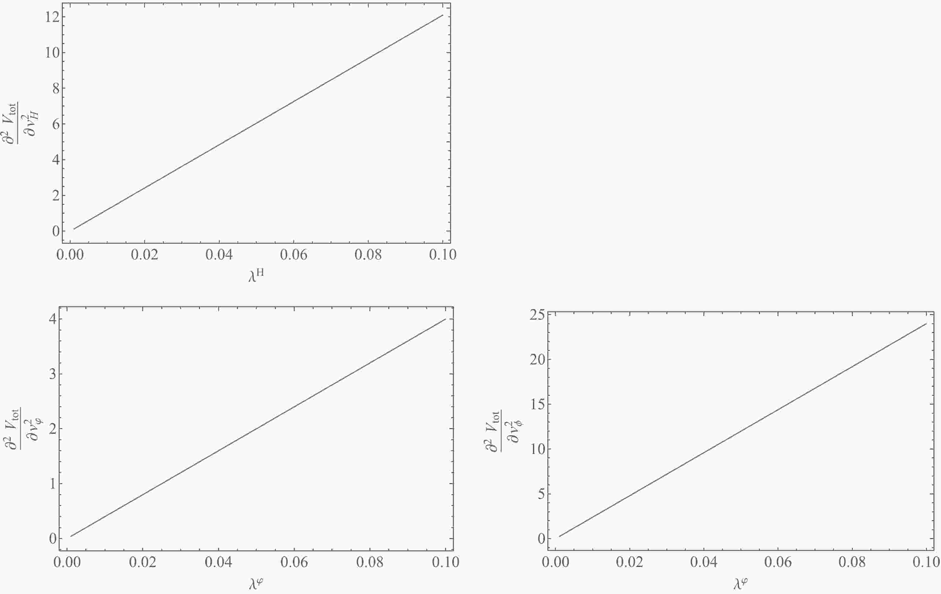
(16) With the help of Eqs. (3) and (16),
$ {\partial^2 V_{\mathrm{tot}}}/{\partial v^2_H} $ depends on$ \lambda^H $ ,$ {\partial^2 V_{\mathrm{tot}}}/{\partial v_{\varphi}^2} $ , and${\partial^2 V_{\mathrm{tot}}}/{\partial v_{\phi}^2}$ depend on$ \lambda^{\varphi} $ , and$ {\partial^2 V_{\mathrm{tot}}}/{\partial v_{\rho}^2} $ and$ {\partial^2 V_{\mathrm{tot}}}/{\partial v_{\eta}^2} $ depend on$ \lambda^{H} $ and$ \lambda^{\rho} $ , which are plotted in Figs. 1 and 2, respectively. These show that the inequalities in (4) are always satisfied by the VEV alignments in (2).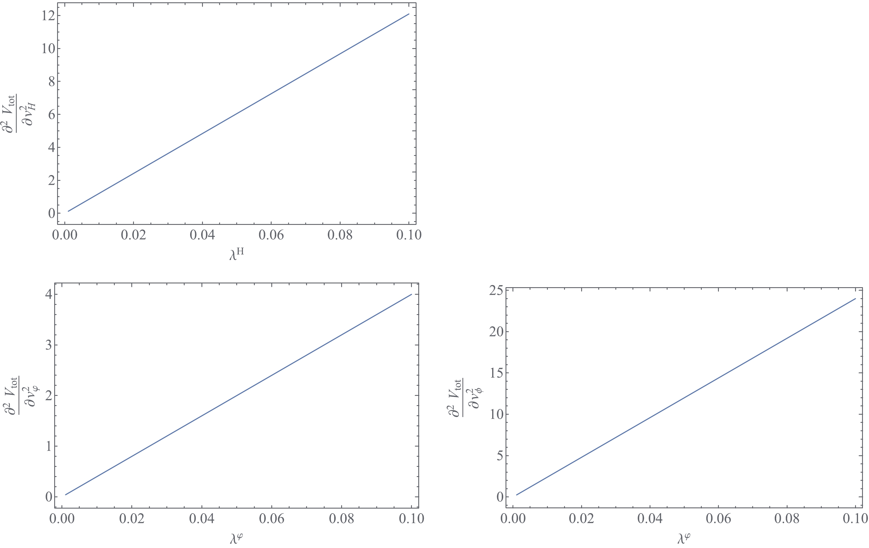
Figure 1. (color online)
$ ({\partial^2 V_{\mathrm{tot}}}/{\partial v^2_H}) \times 10^{-21} $ versus$ \lambda^{H} $ with$ \lambda^{H}\in (10^{-3}, 10^{-1}) $ (upper left),$ ({\partial^2 V_{\mathrm{tot}}}/{\partial v^2_\varphi})\times 10^{-37} $ (bottom left), and$ ({\partial^2 V_{\mathrm{tot}}}/{\partial v^2_\phi})\times 10^{-37} $ (bottom right) versus$ \lambda^{\varphi} $ with$ \lambda^{\varphi}\in (10^{-3}, 10^{-1}) $ 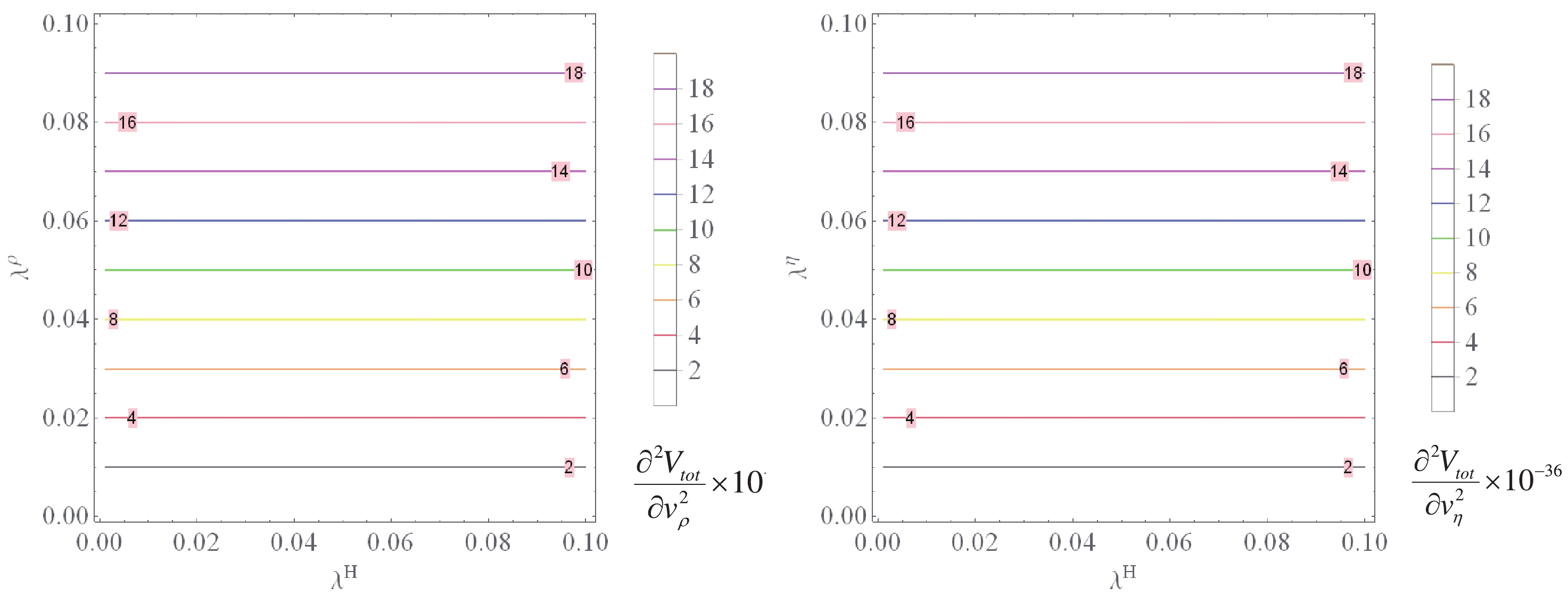
Figure 2. (color online)
$({\partial^2 V_{\mathrm{tot}}}/{\partial v^2_\rho})\times 10^{-36}$ versus$\lambda^{H}$ and$\lambda^{\rho}$ (left panel) and$({\partial^2 V_{\mathrm{tot}}}/{\partial v^2_\eta})\times 10^{-36}$ versus$\lambda^{H}$ and$\lambda^{\eta}$ (right panel) with$\lambda^{H}\in (10^{-3}, 10^{-1})$ ,$\lambda^{\rho} \in (10^{-3}, 10^{-1})$ and$\lambda^{\eta} \in (10^{-3}, 10^{-1})$ . -
Using the tensor product of the
$ T_7 $ group [13, 25], after symmetry breaking, the charged lepton masses and corresponding mixing matrix obtained from the first line of Eq. (1) have the following forms:$ \begin{eqnarray} &&M_{\mathrm{cl}} = \frac{v_H v_\phi}{\Lambda}\left( \begin{array}{ccc} h_1 &\,\,\, h_2 &\,\,\, h_3 \\ h_1 &\,\,\, \omega^2 h_2 &\,\,\, \omega h_3 \\ h_1 &\,\,\, \omega h_2 &\,\,\, \omega^2 h_3\\ \end{array} \right) \quad ( \omega = {\rm e}^{{\rm i}2\pi/3}), \end{eqnarray} $

(17) $ \begin{eqnarray} &&U^+_{\mathrm{L}} = \frac{1}{\sqrt{3}}\left( \begin{array}{ccc} 1 &\,\,\, 1 &\,\,\, 1 \\ 1 &\,\,\, \omega &\,\,\, \omega^2 \\ 1 &\,\,\, \omega^2 &\,\,\, \omega \\ \end{array} \right), \;\;\;U_r = \mathbb{I}_{\mathrm{3\times 3}}. \end{eqnarray} $

(18) Turning now to the neutrino sector. From Eq. (1), when the scalar fields obtain their VEVs, we obtain the following neutrino mass matrices:
$ \begin{eqnarray} m_{\nu N} = x_{1} v_H \mathbb{I}_{\mathrm{3\times 3}} \equiv {\boldsymbol{x}}_1 \mathbb{I}_{\mathrm{3\times 3}}, \;\;\;M_{\nu S} = x_{2} v_H \mathbb{I}_{\mathrm{3\times 3}}\equiv {\boldsymbol{x}}_2 \mathbb{I}_{\mathrm{3\times 3}}, \end{eqnarray} $

(19) $ \begin{eqnarray} m'_{\nu N} = x_3 v_\rho \mathbb{I}_{\mathrm{3\times 3}}\equiv {\boldsymbol{x}}_3\mathbb{I}_{\mathrm{3\times 3}}, \;\;\;M'_{\nu S} = x_4 v_\rho \mathbb{I}_{\mathrm{3\times 3}}\equiv {\boldsymbol{x}}_4 \mathbb{I}_{\mathrm{3\times 3}}, \end{eqnarray} $

(20) $ \begin{eqnarray} M'_{NS}& = & \left( \begin{array}{ccc} y_{1} v_\eta & 0 & y_{3} v^*_\varphi \\ 0 & y_{1} v_\eta &0 \\ y_{2} v_\varphi & 0& y_{1} v_\eta \\ \end{array} \right)\equiv \left( \begin{array}{ccc} {\boldsymbol{y}}_1 & 0 & {\boldsymbol{y}}_3 \\ 0 & {\boldsymbol{y}}_1 & 0 \\ {\boldsymbol{y}}_2 & 0 & {\boldsymbol{y}}_1 \\ \end{array} \right), \end{eqnarray} $

(21) $ \begin{eqnarray} M_{NS} & = &\left( \begin{array}{ccc} z_{1} v_\eta & 0 & z_{3} v^*_\varphi \\ 0 & z_{1} v_\eta &0 \\ z_{2} v_\varphi & 0& z_{1} v_\eta \\ \end{array} \right)\equiv \left( \begin{array}{ccc} {\boldsymbol{z}}_1 & 0 & {\boldsymbol{z}}_3 \\ 0 & {\boldsymbol{z}}_1 & 0 \\ {\boldsymbol{z}}_2 & 0 & {\boldsymbol{z}}_1 \\ \end{array} \right), \end{eqnarray} $

(22) $ \begin{eqnarray} M_{NN}& = &\left( \begin{array}{ccc} t_{1} v_\eta & 0 & t_{3} v^*_\varphi \\ 0 & t_{1} v_\eta &0 \\ t_{2} v_\varphi & 0& t_{1} v_\eta \\ \end{array} \right)\equiv \left( \begin{array}{ccc} {\boldsymbol{t}}_1 & 0 & {\boldsymbol{t}}_3 \\ 0 & {\boldsymbol{t}}_1 & 0 \\ {\boldsymbol{t}}_2 & 0 & {\boldsymbol{t}}_1 \\ \end{array} \right), \end{eqnarray} $

(23) $ \begin{eqnarray} M_{SS}& = &\left( \begin{array}{ccc} g_{1} v_\eta & 0 & g_{3} v^*_\varphi \\ 0 & g_{1} v_\eta &0 \\ g_{2} v_\varphi & 0& g_{1} v_\eta \\ \end{array} \right)\equiv \left( \begin{array}{ccc} {\boldsymbol{g}}_1 & 0 & {\boldsymbol{g}}_3 \\ 0 & {\boldsymbol{g}}_1 & 0 \\ {\boldsymbol{g}}_2 & 0 & {\boldsymbol{g}}_1 \\ \end{array} \right). \end{eqnarray} $

(24) In contrast to the charged lepton sector, all the mass matrices in the neutrino sector are generated from the renormalizable Yukawa terms. The neutrino mass matrix for the linear seesaw, in the
$ \left(\nu_{\rm L}, N_{\rm L}, S_{\rm L}\right) $ ,$ (\nu_{\rm R}, N_{\rm R}, S_{\rm R}) $ basis, takes the form$ \begin{eqnarray} M_{\mathrm{eff}}& = & \left( \begin{array}{ccc} 0& m_{\nu N} & M_{\nu S} \\ m'_{\nu N} & M_{NN} &M_{NS} \\ M'_{\nu S} & M'_{NS} &M_{SS} \\ \end{array} \right)\equiv \left( \begin{array}{ccc} 0&M_\mathrm{D} \\ M{^T_{\mathrm{D}}} & M_{\mathrm{R}} \\ \end{array} \right), \end{eqnarray} $

(25) where
$ \begin{eqnarray} M_\mathrm{D}& = &(m_{\nu N} \,\,\, M_{\nu S}),\;\; M^T_\mathrm{D} = \left( \begin{array}{c} m'_{\nu N}\\ M'_{\nu S} \\ \end{array} \right), \;\; M_\mathrm{R} = \left( \begin{array}{cc} M_{NN} & M_{NS} \\ M'_{NS} & M_{SS} \\ \end{array} \right), \end{eqnarray} $

and all the entries for
$M_{\mathrm{eff}}$ are defined in Eqs. (19)–(24).The light Dirac neutrino mass matrix then gets the form
$ \begin{aligned}[b] M_\nu =& - M_\mathrm{D} M^{-1}_{\mathrm{R}} M^T_\mathrm{D} = -m_{\nu N}M'^{-1}_{NS}M'_{\nu S}-M_{\nu S}M^{-1}_{NS}m'_{\nu N} \\ &- M_{\nu S}M^{-1}_{SS} M'_{\nu S}+m_{\nu N}M^{-1}_{NN}M_{NS}M^{-1}_{SS} M'_{\nu S}\\ &+M_{\nu S}M^{-1}_{SS}M'_{NS}M^{-1}_{NN}m'_{\nu N} +M_{\nu S}M^{-1}_{NS}M_{NN}M'^{-1}_{NS} M'_{\nu S}\\ &-m_{\nu N}M^{-1}_{NN} M_{NS}M^{-1}_{SS}M'_{NS}M^{-1}_{NN}m'_{\nu N}. \end{aligned} $

(26) Combining Eqs. (19)–(24) and (26) yields
$ \begin{eqnarray} M_\nu & = & \left( \begin{array}{ccc} \alpha& 0 & \delta\\ 0& \beta& 0 \\ \kappa & 0 & \gamma \\ \end{array} \right), \end{eqnarray} $

(27) where
$ \begin{eqnarray} \alpha = {\boldsymbol{x}}_1 {\boldsymbol{x}}_{3} \alpha_{13}+{\boldsymbol{x}}_{1} {\boldsymbol{x}}_{4} \alpha_{14} +{\boldsymbol{x}}_{2} {\boldsymbol{x}}_{3} \alpha_{23}+{\boldsymbol{x}}_{2} {\boldsymbol{x}}_{4} \alpha_{24}\equiv \alpha_0 {\rm e}^{{\rm i} \psi_ \alpha}, \end{eqnarray} $

(28) $ \begin{aligned}[b] \beta = &\frac{({\boldsymbol{t}}_{1} {\boldsymbol{x}}_{2}-{\boldsymbol{x}}_{1} {\boldsymbol{z}}_{1}) ({\boldsymbol{x}}_{3} {\boldsymbol{y}}_{1}-{\boldsymbol{t}}_{1} {\boldsymbol{x}}_{4})}{{\boldsymbol{g}}_{1} {\boldsymbol{t}}_{1}^2} \\& +\frac{{\boldsymbol{t}}_{1} {\boldsymbol{x}}_{2} {\boldsymbol{x}}_{4}-{\boldsymbol{x}}_{1} {\boldsymbol{x}}_{4} {\boldsymbol{z}}_{1}-{\boldsymbol{x}}_{2} {\boldsymbol{x}}_{3} {\boldsymbol{y}}_{1}}{{\boldsymbol{y}}_{1} {\boldsymbol{z}}_{1}}\equiv \beta_0 {\rm e}^{{\rm i} \psi_\beta}, \end{aligned} $

(29) $ \gamma = {\boldsymbol{x}}_1 {\boldsymbol{x}}_{3}\gamma_{13} + {\boldsymbol{x}}_{1} {\boldsymbol{x}}_{4} \gamma_{14} +{\boldsymbol{x}}_{2} {\boldsymbol{x}}_{3} \gamma_{23} + {\boldsymbol{x}}_{2} {\boldsymbol{x}}_{4} \gamma_{24} \equiv \gamma_0 {\rm e}^{{\rm i} \psi_\gamma}, $

(30) $ \delta = {\boldsymbol{x}}_1 {\boldsymbol{x}}_{3}\delta_{13}+{\boldsymbol{x}}_{1} {\boldsymbol{x}}_{4}\delta_{14} + {\boldsymbol{x}}_{2} {\boldsymbol{x}}_{3} \delta_{23}+ {\boldsymbol{x}}_{2} {\boldsymbol{x}}_{4}\delta_{24}\equiv \delta_0 {\rm e}^{{\rm i} \psi_\delta}, $

(31) $ \kappa = {\boldsymbol{x}}_1 {\boldsymbol{x}}_{3} \kappa_{13}+ {\boldsymbol{x}}_{1} {\boldsymbol{x}}_{4}\kappa_{14} +{\boldsymbol{x}}_{2} {\boldsymbol{x}}_{3} \kappa_{23}+ {\boldsymbol{x}}_{2} {\boldsymbol{x}}_{4}\kappa_{24}\equiv \kappa_0 {\rm e}^{{\rm i} \psi_\kappa}, $

(32) with
$ \alpha_{mn}, \gamma_{mn}, \delta_{mn} $ , and$ \kappa_{mn}\, (mn = 13, 14, 23, 24) $ given in Appendix D.First, we define the Hermitian matrix
$M^2_\nu $ given by$ \begin{eqnarray} M^2_\nu& = &M_{\nu} M^+_{\nu} = \left( \begin{array}{ccc} a_0^2 & 0 & d_{0} {\rm e}^{{\rm i} \Psi} \\ 0 & \beta_{0}^2 & 0 \\ d_{0} {\rm e}^{-{\rm i} \Psi} & 0 &c^2_0 \\ \end{array} \right), \end{eqnarray} $

(33) where
$ \begin{eqnarray} &&a_0^2 = \alpha^2_0 + \delta^2_0, c_0^2 = \gamma^2_0 + \kappa^2_0, \end{eqnarray} $

(34) $ \begin{eqnarray} &&d_0 {\rm e}^{{\rm i}\psi} = \gamma_0 \delta_0 {\rm e}^{-{\rm i} (\psi_\gamma-\psi_\delta)}+ \alpha_0 \kappa_0 {\rm e}^{{\rm i} (\psi_\alpha-\psi_\kappa)}. \end{eqnarray} $

(35) The mass matrix
$ M^2_\nu $ is diagonalized by$U_{\nu } $ satisfying$ \begin{eqnarray}\\[-5pt] U_{\nu }^+ M^2_\nu U_{\nu } = \left\{ \begin{array}{l} \left( \begin{array}{ccc} m^2_1 & 0 & 0 \\ 0 & m^2_{2} & 0 \\ 0 & 0 & m^2_{3} \end{array} \right) ,\;\; U_{\nu } = \left( \begin{array}{ccc} \cos \theta & 0 & -\sin\theta .{\rm e}^{{\rm i} \Psi}\\ 0 & 1 & 0 \\ \sin\theta .{\rm {\rm e}}^{-{\rm i} \Psi} & 0 & \cos \theta \\ \end{array} \right) \;\rm{for NO,}\ \ \\ \left( \begin{array}{ccc} m^2_{3} & 0 & 0 \\ 0 & m^2_{2} & 0 \\ 0 & 0 & m^2_1 \end{array} \right) ,\;\;U_{\nu } = \left( \begin{array}{ccc} \sin\theta & 0 &\cos \theta {\rm e}^{{\rm i} \Psi}\\ 0 & 1 & 0 \\ -\cos \theta {\rm e}^{-{\rm i} \Psi} & 0 &\sin\theta \\ \end{array} \right) \;\rm{for IO, } \end{array} \right.\end{eqnarray} $ 
(36) where
$ \begin{eqnarray} m^2_1 = \beta_0^2 - \Delta m^2_{21}, \quad m^2_2 = \beta_0^2, \quad m^2_3 = \beta_0^2+ \Delta m^2_{31}- \Delta m^2_{21}. \end{eqnarray} $

(37) The sum of neutrino masses is given by
$ \begin{eqnarray} \sum m_\nu = \beta_0+\sqrt{\beta_0^2-\Delta m^2_{21}}+\sqrt{\beta_0^2-\Delta m^2_{21}+\Delta m^2_{31}}. \end{eqnarray} $

(38) Using the expressions for
$ U_{\mathrm{Lep}} $ and$U_{\nu } $ in Eqs. (18) and (36), the leptonic mixing matrix,$ U_{\mathrm{Lep}} = U_{\mathrm{L}}^{+} U_{\nu } $ , is given by$ \begin{eqnarray} U_{\mathrm{Lep}} = \left\{ \begin{array}{l} \dfrac{1}{\sqrt{3}}\left( \begin{array}{ccc} \cos\theta + \sin\theta. {\rm e}^{-{\rm i} \Psi } &1 & \cos\theta - \sin\theta. {\rm e}^{{\rm i} \Psi} \\ \cos\theta + \omega^2 \sin\theta. {\rm e}^{-{\rm i} \Psi} & \omega & \omega^2\cos\theta - \sin\theta. {\rm e}^{{\rm i} \Psi} \\ \cos\theta + \omega \sin\theta. {\rm e}^{-{\rm i} \Psi}& \omega^2 & \omega \cos\theta - \sin\theta. {\rm e}^{{\rm i} \Psi} \\ \end{array}\right) \;\rm{for NO}, \\ \dfrac{1}{\sqrt{3}}\left( \begin{array}{ccc} \sin\theta-\cos\theta. {\rm e}^{-{\rm i} \Psi } &1 & \sin\theta+\cos\theta. {\rm e}^{{\rm i} \Psi} \\ \sin\theta - \omega^2 \cos\theta. {\rm e}^{-{\rm i} \Psi} & \omega & \omega^2\sin\theta +\cos\theta. {\rm e}^{{\rm i} \Psi} \\ \sin\theta - \omega \cos\theta. {\rm e}^{-{\rm i} \Psi}& \omega^2 & \omega \sin\theta+\cos\theta. {\rm e}^{{\rm i} \Psi} \\ \end{array}\right) \;\rm{for IO}. \end{array} \right. \end{eqnarray} $

(39) Expression (39) implies that
$ U_{\mathrm{Lep}} $ possesses the$ \mathrm{TM}_2 $ form because$ \left(U_{\mathrm{Lep}}\right)_{i2} = \dfrac{1}{\sqrt{3}}\, (i = 1,2,3) $ .Now, comparing Eq. (39) with the standard parameterization of
$ U_{\rm PMNS} $ [24], we can parameterize the solar neutrino mixing angle$ \theta_{12} $ , Dirac CP phase$ \delta_{\rm CP} $ , and model parameters$ \theta, \;\Psi,\; \eta_1 $ in terms of the other two neutrino mixing angles$ \theta_{13} $ and$ \theta_{23} $ , as follows②:$ \begin{eqnarray} &&s^2_{12} = \frac{1}{3c^2_{13}} \;\rm{for both NO and IO}, \end{eqnarray} $

(40) $ \begin{eqnarray} &&s_\theta = \left\{ \begin{array}{l} \sqrt{\dfrac{1}{2} +\dfrac{\sqrt{3}}{2}\sqrt{c^4_{13} s'^2_{23}-c'^2_{13}}} \;\;\rm{for NO}, \\ \sqrt{\dfrac{1}{2} - \dfrac{\sqrt{3}}{2}\sqrt{c^4_{13} s'^2_{23}-c'^2_{13}}}\,\;\rm{for IO}, \end{array} \right. \end{eqnarray} $

(41) $ \begin{eqnarray} && \sin\delta_{\rm CP} = -\frac{\sqrt{c^4_{13} s'_{23}-c'^2_{13}}}{s'_{23} s_{13} \sqrt{2-3 s^2_{13}}} \;\rm{for both NO and IO}, \end{eqnarray} $

(42) $ \begin{eqnarray} &&\Psi = \left\{ \begin{array}{l} -\sec ^{-1}\left(\dfrac{\sqrt{4-3(s'^2_{13}+4 c_{13}^4 s'^2_{23})}}{1-3 s_{13}^2}\right) \,\;\rm{for NO}, \\ -\sec ^{-1}\left(\dfrac{\sqrt{4-3(s'^2_{13}+4 c_{13}^4 s'^2_{23})}}{3 s_{13}^2-1}\right) \,\;\rm{for IO}, \end{array} \right. \end{eqnarray} $

(43) $ \begin{eqnarray} &&\eta_1 = \left\{ \begin{array}{l} -{\rm i} \log \left(\dfrac{c_\theta+s_\theta {\rm e}^{-{\rm i} \Psi}}{\sqrt{3} c_{12} c_{13}}\right) \,\;\rm{for NO}, \\ \dfrac{\rm i}{2} \log (3)-{\rm i} \log \left(\dfrac{s_\theta-c_\theta {\rm e}^{-{\rm i} \Psi}}{c_{12} c_{13}}\right)\,\;\rm{for IO}, \end{array} \right. \end{eqnarray} $

(44) $ \begin{eqnarray} &&\eta_2 = 0\; \rm{for both NO and IO} . \end{eqnarray} $

(45) -
The considered model contains three degrees of freedom in the neutrino sector corresponding to three free parameters, including
$ \beta_0,\; \theta $ , and Ψ. In the three neutrino framework, there are eight independent parameters in total, including two neutrino squared mass splittings,$ \Delta m^2_{21} $ and$ \Delta m^2_{31} $ , for NO ($ \Delta m^2_{32} $ for IO), three mixing angles ($ \theta_{12}, \theta_{13}, \theta_{23} $ ), one CP phase ($ \delta_{\rm CP} $ ), and two Majorana phases ($ \eta_{1}, \eta_{2} $ ) in which$ \eta_{1}, \;\eta_{2} $ are currently undetermined while the others can be exactly observed. As shown in Table 1, five observable quantities$ \theta_{12},\; \theta_{13},\; \theta_{23} $ ,$ \Delta m^2_{21} $ , and$ \Delta m^2_{31} $ for NO ($ \Delta m^2_{32} $ for IO) are more precisely determined, whereas$ \delta_{\rm CP} $ is less precise.First, Eq. (37) shows that
$ m_{1,2,3} $ depend on two observed parameters,$ \Delta m^2_{21} $ and$ \Delta m^2_{31} $ , which have been determined with high accuracy, and one model parameter,$ \beta_0 $ , which is of the same order of magnitude as the second neutrino mass$ m_2 $ . The neutrino mass scale is unknown; however, from Eq. (38), we can estimate the allowed regions for$ \beta_0 $ using the upper limits of$ \sum m_\nu $ with$ \sum m_\nu < 120\,\; \mathrm{meV} $ for NO,$ \sum m_\nu < 150\,\; \mathrm{meV} $ for IO [1], and the best fit values of$ \Delta m^2_{21} $ and$ \Delta m^2_{31} $ taken from [1] with$ \Delta m^2_{21} = 75 \,\;\mathrm{meV}^2 $ and$ \Delta m^2_{31} = 2.55\times 10^3 \,\;\mathrm{meV}^2 $ for NO and$ \Delta m^2_{31} = -2.45\times10^3 \,\;\mathrm{meV}^2 $ for IO. From this, we obtain the allowed range of$ \beta_0 $ .$ \begin{eqnarray} &&\beta_0\in \left\{ \begin{array}{l} (10,\, 30)\,\; \mathrm{meV} \;\rm{for NO}, \\ (51, 60) \,\; \mathrm{meV} \;\rm{for IH}. \end{array} \right. \end{eqnarray} $

(46) The estimation of
$ \beta_0 $ allows us to predict neutrino masses. Figure 3 shows the allowed neutrino mass regions as a function of$ \beta_0 $ , which are estimated to be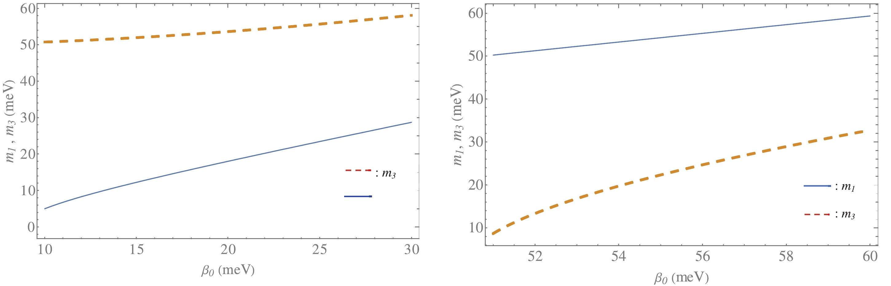
Figure 3. (color online)
$ m_{1} $ and$ m_{3} $ versus$ \beta_{0}\equiv m_{2} $ with$ \beta_{0}\in (10.0, 30.0)\,\; \mathrm{meV} $ for NO (left panel) and$ \beta_{0}\in (50.0, 60.0)\,\; \mathrm{meV} $ for IO (right panel).$ \begin{eqnarray} &&\left\{ \begin{array}{l} m_1\in (5.0, 28.0)\,\; \mathrm{meV}, \;\;m_3 = (51.0, 58.0) \,\; \mathrm{meV} \;\rm{for NO}, \\ m_1\in (50.5, 59.3)\,\; \mathrm{meV},\,\; m_3 = (8.7, 32.8) \,\; \mathrm{meV} \;\rm{for IO}. \end{array} \right. \end{eqnarray} $

(47) We now return to the lepton mixing sector. The global reassessment of neutrino oscillation [1] reveals that in the
$ 3\, \sigma $ range of the best-fit value,$ s^2_{13}\in (0.02, 0.02405) $ ; thus, using Eq. (40), we can estimate the allowed regions of$ s^2_{12} $ .$ \begin{aligned}[b]& s^2_{12} \in (0.3402, 0.3416), \,\, \mathrm{i.e.},\,\,\\& \theta_{12} (^\circ) \in (35.677, 35.762). \end{aligned} $

(48) Using Eq. (4) and
$ 3\sigma $ ranges for$ \sin\theta_{13} $ and$ \theta_{23} $ , we plot in Fig. 4 the relationship between$ \sin\theta $ and$ \theta_{13}, \;\theta_{23} $ and obtain the allowed regions of$ \sin\theta $ .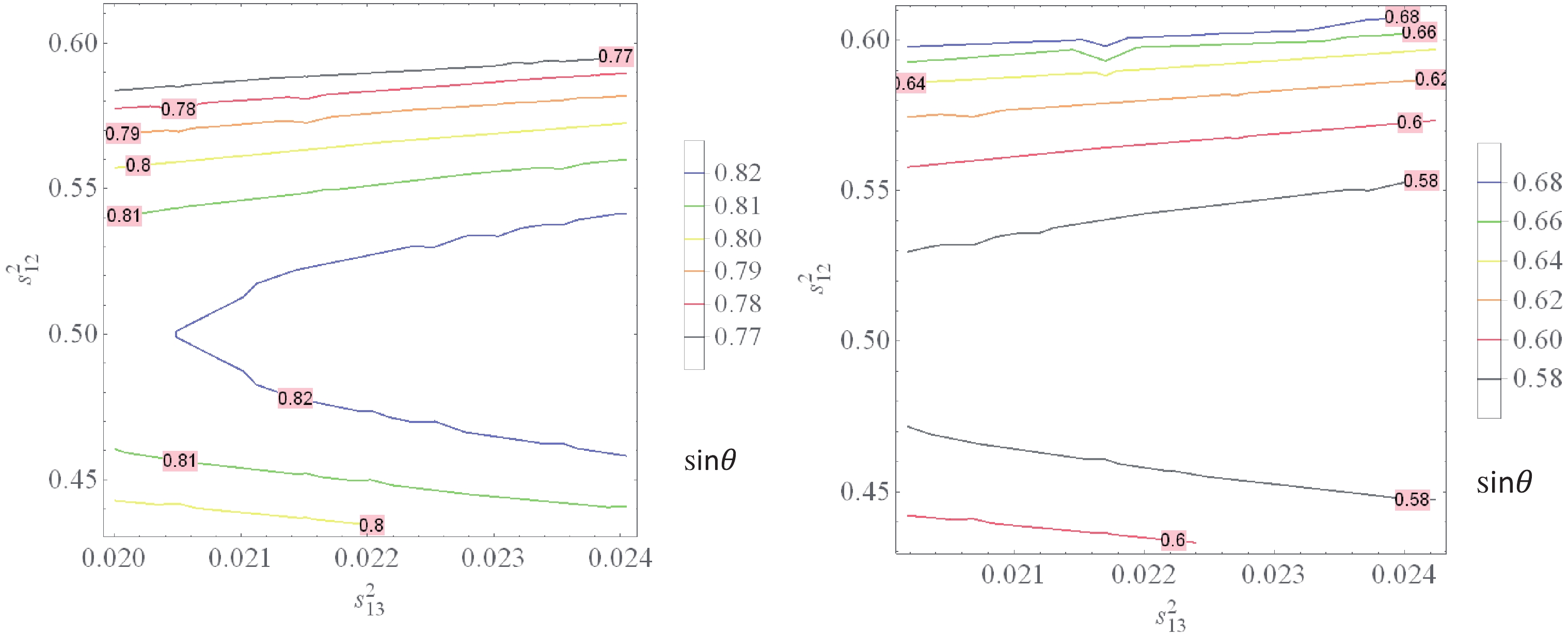
Figure 4. (color online)
$ s_\theta $ versus$ s^2_{13} $ and$ s^2_{23} $ with$ s^2_{13}\in (2.000, 2.405)\times 10^{-2} $ and$ s^2_{23} \in (0.434, 0.610) $ for NH (left panel) while$ s^2_{13}\in (2.018, 2.424)\times 10^{-2} $ and$ s^2_{23} \in (0.433, 0.608) $ for IH (right panel).$ \begin{aligned}[b]& s_\theta \in \left\{ \begin{array}{l} (0.77, 0.82) \;\rm{for NO}, \\ (0.58, 0.68) \;\rm{for IO}, \end{array} \right. \,\, \mathrm{i.e.},\,\, \\&\theta (^\circ) \in \left\{ \begin{array}{l} (50.35, 55.08) \;\rm{for NO}, \\ (35.45, 42.84)\; \rm{for IO}. \end{array} \right. \end{aligned} $

(49) Next, in Fig. 5, we plot the relationship between
$ \sin\delta_{\rm CP} $ and$ \theta_{13},\; \theta_{23} $ based on Eq. (42) and predict the allowed regions of$ \sin\delta_{\rm CP} $ as follows: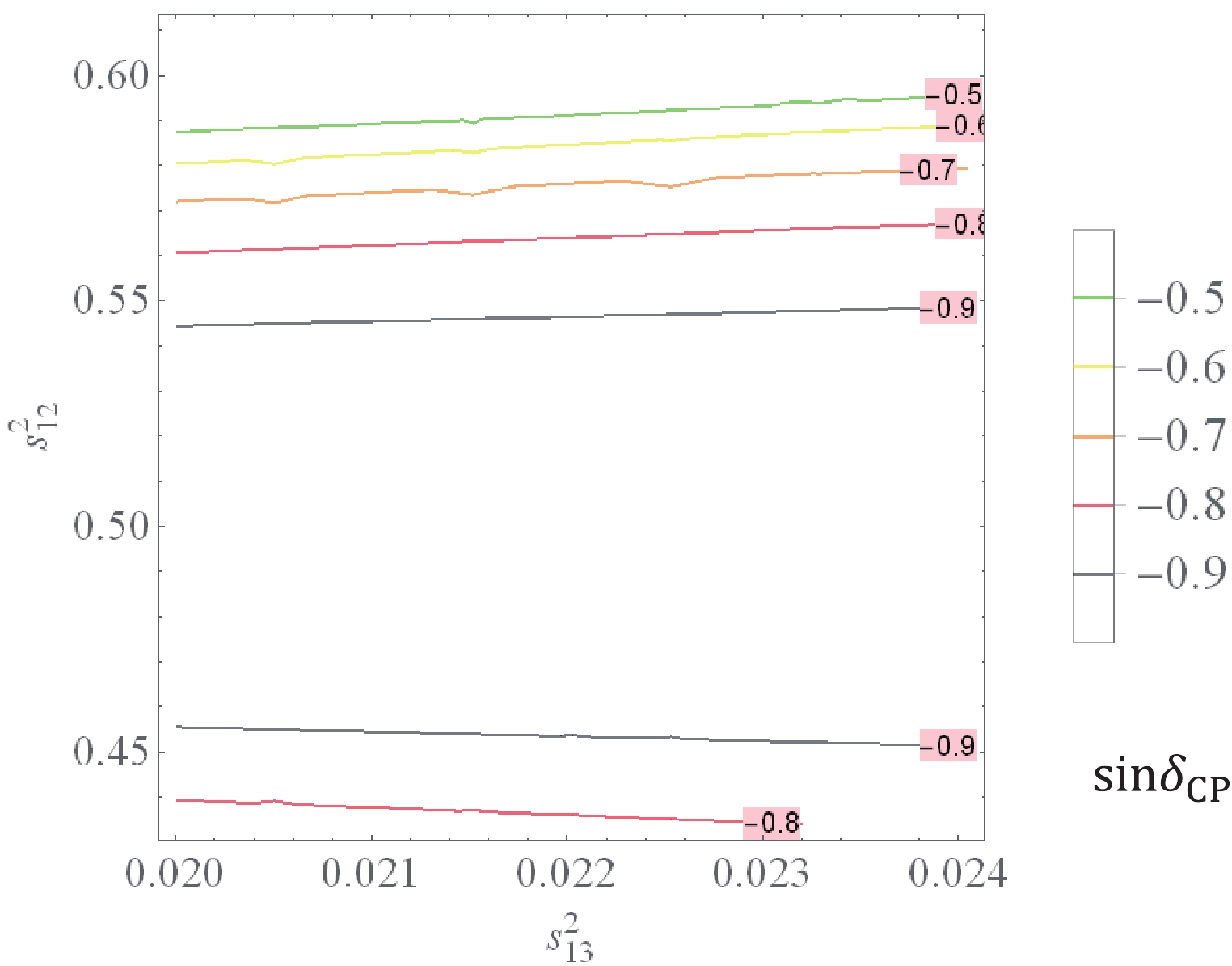
Figure 5. (color online)
$\sin\delta_{\rm CP}$ versus$ s^2_{13} $ and$ s^2_{23} $ with$ s^2_{13}\in $ $ (2.000, 2.405)\times 10^{-2} $ and$ s^2_{23} \in (0.434, 0.610) $ .$ \begin{eqnarray} \sin \delta_{\rm CP} \in (-0.90, -0.50), \,\, \mathrm{i.e.},\,\, \delta_{\rm CP} (^\circ) \in (295.80,330.0). \end{eqnarray} $

(50) This value of
$ \delta_{\rm CP} $ lies in the$ 3\sigma $ ranges taken from Ref. [1] for both NO and IO.Similarly, from Eq. (43), we plot the correlation between the model parameter Ψ and
$ \theta_{13},\; \theta_{23} $ , as in Fig. 6. This figure indicates that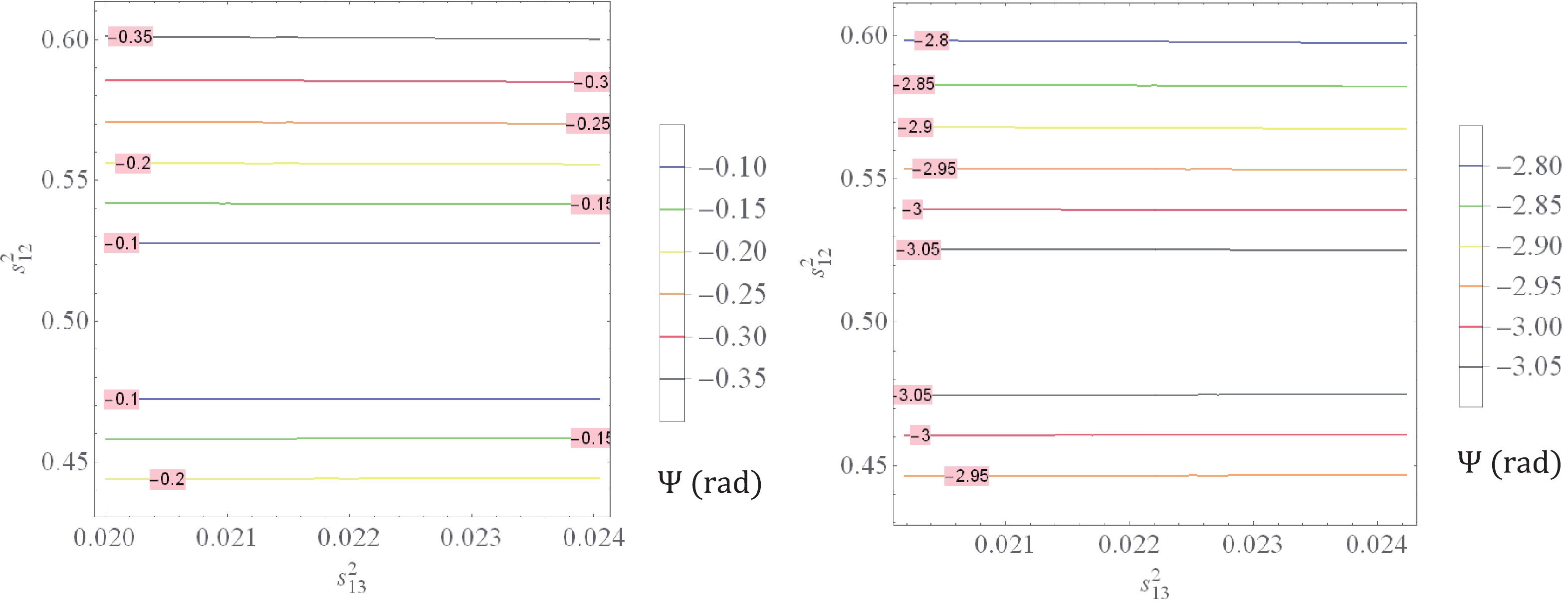
Figure 6. (color online)
$ \Psi\, (\mathrm{rad}) $ versus$ s^2_{13} $ and$ s^2_{23} $ with$ s^2_{13}\in (2.000, 2.405)\times 10^{-2} $ and$ s^2_{23} \in (0.434, 0.610) $ for NH (left panel) while$ s^2_{13}\in (2.018, 2.424)\times 10^{-2} $ and$ s^2_{23} \in (0.433, 0.608) $ for IH (right panel).$ \begin{eqnarray} \Psi(^\circ) \in \left\{ \begin{array}{l} (5.73, 20.05) \;\rm{for NO}, \\ (185.20,199.60) \;\rm{for IO}. \end{array} \right. \end{eqnarray} $

(51) In our model, one Majorana phase is predicted to be zero
$ (\eta_2 = 0) $ for both mass orderings, and the other ($ \eta_1 $ ) is predicted to be$ \begin{eqnarray} \eta_1(^\circ) \in \left\{ \begin{array}{l} (3.44, 10.37) \;\rm{for NO}, \\ (349.60,356.60) \;\rm{for IO}, \end{array} \right. \end{eqnarray} $

(52) as shown in Fig. 7.
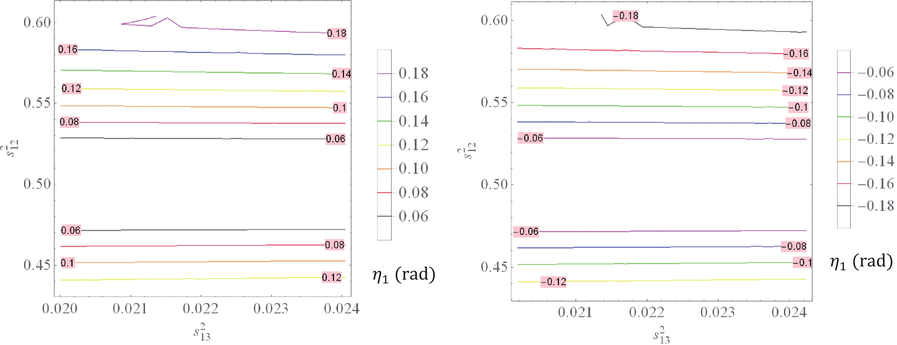
Figure 7. (color online)
$ \eta_1\, (\mathrm{rad}) $ versus$ s^2_{13} $ and$ s^2_{23} $ with$ s^2_{13}\in (2.000, 2.405)\times 10^{-2} $ and$ s^2_{23} \in (0.434, 0.610) $ for NH (left panel) while$ s^2_{13}\in (2.018, 2.424)\times 10^{-2} $ and$ s^2_{23} \in (0.433, 0.608) $ for IH (right panel).As an example, at the best-fit points of
$ s^2_{13} $ and$ s^2_{23} $ given in Table 1,$ s^2_{13} = 2.20\times 10^{-2}, \;s^2_{23} = 0.574 $ for NO and$ s^2_{13} = 2.225\times 10^{-2}, \;s^2_{23} = 0.578 $ for IO; hence, we obtain$ \begin{eqnarray} &&s^2_{12} = \left\{ \begin{array}{l} 0.3408 \;\rm{for NO}, \\ 0.3409 \;\rm{for IO}, \end{array} \right.\;\; \theta_{12} = \left\{ \begin{array}{l} 35.72^\circ \;\rm{for NO}, \\ 35.72^\circ \;\rm{for IO}, \end{array} \right. \end{eqnarray} $

(53) $ \begin{eqnarray} &&s_{\theta} = \left\{ \begin{array}{l} 0.792 \;\rm{for NO}, \\ 0.6151 \;\rm{for IO}, \end{array} \right. \;\;\theta = \left\{ \begin{array}{l} 52.37^\circ \;\rm{for NO}, \\ 37.96^\circ \;\rm{for IO}, \end{array} \right. \end{eqnarray} $

(54) $ \begin{eqnarray} &&\sin \delta_{\rm CP} = \left\{ \begin{array}{l} -0.7204 \;\rm{for NO}, \\ -0.686 \;\rm{for IO}, \end{array} \right. \;\;\delta_{\rm CP} = \left\{ \begin{array}{l} 313.90^\circ \;\rm{for NO}, \\ 316.70^\circ \;\rm{for IO}, \end{array} \right. \end{eqnarray} $

(55) $ \begin{eqnarray} &&\Psi = \left\{ \begin{array}{l} 345.00^\circ \;\rm{for NO}, \\ 195.80^\circ \;\rm{for IO}, \end{array} \right. \;\; \eta_1 = \left\{ \begin{array}{l} 8.49^\circ \;\rm{for NO}, \\ 351.10^\circ \;\rm{for IO}. \end{array} \right. \end{eqnarray} $

(56) The unitary lepton mixing matrix becomes
$\begin{aligned}[b] U_{\mathrm{Lep}}=\left\{ \begin{aligned} \left( \begin{array}{ccc} 0.7941\, +0.1185 {\rm i} & 0.5774 & -0.08915+0.1185 {\rm i} \\ 0.2343\, -0.4417 {\rm i} & -0.2887+0.5000 {\rm i} & -0.6179-0.1867 {\rm i} \\ 0.0290\, +0.3232 {\rm i} & -0.2887-0.5000 {\rm i} & -0.6179+0.4238 {\rm i} \\ \end{array} \right) \hspace{0.1cm}\;\rm{for NO}, \\ \left( \begin{array}{ccc} 0.7931\, -0.1240 {\rm i} & 0.5774 & -0.08292-0.1240 {\rm i} \\ 0.0287\, -0.3173{\rm i} & -0.2887+0.5000 {\rm i} & -0.6156-0.4315 {\rm i} \\ 0.2435\, +0.4413 {\rm i} & -0.2887-0.5000 {\rm i} & -0.6156+0.1835 {\rm i} \\ \end{array} \right) \;\hspace{0.1cm}\rm{for IO}, \end{aligned} \right.\end{aligned}$

(57) which are all consistent with the entry constraints given in Ref. [26].
-
We now deal with the effective neutrino masses related to beta decay and neutrinoless double beta decay, which have the following respective forms [27–29]:
$\begin{aligned}[b] m_{\beta } = & \sqrt{\sum^3_{k = 1} \left|U_{1 k}\right|^2 m_k^2} = \sqrt{\beta_0^2 - \frac{2}{3} \Delta m^2_{21}+ \Delta m^2_{31} s^2_{13}} \;\\&\rm{for\; both \;orderings,} \end{aligned} $

(58) $ \begin{eqnarray} &&\langle m_{ee}\rangle = \left| \sum^3_{k = 1} U_{1 k}^2 m_k \right| = \left\{ \begin{array}{l} \dfrac{\sqrt{\beta_N}}{3} \;\rm{for NO,} \\ \dfrac{\sqrt{\beta_I}}{3} \;\rm{for IO,} \end{array} \right. \end{eqnarray} $

(59) where
$ \beta_N $ and$ \beta_I $ are given in Appendix E. Expressions (58), (59), and (E1)–(E3) reveal that$ \langle m_{ee}\rangle $ depends on five parameters$ \theta_{12}, \theta_{23} $ ,$ \Delta m^2_{21} $ ,$ \Delta m^2_{31} $ , and$ \beta_0 $ , whereas$ m_{\beta } $ depends on four parameters$ \theta_{12} $ ,$ \Delta m^2_{21} $ ,$ \Delta m^2_{31} $ , and$ \beta_0 $ . At the best-fit points of$ \Delta m^2_{21} $ and$ \Delta m^2_{31} $ taken from Table 1,$ \beta_0 $ is fixed at$ \beta_0 = 20.0 \,\; \mathrm{meV} $ for NO and$ \beta_0 = 55.0\,\; \mathrm{meV} $ for IO, and$ \langle m_{ee}\rangle $ depends on$ s^2_{13} $ and$ s^2_{23} $ , whereas$ m_{\beta } $ depends only on$ s^2_{13} $ , which are plotted in Figs. 8 and 9, respectively. These imply that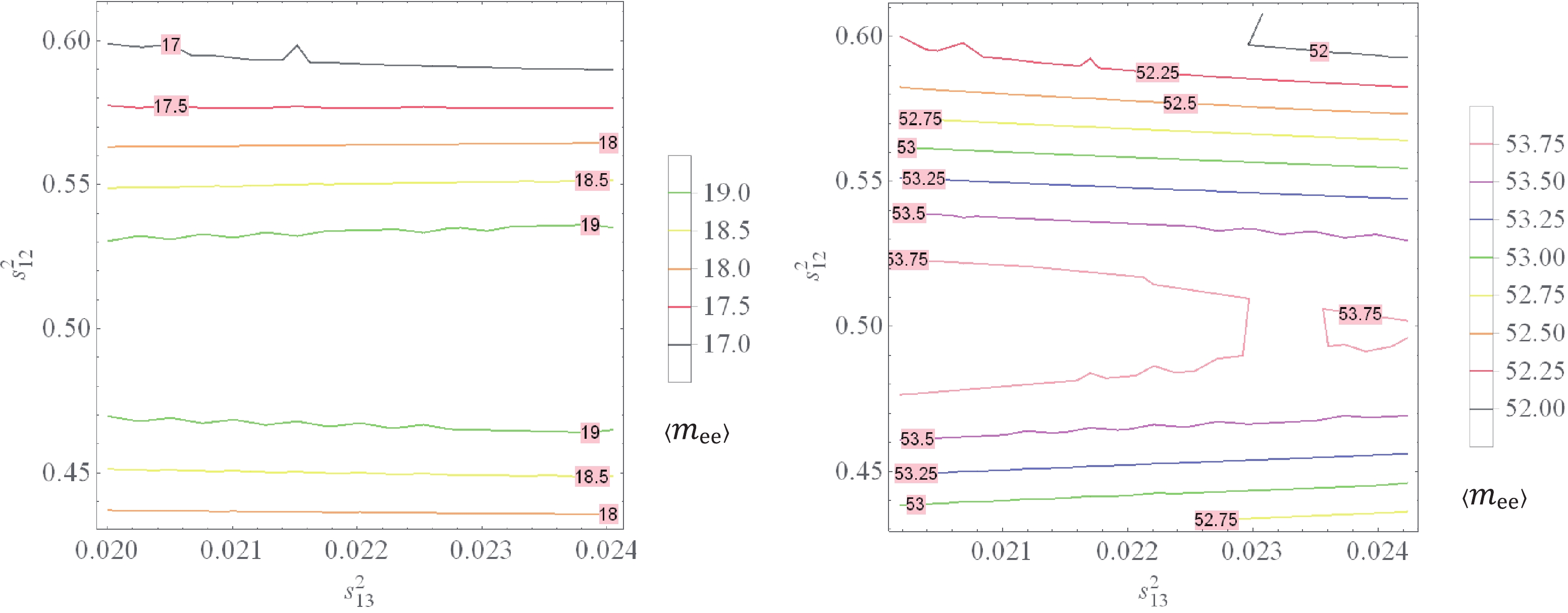
Figure 8. (color online)
$ \langle m_{ee}\rangle $ (in meV) versus$ s^2_{13} $ and$ s^2_{23} $ with$ s^2_{13}\in (2.000, 2.405)\times 10^{-2} $ and$ s^2_{23} \in (0.434, 0.610) $ for NH (left panel) while$ s^2_{13}\in (2.018, 2.424)\times 10^{-2} $ and$ s^2_{23} \in (0.433, 0.608) $ for IH (right panel).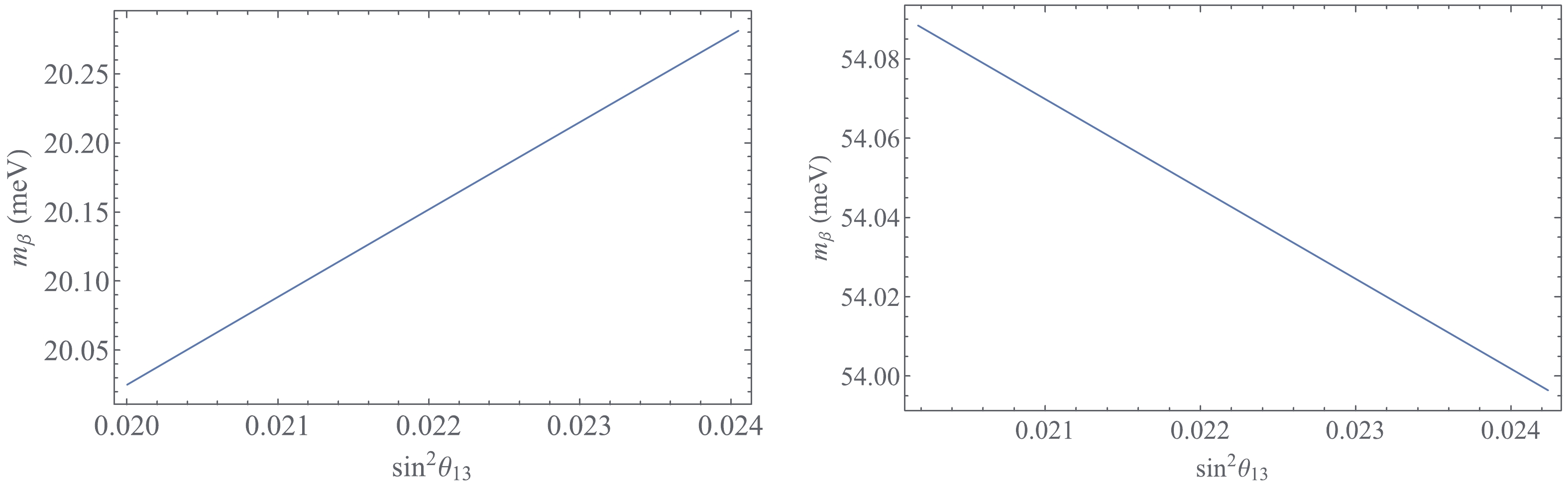
Figure 9. (color online)
$ m_\beta $ (in meV) versus$ s^2_{13} $ with$ s^2_{13}\in (2.000, 2.405)\times 10^{-2} $ for NH (left panel) and$ s^2_{13}\in (2.018, 2.424)\times 10^{-2} $ for IH (right panel).$ \begin{eqnarray} &&\langle m_{ee}\rangle \in \left\{ \begin{array}{l} (47.00, 50.50) \; \rm{meV}^2 \;\rm{for NO,} \\ (48.40, 49.40) \; \rm{meV} \;\rm{for IO,} \end{array} \right. \end{eqnarray} $

(60) $ \begin{eqnarray} && m_{\beta} \in\left\{ \begin{array}{l} (51.02, 51.10)\; \rm{meV} \;\rm{for NO,} \\ (49.92, 50.02)\; \rm{meV} \;\rm{for IO}. \end{array} \right. \end{eqnarray} $

(61) At the best-fit points of
$ s^2_{13} $ and$ s^2_{23} $ taken from Table 1,$ s^2_{13} = 2.20\times 10^{-2} $ and$ s^2_{23} = 0.574 $ for NO while$s_{13}^2 = $ $ 2.225\times 10^{-2},\; s_{23}^2 = 0.578$ for NO; hence, we obtain$ \begin{eqnarray} &&\langle m_{ee}\rangle = \left\{ \begin{array}{l} 17.60\; \mathrm{meV} \;\rm{for NO}, \\ 48.74 \; \mathrm{meV} \;\rm{for IO}, \end{array} \right. \end{eqnarray} $

(62) $ \begin{eqnarray} &&m_\beta = \left\{ \begin{array}{l} 20.15\, \mathrm{meV} \;\rm{for NO}, \\ 49.96\, \mathrm{meV} \;\rm{for IO}, \end{array} \right. \end{eqnarray} $

(63) provided that
$ \beta_0 = 20.0 \,\; \mathrm{meV} $ for NO and$ \beta_0 = 55.0\,\; \mathrm{meV} $ for IO.The predicted ranges of
$ m_{\beta } $ and$ \langle m_{ee}\rangle $ in Eqs. (60) and (61) for both orderings satisfy all the upper bounds taken from recent$ 0\nu \beta \beta $ decay experiments, such as the PLANCK Collaboration$ \langle m_{ee} \rangle < 80 \div 180 \,\;\mathrm{meV} $ [30, 31], CUORE Collaboration [32]$ \langle m_{ee} \rangle < 75 \div 350 \,\;\mathrm{meV} $ , and GERDA Collaboration [33]$ \langle m_{ee} \rangle < 70 \div 160 \,\;\mathrm{meV} $ . -
We propose a low-scale Standard Model extension with
$ T_7\times Z_4 \times Z_3\times Z_2 $ symmetry that can successfully explain the observed neutrino oscillation results within the$ 3 \sigma $ range. The small neutrino masses are obtained via the linear seesaw mechanism. Normal and inverted neutrino mass orderings are considered with three lepton mixing angles in their allowed 3$ \sigma $ ranges. The prediction for the Dirac phase is$ \delta_{\rm CP}\in (295.80,\,330.0)^\circ $ for both normal and inverted orderings, including its experimentally maximum value, while those for the two Majorana phases are$ \eta_1\in (349.60,\,356.60)^\circ,\, \eta_2 = 0 $ for normal ordering and$ \eta_1\in (3.44,\, 10.37)^\circ, \,\; \eta_2 = 0 $ for inverted ordering. In addition, the predictions for the effective neutrino masses are$ \langle m_{ee}\rangle \in (47.00,\, 50.50) \, \;\rm{meV}, $ $ m_{\beta} \in (51.02, $ $ \,51.10)\,\; \rm{meV} $ for normal ordering and$ \langle m_{ee}\rangle \in $ $ (48.40, \, $ $ 49.40) \, \;\rm{meV},\, \;m_{\beta} \in (49.92, \,50.02)\; \rm{meV} $ for inverted ordering, which are consistent with the present experimental bounds. -
The Frobenius group
$ T_7 $ is isomorphic to$ Z_7 \rtimes Z_3 $ and has 21 elements divided into five conjugacy classes corresponding to its five irreducible representations, including three singlets,$ {\bf{1}}_{0},\, {\bf{1}}_{1}, \, {\bf{1}}_{2} $ , and two triplets,$ {\bf{3}}, \, {\bar{\bf{3}}} $ . All the group multiplication rules of$ T_7 $ as given below.The tensor products between singlets of
$ T_7 $ are [13, 25]$ \begin{aligned}[b]\\[-7pt] &{\bf{1}}_0 (a) \otimes {\bf{1}}_k (b) = {\bf{1}}_k(ab) (k = 1, 2), \\ &{\bf{1}}_0 (a) \otimes {\bf{1}}_0 (b) = {\bf{1}}_1 (a) \otimes {\bf{1}}_2 (b) = {\bf{1}}_2 (a) \otimes {\bf{1}}_1 (b) = {\bf{1}}_0 (ab), \\ &{\bf{1}}_1 (a) \otimes {\bf{1}}_1 (b) = {\bf{1}}_2(ab), \,\, {\bf{1}}_2 (a) \otimes {\bf{1}}_2 (b) = {\bf{1}}_1(ab). \end{aligned}\tag{A1} $ 
The tensor products between singlets and triplets of
$ T_7 $ are [13, 25]$ \begin{aligned}[b] {\bf{1}}_0 (a) \otimes {\bf{3}} (b_1, b_2, b_3) =& {\bf{3}} (ab_1, ab_2, ab_3), \,\, {\bf{1}}_1 (a)\otimes {\bf{3}} (b_1, b_2, b_3) = {\bf{3}}(ab_1, \omega ab_2, \omega^2 ab_3), \\ {\bf{1}}_2 (a)\otimes {\bf{3}} (b_1, b_2, b_3) =& {\bf{3}}(ab_1, \omega^2 ab_2, \omega ab_3),\,\, {\bf{1}}_0 (a)\otimes {\bar{\bf{3}}} (b_1, b_2, b_3) = {\bar{\bf{3}}}(ab_1, ab_2, ab_3), \\ {\bf{1}}_1 (a) \otimes {\bar{\bf{3}}} (b_1, b_2, b_3) =& {\bar{\bf{3}}}(ab_1, \omega ab_2, \omega^2 ab_3),\,\, {\bf{1}}_2 (a)\otimes {\bar{\bf{3}}} (b_1, b_2, b_3) = {\bar{\bf{3}}}(ab_1, \omega^2 ab_2, \omega ab_3). \,\, \end{aligned}\tag{A2}$

The tensor products between triplets of
$ T_7 $ are [13, 25]$ \begin{aligned}[b]{\bf{3}} (a_1, a_2, a_3)& \otimes {\bf{3}}(b_1, b_2, b_3) = {\bf{3}} (a_3b_3, a_1b_1, a_2b_2)\oplus {\bar{\bf{3}}} (a_2b_3,a_3b_1,a_1b_2) \oplus {\bar{\bf{3}}} (a_3b_2,a_1b_3,a_2b_1) , \\ {\bar{\bf{3}}} (a_1, a_2, a_3)&\otimes {\bar{\bf{3}}}(b_1, b_2, b_3) = {\bar{\bf{3}}} (33,11,22)\oplus {\bf{3}} (23,31,12) \oplus {\bf{3}}(32,13,21), \\ {\bf{3}} (a_1, a_2, a_3)& \otimes {\bar{\bf{3}}} (b_1, b_2, b_3) = {\bf{1}}_0 (a_1 b_1 + a_2 b_2 + a_3 b_3)\oplus {\bf{1}}_1 (a_1 b_1 + \omega a_2 b_2 + \omega^2 a_3 b_3) \\ &\oplus\, {\bf{1}}_2 (a_1 b_1 + \omega^2 a_2 b_2 + \omega a_3 b_3)\oplus {\bf{3}} (a_2 b_1, a_3 b_2, a_1 b_3) \oplus {\bar{\bf{3}}} (a_1 b_2, a_2 b_3, a_3 b_1). \end{aligned}\tag{A3} $

Note that
$ {\bf{3}} \times {\bf{3}} \times {\bf{3}} $ or$ {\bar{\bf{3}}} \times {\bar{\bf{3}}} \times {\bar{\bf{3}}} $ contains two invariants, whereas$ {\bf{3}} \times {\bf{3}} \times {\bar{\bf{3}}} $ or$ {\bf{3}} \times {\bar{\bf{3}}} \times {\bar{\bf{3}}} $ contains one invariant. -
The scalar potential invariant under
$ {\cal{G}} $ takes the form$ \begin{aligned}[b]\\[-5pt] V_{\mathrm{tot}} = & V(H)+ V(\varphi)+V(\phi)+ V(\rho)+ V(\eta) +V(H, \varphi) +V(H,\phi) + V(H, \rho) + V(H, \eta) + V(\varphi, \phi)+ V(\varphi, \rho) \\ &+V(\varphi, \eta) + V(\phi, \rho) + V(\phi, \eta) + V(\rho, \eta), \end{aligned}\tag{B1} $ 
where
$ V(H) = \mu_{H}^2 H^{\dagger} H +\lambda^{H}({H}^{\dagger}H)^2,\tag{B2}$

$ V(\varphi) = \mu_{\varphi}^2 (\varphi^* \varphi)_{{\bf{1}}_0} +\lambda^{\varphi}_1(\varphi^*\varphi)_{{\bf{1}}_0} (\varphi^*\varphi)_{{\bf{1}}_0} + \lambda^{\varphi}_2(\varphi^*\varphi)_{{\bf{1}}_1} (\varphi^*\varphi)_{{\bf{1}}_2} +\lambda^{\varphi}_3(\varphi^*\varphi)_{\bf{3}} (\varphi^*\varphi)_{\overline{\bf{3}}} \tag{B3} $

$ V(\phi) = V(\varphi\rightarrow \phi), V(\rho) = \mu_{\rho}^2 (\rho^* \rho)_{{\bf{1}}_0} +\lambda^{\rho}_1(\rho^* \rho)_{{\bf{1}}_0} (\rho^* \rho)_{{\bf{1}}_0}, V(\eta) = V(\rho\rightarrow \eta), \tag{B4} $

$V(H, \varphi) = \lambda^{H \varphi}_1(H^{\dagger}H)_{{\bf{1}}_0} (\varphi^* \varphi)_{{\bf{1}}_0}+\lambda^{H \varphi}_2({H}^{\dagger}\varphi)_{\bf{3}} (\varphi^* H)_{\overline{\bf{3}}}, \,\, V(H, \phi) = V(H, \varphi\rightarrow \phi), \tag{B5}$

$ V(H, \rho) = \lambda^{H \rho}_1(H^{\dagger}H)_{{\bf{1}}_0} (\rho^* \rho)_{{\bf{1}}_0}+\lambda^{H \rho}_2({H}^{\dagger}\rho)_{{\bf{1}}_0} (\rho^* H)_{{\bf{1}}_0}, \,\, V(H, \eta) = V(H, \rho\rightarrow \eta), \tag{B6} $

$ \begin{aligned}[b] V(\varphi, \phi) =& \lambda^{\varphi \phi}_1(\varphi^*\varphi)_{{\bf{1}}_0} (\phi^* \phi)_{{\bf{1}}_0} +\lambda^{\varphi \phi}_2(\varphi^*\varphi)_{{\bf{1}}_1} (\phi^* \phi)_{{\bf{1}}_2} +\lambda^{\varphi \phi}_3(\varphi^*\varphi)_{{\bf{1}}_2} (\phi^* \phi)_{{\bf{1}}_1} +\, \lambda^{\varphi \phi}_4(\varphi^*\varphi)_{{\bf{3}}} (\phi^* \phi)_{{\overline{\bf{3}}}} +\lambda^{\varphi \phi}_5(\varphi^*\varphi)_{{\overline{\bf{3}}}} (\phi^* \phi)_{{\bf{3}}} \\ &+\, \lambda^{\varphi \phi}_6(\varphi^*\phi)_{{\bf{1}}_0} (\phi^* \varphi)_{{\bf{1}}_0} +\lambda^{\varphi \phi}_7(\varphi^*\phi)_{{\bf{1}}_1} (\phi^* \varphi)_{{\bf{1}}_2} +\lambda^{\varphi \phi}_8(\varphi^*\phi)_{{\bf{1}}_2} (\phi^* \varphi)_{{\bf{1}}_1} +\, \lambda^{\varphi \phi}_9(\varphi^*\phi)_{{\bf{3}}} (\phi^* \varphi)_{{\overline{\bf{3}}}} +\lambda^{\varphi \phi}_{10}(\varphi^* \phi)_{{\overline{\bf{3}}}} (\phi^* \varphi)_{{\bf{3}}}, \end{aligned}\tag{B7} $

$ V(\varphi, \rho) = \lambda^{\varphi \rho}_1(\varphi^*\varphi)_{{\bf{1}}_0} (\rho^* \rho)_{{\bf{1}}_0} +\lambda^{\varphi \rho}_2(\varphi^*\rho)_{{\overline{\bf{3}}}}(\rho^* \varphi)_{{\bf{3}}},\,\, V(\varphi, \eta) = V(\varphi, \rho\rightarrow \eta), \tag{B8} $

$ V(\phi, \rho) = \lambda^{\phi \rho}_1(\phi^*\phi)_{{\bf{1}}_0} (\rho^* \rho)_{{\bf{1}}_0} +\lambda^{\phi \rho}_2(\phi^*\rho)_{{\overline{\bf{3}}}}(\rho^* \phi)_{{\bf{3}}}, \,\, V(\phi, \eta) = V(\phi, \rho\rightarrow \eta), \tag{B9} $

$ V(\rho, \eta) = \lambda^{\rho \eta}_1(\rho^*\rho)_{{\bf{1}}_0} (\eta^* \eta)_{{\bf{1}}_0} +\lambda^{\rho \eta}_2(\rho^* \eta)_{{\bf{1}}_0} (\eta^* \rho)_{{\bf{1}}_0}. \tag{B10} $

Here, we have used the notation
$ V(x\rightarrow x', y\rightarrow y') = $ $ V(x, y)|_{x = x',\; y = y'} $ . Other interaction terms contain three and four different scalar fields. For example,$ V(H, \,\varphi,\,\phi), \, $ $V(H,\, \varphi,\,\rho), V(H, \,\varphi,\,\eta),\; V(H, \,\phi,\,\rho), \; V(H,\, \phi,\,\eta), \; V(H,\, \rho,\,\eta), \; V(\varphi, \,\phi, \,\rho), $ $ V(\varphi, \,\phi, \,\eta), \; V(\varphi,\, \rho,\,\eta), \; V(\phi,\, \rho,\,\eta), \; V(H, \,\varphi,\, \phi, \,\rho), $ $ V(H, \,\varphi,\, \phi,\, \eta), $ $ V(H, \,\varphi, \,\rho,\,\eta), \; V(H,\, \phi,\, \rho,\,\eta), \; V(\varphi, \,\phi,\, \rho,\,\eta) $ are not invariant under$ {\cal{G}} $ and thus are not included in the expression for$ V_{\mathrm{tot}} $ in (B1). -
$\begin{aligned}[b]\\[-5pt]\lambda^{H\eta} = -\frac{2\lambda^{H} v^2_H+\mu_H^2}{v_+},\quad \lambda^{\rho\eta} = \lambda^{H\eta}+\frac{2 \lambda^{\eta} v_\eta^2+\mu_\eta^2-\mu_\rho^2}{2 \delta_-}-\frac{\lambda^{\rho} v_\rho^2}{\delta_-}, \end{aligned}\tag{C1}$

$ \begin{aligned}[b]\lambda^{\phi\eta} = &\left\{v_+ \left[\left( \mu_\rho^2 v_\eta^2-\mu_\eta^2 v_\eta^2- 2 \lambda^{\eta} v_\eta^4 + 3 \mu_\phi^2 v_\phi^2\right) v_\rho^2+ (\mu_\rho^2 + 2 \lambda^{\rho} v_\eta^2) v_\rho^4\right.\right. -\, v_\eta^2 (\mu_\eta^2 v_\eta^2 + 2 \lambda^{\eta} v_\eta^4 + 3 \mu_\phi^2 v_\phi^2) \\& \left.\left.+ 2 \lambda^{\rho} v_\rho^6 + \mu_\varphi^2 v_\varphi^2 \delta_- + 4 \lambda^{\varphi} (v_\varphi^4 - 6 v_\phi^4) \delta_-\right] \right. \left. +\, \mu_H^2 \left(2 \delta_+^2 + v^2_H v_-\right)\delta_- + 2 \lambda^{H} v^2_H \left(2 \delta_+^2 + v^2_H v_-\right)\delta_- \right\}/\left(12 v_\phi^2 \delta_+\delta_- v_+\right), \end{aligned}\tag{C2} $

$ \begin{aligned}[b] \lambda^{\varphi\rho} =& \left\{-v_+ \left[\mu_\eta^2 v_\eta^4 + 2 \lambda^{\eta} v_\eta^6 - 3 \mu_\phi^2 v_\eta^2 v_\phi^2 + \left(\mu_\eta^2 v_\eta^2 - \mu_\rho^2 v_\eta^2 + 2 \lambda^{\eta} v_\eta^4 + 3 \mu_\phi^2 v_\phi^2\right) v_\rho^2\right.\right. -\, (\mu_\rho^2 +2 \lambda^{\rho} v_\eta^2) v_\rho^4 - 2 \lambda^{\rho} v_\rho^6 \\ &\left. \left.+ \mu_\varphi^2 v_\varphi^2 \delta_- + 4 \lambda^{\varphi} (v_\varphi^4 - 6 v_\phi^4) \delta_-\right] \right. \left. +\, \mu_H^2 \delta_- (2 \delta_+^2 +v^2_H V_+) + 2 \lambda^{H} v^2_H (2 \delta_+^2 +v^2_H V_+) \delta_- \right\}/\left\{4 v_\varphi^2 \delta_+\delta_- v_+\right\}, \end{aligned}\tag{C3} $

$ \begin{aligned}[b] \lambda^{\varphi\phi} =& -\left\{v_+ \left[3 \mu_\phi^2 v_\eta^2 v_\phi^2-\mu_\eta^2 v_\eta^4 - 2 \lambda^{\eta} v_\eta^6 - (\mu_\eta^2 v_\eta^2- \mu_\rho^2 v_\eta^2+ 2 \lambda^{\eta} v_\eta^4 + 3 \mu_\phi^2 v_\phi^2) v_\rho^2 \right.\right. +\, (\mu_\rho^2 + 2 \lambda^{\rho} v_\eta^2) v_\rho^4 + 2 \lambda^{\rho} v_\rho^6 \\ &\left. \left.+ \mu_\varphi^2 v_\varphi^2 \delta_- + 4 \lambda^{\varphi} (v_\varphi^4 + 6 v_\phi^4) \delta_-\right] \right. \left. +\, \mu_H^2 \delta_- (2 \delta_+^2 + v^2_H V_-) + 2 \lambda^{H} v^2_H (2 \delta_+^2 +v^2_H V_-) \delta_-\right\}/\left\{16 v_\varphi^2 v_\phi^2 \delta_- v_+\right\}, \end{aligned}\tag{C4} $

$v_{\pm} = 6 v_\phi^2\pm 2 v_\varphi^2 + v_\eta^2 + v_\rho^2, V_{\pm} = v_{\pm}-12 v_\phi^2, \delta_{\pm} = v_\eta^2 \pm v_\rho^2. \tag{C5} $

-
$ \begin{aligned}[b] \alpha_{13} = &\left\{{\boldsymbol{g}}_{1} \left[{\boldsymbol{t}}_{1} ({\boldsymbol{t}}_{2} {\boldsymbol{y}}_{1} {\boldsymbol{z}}_{3} +{\boldsymbol{t}}_{2} {\boldsymbol{y}}_{3} {\boldsymbol{z}}_{1} +{\boldsymbol{t}}_{3} {\boldsymbol{y}}_{1} {\boldsymbol{z}}_{2} +{\boldsymbol{t}}_{3} {\boldsymbol{y}}_{2} {\boldsymbol{z}}_{1})-{\boldsymbol{t}}_{1}^2 ({\boldsymbol{y}}_{1} {\boldsymbol{z}}_{1}+{\boldsymbol{y}}_{2} {\boldsymbol{z}}_{3})\right.\right. -\left.\left. {\boldsymbol{t}}_{2} {\boldsymbol{t}}_{3} ({\boldsymbol{y}}_{1} {\boldsymbol{z}}_{1}+{\boldsymbol{y}}_{3}{\boldsymbol{z}}_{2})\right] +{\boldsymbol{g}}_{2} ({\boldsymbol{t}}_{1} {\boldsymbol{y}}_{1}-{\boldsymbol{t}}_{2} {\boldsymbol{y}}_{3}) ({\boldsymbol{t}}_{1} {\boldsymbol{z}}_{3}-{\boldsymbol{t}}_{3} {\boldsymbol{z}}_{1}) \right. \\ &+\left. {\boldsymbol{g}}_{3} ({\boldsymbol{t}}_{1} {\boldsymbol{y}}_{2}-{\boldsymbol{t}}_{2} {\boldsymbol{y}}_{1}) ({\boldsymbol{t}}_{1}{\boldsymbol{z}}_{1}-{\boldsymbol{t}}_{3} {\boldsymbol{z}}_{2}) \right\}/\left({\boldsymbol{g}}_{1}^2-{\boldsymbol{g}}_{2} {\boldsymbol{g}}_{3}\right) \left({\boldsymbol{t}}_{1}^2-{\boldsymbol{t}}_{2} {\boldsymbol{t}}_{3}\right)^2, \end{aligned}\tag{D1} $

$ \begin{eqnarray} \alpha_{14}& = &\frac{{\boldsymbol{g}}_{1} {\boldsymbol{t}}_{1} {\boldsymbol{z}}_{1}-{\boldsymbol{g}}_{2} {\boldsymbol{t}}_{1} {\boldsymbol{z}}_{3}+{\boldsymbol{g}}_{2} {\boldsymbol{t}}_{3} {\boldsymbol{z}}_{1}-{\boldsymbol{g}}_{1} {\boldsymbol{t}}_{3} {\boldsymbol{z}}_{2}}{\left({\boldsymbol{g}}_{1}^2-{\boldsymbol{g}}_{2} {\boldsymbol{g}}_{3}\right) \left({\boldsymbol{t}}_{1}^2-{\boldsymbol{t}}_{2} {\boldsymbol{t}}_{3}\right)} +\frac{ {\boldsymbol{y}}_{1}}{{\boldsymbol{y}}_{2} {\boldsymbol{y}}_{3}-{\boldsymbol{y}}_{1}^2}, \end{eqnarray} \tag{D2}$

$ \begin{eqnarray} \alpha_{23}& = &\frac{{\boldsymbol{g}}_{1} {\boldsymbol{t}}_{1} {\boldsymbol{y}}_{1}-{\boldsymbol{g}}_{3} {\boldsymbol{t}}_{1}{\boldsymbol{y}}_{2}+{\boldsymbol{g}}_{3} {\boldsymbol{t}}_{2} {\boldsymbol{y}}_{1}-{\boldsymbol{g}}_{1} {\boldsymbol{t}}_{2} {\boldsymbol{y}}_{3}}{\left({\boldsymbol{g}}_{1}^2-{\boldsymbol{g}}_{2} {\boldsymbol{g}}_{3}\right) \left({\boldsymbol{t}}_{1}^2-{\boldsymbol{t}}_{2} {\boldsymbol{t}}_{3}\right)} + \frac{{\boldsymbol{z}}_{1}}{{\boldsymbol{z}}_{2} {\boldsymbol{z}}_{3}-{\boldsymbol{z}}_{1}^2}, \end{eqnarray}\tag{D3} $

$ \begin{eqnarray} \alpha_{24}& = &\frac{{\boldsymbol{t}}_{1} {\boldsymbol{y}}_{1} {\boldsymbol{z}}_{1}+{\boldsymbol{t}}_{1} {\boldsymbol{y}}_{2} {\boldsymbol{z}}_{3}-{\boldsymbol{t}}_{2} {\boldsymbol{y}}_{1} {\boldsymbol{z}}_{3}-{\boldsymbol{t}}_{3} {\boldsymbol{y}}_{2} {\boldsymbol{z}}_{1}}{\left({\boldsymbol{y}}_{1}^2-{\bf{y}}_{2} {\boldsymbol{y}}_{3}\right) \left({\boldsymbol{z}}_{1}^2-{\boldsymbol{z}}_{2} {\boldsymbol{z}}_{3}\right)}+\frac{{\boldsymbol{g}}_{1}}{{\boldsymbol{g}}_{2} {\boldsymbol{g}}_{3}-{\boldsymbol{g}}_{1}^2}, \end{eqnarray} \tag{D4}$

$ \begin{aligned}[b] \gamma_{13} = &\left\{{\boldsymbol{g}}_{1} \left[{\boldsymbol{t}}_{1} ({\boldsymbol{t}}_{2} {\boldsymbol{y}}_{1} {\boldsymbol{z}}_{3}+{\boldsymbol{t}}_{2} {\boldsymbol{y}}_{3} {\boldsymbol{z}}_{1}+{\boldsymbol{t}}_{3} {\boldsymbol{y}}_{1} {\boldsymbol{z}}_{2}+{\boldsymbol{t}}_{3} {\boldsymbol{y}}_{2} {\boldsymbol{z}}_{1})- {\boldsymbol{t}}_{1}^2 ({\boldsymbol{y}}_{1} {\boldsymbol{z}}_{1}+{\boldsymbol{y}}_{3} {\boldsymbol{z}}_{2})\right.\right. \left.\left. -\, {\boldsymbol{t}}_{2} {\boldsymbol{t}}_{3} ({\boldsymbol{y}}_{1} {\boldsymbol{z}}_{1}+{\boldsymbol{y}}_{2} {\boldsymbol{z}}_{3})\right]+{\boldsymbol{g}}_{2} ({\boldsymbol{t}}_{1} {\boldsymbol{z}}_{1}-{\boldsymbol{t}}_{2} {\boldsymbol{z}}_{3}) ({\boldsymbol{t}}_{1} {\boldsymbol{y}}_{3}-{\boldsymbol{t}}_{3} {\boldsymbol{y}}_{1}) \right. \\ &\left. +\,{\boldsymbol{g}}_{3} ({\boldsymbol{t}}_{1} {\boldsymbol{z}}_{2}-{\boldsymbol{t}}_{2} {\boldsymbol{z}}_{1}) ({\boldsymbol{t}}_{1} {\boldsymbol{y}}_{1}-{\boldsymbol{t}}_{3} {\boldsymbol{y}}_{2})\right\}/\left({\boldsymbol{g}}_{1}^2-{\boldsymbol{g}}_{2} {\boldsymbol{g}}_{3}\right) \left({\boldsymbol{t}}_{1}^2-{\boldsymbol{t}}_{2} {\boldsymbol{t}}_{3}\right)^2, \end{aligned}\tag{D5} $

$ \begin{eqnarray} \gamma_{14}& = &\frac{ {\boldsymbol{g}}_{1} {\boldsymbol{t}}_{1} {\boldsymbol{z}}_{1}-{\boldsymbol{g}}_{3} {\boldsymbol{t}}_{1} {\boldsymbol{z}}_{2}+{\boldsymbol{g}}_{3} {\boldsymbol{t}}_{2} {\boldsymbol{z}}_{1}-{\boldsymbol{g}}_{1} {\boldsymbol{t}}_{2} {\boldsymbol{z}}_{3}}{\left({\boldsymbol{g}}_{1}^2-{\boldsymbol{g}}_{2} {\boldsymbol{g}}_{3}\right) \left({\boldsymbol{t}}_{1}^2-{\boldsymbol{t}}_{2} {\boldsymbol{t}}_{3}\right)}+\frac{ {\boldsymbol{y}}_{1}}{{\boldsymbol{y}}_{2} {\boldsymbol{y}}_{3}-{\boldsymbol{y}}_{1}^2}, \end{eqnarray}\tag{D6} $

$ \begin{eqnarray} \gamma_{23}& = &\frac{{\boldsymbol{g}}_{1} {\boldsymbol{t}}_{1} {\boldsymbol{y}}_{1}-{\boldsymbol{g}}_{2} {\boldsymbol{t}}_{1} {\boldsymbol{y}}_{3}+{\boldsymbol{g}}_{2} {\boldsymbol{t}}_{3} {\boldsymbol{y}}_{1}-{\boldsymbol{g}}_{1} {\boldsymbol{t}}_{3} {\boldsymbol{y}}_{2}}{\left({\boldsymbol{g}}_{1}^2-{\boldsymbol{g}}_{2} {\boldsymbol{g}}_{3}\right) \left({\boldsymbol{t}}_{1}^2-{\boldsymbol{t}}_{2} {\boldsymbol{t}}_{3}\right)}+\frac{{\boldsymbol{z}}_{1}}{{\boldsymbol{z}}_{2} {\boldsymbol{z}}_{3}-{\boldsymbol{z}}_{1}^2}, \end{eqnarray}\tag{D7} $

$ \begin{eqnarray} \gamma_{24}& = & \frac{{\boldsymbol{t}}_{1} {\boldsymbol{y}}_{1} {\boldsymbol{z}}_{1}+{\boldsymbol{t}}_{1} {\boldsymbol{y}}_{3} {\boldsymbol{z}}_{2}-{\boldsymbol{t}}_{2} {\boldsymbol{y}}_{3} {\boldsymbol{z}}_{1}-{\boldsymbol{t}}_{3} {\boldsymbol{y}}_{1} {\boldsymbol{z}}_{2}}{\left({\boldsymbol{y}}_{1}^2-{\boldsymbol{y}}_{2} {\boldsymbol{y}}_{3}\right) \left({\boldsymbol{z}}_{1}^2-{\boldsymbol{z}}_{2} {\boldsymbol{z}}_{3}\right)}+\frac{{\boldsymbol{g}}_{1}}{{\boldsymbol{g}}_{2} {\boldsymbol{g}}_{3}-{\boldsymbol{g}}_{1}^2}, \end{eqnarray} \tag{D8}$

$ \begin{aligned}[b] \delta_{13} = & \left\{{\boldsymbol{g}}_{1} \left[{\boldsymbol{t}}_{1} {\boldsymbol{t}}_{2} (2 {\boldsymbol{y}}_{1}{\boldsymbol{z}}_{1}+{\boldsymbol{y}}_{2} {\boldsymbol{z}}_{3}+{\boldsymbol{y}}_{3} {\boldsymbol{z}}_{2}) - {\boldsymbol{t}}_{1}^2 ({\boldsymbol{y}}_{1} {\boldsymbol{z}}_{2}+{\boldsymbol{y}}_{2} {\boldsymbol{z}}_{1}) \right.\right. -\left.\left. {\boldsymbol{t}}_{2}^2 ({\boldsymbol{y}}_{1} {\boldsymbol{z}}_{3}+{\boldsymbol{y}}_{3} {\boldsymbol{z}}_{1})\right] +{\boldsymbol{g}}_{2} ({\boldsymbol{t}}_{1} {\boldsymbol{y}}_{1}-{\boldsymbol{t}}_{2} {\boldsymbol{y}}_{3}) ({\boldsymbol{t}}_{1} {\boldsymbol{z}}_{1}-{\boldsymbol{t}}_{2} {\boldsymbol{z}}_{3}) \right. \\ &+\left. {\boldsymbol{g}}_{3} ({\boldsymbol{t}}_{2} {\boldsymbol{y}}_{1}-{\boldsymbol{t}}_{1} {\boldsymbol{y}}_{2}) ({\boldsymbol{t}}_{2} {\boldsymbol{z}}_{1}-{\boldsymbol{t}}_{1} {\boldsymbol{z}}_{2})\right\}/\left({\boldsymbol{g}}_{1}^2-{\boldsymbol{g}}_{2} {\boldsymbol{g}}_{3}\right) \left({\boldsymbol{t}}_{1}^2-{\boldsymbol{t}}_{2} {\boldsymbol{t}}_{3}\right)^2, \end{aligned}\tag{D9} $

$ \begin{eqnarray} \delta_{14}& = &\frac{{\boldsymbol{g}}_{1} {\boldsymbol{t}}_{1} {\boldsymbol{z}}_{2}-{\boldsymbol{g}}_{2} {\boldsymbol{t}}_{1} {\boldsymbol{z}}_{1}+{\boldsymbol{g}}_{2} {\boldsymbol{t}}_{2} {\boldsymbol{z}}_{3}-{\boldsymbol{g}}_{1} {\boldsymbol{t}}_{2} {\boldsymbol{z}}_{1}}{\left({\boldsymbol{g}}_{1}^2-{\boldsymbol{g}}_{2} {\boldsymbol{g}}_{3}\right) \left({\boldsymbol{t}}_{1}^2-{\boldsymbol{t}}_{2} {\boldsymbol{t}}_{3}\right)}+\frac{{\boldsymbol{y}}_{2}}{{\boldsymbol{y}}_{1}^2-{\boldsymbol{y}}_{2} {\boldsymbol{y}}_{3}}, \end{eqnarray}\tag{D10} $

$ \begin{eqnarray} \delta_{23}& = &\frac{{\boldsymbol{g}}_{1} {\boldsymbol{t}}_{1} {\boldsymbol{y}}_{2}-{\boldsymbol{g}}_{2} {\boldsymbol{t}}_{1} {\boldsymbol{y}}_{1}+{\boldsymbol{g}}_{2} {\boldsymbol{t}}_{2} {\boldsymbol{y}}_{3}-{\boldsymbol{g}}_{1} {\boldsymbol{t}}_{2} {\boldsymbol{y}}_{1}}{\left({\boldsymbol{g}}_{1}^2-{\boldsymbol{g}}_{2} {\boldsymbol{g}}_{3}\right) \left({\bf{t}}_{1}^2-{\boldsymbol{t}}_{2} {\boldsymbol{t}}_{3}\right)}+\frac{ {\boldsymbol{z}}_{2}}{{\boldsymbol{z}}_{1}^2-{\boldsymbol{z}}_{2} {\boldsymbol{z}}_{3}}, \end{eqnarray} \tag{D11}$

$ \begin{eqnarray} \delta_{24}& = &\frac{{\boldsymbol{t}}_{2} {\boldsymbol{y}}_{1} {\boldsymbol{z}}_{1}+{\boldsymbol{t}}_{3} {\boldsymbol{y}}_{2} {\boldsymbol{z}}_{2}-{\boldsymbol{t}}_{1} ({\boldsymbol{y}}_{1} {\boldsymbol{z}}_{2}+{\boldsymbol{y}}_{2} {\boldsymbol{z}}_{1})}{\left({\boldsymbol{y}}_{1}^2-{\boldsymbol{y}}_{2} {\boldsymbol{y}}_{3}\right) \left({\boldsymbol{z}}_{1}^2-{\boldsymbol{z}}_{2} {\boldsymbol{z}}_{3}\right)}+\frac{{\boldsymbol{g}}_{2} }{{\boldsymbol{g}}_{1}^2-{\boldsymbol{g}}_{2} {\boldsymbol{g}}_{3}}, \end{eqnarray} \tag{D12}$

$ \begin{aligned}[b] \kappa_{13} = & \left\{{\boldsymbol{g}}_1 \left[{\boldsymbol{t}}_1 {\boldsymbol{t}}_3 (2 {\boldsymbol{y}}_1 {\boldsymbol{z}}_1 + {\boldsymbol{y}}_3 {\boldsymbol{z}}_2 + {\boldsymbol{y}}_2 {\boldsymbol{z}}_3)- {\boldsymbol{t}}^2_1 ({\boldsymbol{y}}_3 {\boldsymbol{z}}_1 + {\boldsymbol{y}}_1 {\boldsymbol{z}}_3)\right.\right. \left.\left. -\, {\boldsymbol{t}}^2_3 ({\boldsymbol{y}}_2 {\boldsymbol{z}}_1 + {\boldsymbol{y}}_1 {\boldsymbol{z}}_2) \right] + {\boldsymbol{g}}_2 ({\boldsymbol{t}}_3 {\boldsymbol{y}}_1 -{\boldsymbol{t}}_1 {\boldsymbol{y}}_3) ({\boldsymbol{t}}_3 {\boldsymbol{z}}_1 -{\boldsymbol{t}}_1 {\boldsymbol{z}}_3)\right. \\ &\left. +\, {\boldsymbol{g}}_3 ({\boldsymbol{t}}_1 {\boldsymbol{y}}_1 - {\boldsymbol{t}}_3 {\boldsymbol{y}}_2) ({\boldsymbol{t}}_1 {\boldsymbol{z}}_1 -{\boldsymbol{t}}_3 {\boldsymbol{z}}_2) \right\}/\left({\boldsymbol{g}}_{1}^2-{\boldsymbol{g}}_{2} {\boldsymbol{g}}_{3}\right) \left({\boldsymbol{t}}_{1}^2-{\boldsymbol{t}}_{2} {\boldsymbol{t}}_{3}\right)^2, \end{aligned}\tag{D13} $

$ \begin{eqnarray} \kappa_{14}& = &\frac{{\boldsymbol{g}}_{1} {\boldsymbol{t}}_{1} {\boldsymbol{z}}_{3}-{\boldsymbol{g}}_{3} {\boldsymbol{t}}_{1} {\boldsymbol{z}}_{1}+{\boldsymbol{g}}_{3} {\boldsymbol{t}}_{3} {\boldsymbol{z}}_{2}-{\boldsymbol{g}}_{1} {\boldsymbol{t}}_{3} {\boldsymbol{z}}_{1}}{\left({\boldsymbol{g}}_{1}^2-{\boldsymbol{g}}_{2} {\boldsymbol{g}}_{3}\right) \left({\boldsymbol{t}}_{1}^2-{\boldsymbol{t}}_{2} {\boldsymbol{t}}_{3}\right)}+\frac{{\boldsymbol{y}}_{3}}{{\boldsymbol{y}}_{1}^2-{\boldsymbol{y}}_{2} {\boldsymbol{y}}_{3}}, \end{eqnarray} \tag{D14}$

$ \begin{eqnarray} \kappa_{23}& = &\frac{{\boldsymbol{g}}_{1} {\boldsymbol{t}}_{1} \text{y3}-{\boldsymbol{g}}_{3} {\boldsymbol{t}}_{1}{\boldsymbol{y}}_{1}+{\boldsymbol{g}}_{3} {\boldsymbol{t}}_{3} {\boldsymbol{y}}_{2}-{\boldsymbol{g}}_{1} {\boldsymbol{t}}_{3} {\boldsymbol{y}}_{1}}{\left({\boldsymbol{g}}_{1}^2-{\boldsymbol{g}}_{2} {\boldsymbol{g}}_{3}\right) \left({\boldsymbol{t}}_{1}^2-{\boldsymbol{t}}_{2} {\boldsymbol{t}}_{3}\right)}+\frac{{\boldsymbol{z}}_{3}}{{\boldsymbol{z}}_{1}^2-{\boldsymbol{z}}_{2} {\boldsymbol{z}}_{3}}, \end{eqnarray}\tag{D15} $

$ \begin{eqnarray} \kappa_{24}& = &\frac{{\boldsymbol{t}}_{2} {\boldsymbol{y}}_{3} {\boldsymbol{z}}_{3}+{\boldsymbol{t}}_{3} {\boldsymbol{y}}_{1} {\boldsymbol{z}}_{1}-{\boldsymbol{t}}_{1} ({\boldsymbol{y}}_{1} {\boldsymbol{z}}_{3}+{\boldsymbol{y}}_{3} {\boldsymbol{z}}_{1})}{\left({\boldsymbol{y}}_{1}^2-{\boldsymbol{y}}_{2} {\boldsymbol{y}}_{3}\right) \left({\boldsymbol{z}}_{1}^2-{\boldsymbol{z}}_{2} {\boldsymbol{z}}_{3}\right)}+\frac{{\boldsymbol{g}}_{3}}{{\boldsymbol{g}}_{1}^2-{\boldsymbol{g}}_{2} {\boldsymbol{g}}_{3}}. \end{eqnarray} \tag{D16}$

-
$ \begin{aligned}[b] \beta_N = & 2\beta_0 \sqrt{\beta_1} \left[c^2_\theta\cos \left(\arg \beta_1/2 \right)+ s'_\theta \cos \left(\Psi-\arg \beta_1/2\right) + s^2_\theta \cos \left(2 \Psi -\arg \beta_1/2 \right) \right] +2\beta_0 \sqrt{\beta_2} \Big[c^2_\theta\cos \left(\arg \beta_2/2 \right)\\ &-s'_\theta \cos \left(\Psi+\arg \beta_2/2\right) + s^2_\theta \cos \left(2 \Psi + \arg \beta_2/2\right) \Big] + 2 \sqrt{\beta_1 \beta_2}\Big[c^4_\theta \cos \left(\Delta \beta_{12}/2\right)-\left(s'^2_\theta/2\right) \cos \left(2 \Psi-\Delta \beta_{12}/2\right) \\ &+s^4_\theta \cos \left(4\Psi -\Delta \beta_{12}/2\right)\Big] + \left(\beta_1+\beta_2\right)\left(1+s'^2_\theta/2\right) +\left(\beta_1+\beta_2\right) s'^2_\theta c'_\Psi + \beta_0^2 + 2\left(\beta_1-\beta_2\right) s'_\theta c_\Psi , \end{aligned}\tag{E1} $

$ \begin{aligned}[b] \beta_I = &2\beta_0 \sqrt{\beta_1} \left[c^2_\theta\cos \left(2 \Psi-\arg \beta_1/2 \right)-s'_\theta \cos \left(\Psi-\arg \beta_1/2 \right) + s^2_\theta \cos \left(\arg \beta_1/2 \right)\right] +2\beta_0 \sqrt{\beta_2} \Big[c_\theta^2 \cos \left(2 \Psi + \arg \beta_2/2\right) \\ &+s'_\theta \cos \left(\Psi + \arg \beta_2/2\right)+s^2_\theta \cos \left(\arg \beta_2/2 \right) \Big] + 2\sqrt{\beta_1 \beta_2} \Big[c_\theta^4 \cos \left(4\Psi \Delta \beta_{12}/2\right)-\left(s'^2_\theta/2\right) \cos \left(2\Psi -\Delta \beta_{12}/2\right)\\ &+ s^4_\theta \cos \left(\Delta \beta_{12}/2 \right)\Big] +\left(1+s'^2_\theta/2\right) \left(\beta_1+\beta_2\right)+ \left(\beta_1+\beta_2\right) s'^2_\theta c'_\Psi +\beta_0^2 -2\left(\beta_1-\beta_2\right) s'_\theta c_\Psi, \end{aligned}\tag{E2} $

where
$ \beta_1 = \beta_0^2-\Delta m^2_{21}, \;\;\beta_2 = \beta_0^2-\Delta m^2_{21}+\Delta m^2_{31}, \;\;\Delta \beta_{12} = \arg \beta_1-\arg \beta_2. \tag{E3} $

Linear seesaw model with T7 symmetry for neutrino mass and mixing
- Received Date: 2021-12-31
- Available Online: 2022-06-15
Abstract: We propose a low-scale Standard Model extension with


 DownLoad: