


 Abstract
 HTML
HTML Reference
 Related
 PDF
PDF


-
The Lipkin model, or the Lipkin-Meshkov-Glick (LMG) model [1-4], was proposed in 1965 to benchmark the quantum many-body techniques developed in nuclear physics and relevant fields. Specifically, the Lipkin model allows one to testify to many-body methods, such as the many-body perturbation theory, random phase approximation, and large-N expansion, and examine their range of validity with respect to the strength of the two-body interaction.
During the past decades, many interesting aspects of the Lipkin model have been found. For example, in the field of nuclear physics, this model has been connected to the collective monopole vibrations (or breath modes) of spherical nuclei [5]. In the field of chemistry, this model has been used to describe the magnetic properties of molecules such as Mn12 acetate [6]. In the field of quantum information, this model has been used in studies of the entanglement properties in its ground state [7-9].
In a more general sense, solving quantum many-body problems is one of the most important challenges in a wide range of research fields, including nuclear physics, condensed matter physics, and quantum chemistry [10, 11]. On the one hand, the usual methods for directly solving the wave-function equation are facing critical difficulties owing to the exponential increase of computational cost with respect to the particle number of the system. On the other hand, in the past years, belief that quantum computing will become a promising method of solving this problem has grown [12]. Nevertheless, current quantum computers are limited to 20–100 qubits, and the coherence time is too short to carry out direct simulations of quantum many-body systems [13].
Meanwhile, the quantum-classical hybrid variational quantum eigensolver (VQE) [14-21] has been developed to take advantage of quantum computers while reducing the depth of the circuit and the number of qubits. The algorithm was first demonstrated on a photonic quantum computer [13] and has also been verified on superconducting quantum computers [14, 20, 22] as well as trapped ion quantum computers [23, 24]. A number of calculations have been performed in quantum chemistry using the VQE, such as for the ground-state energies of BeH2, H2, and LiH [22].
There are also several applications of the VQE in nuclear physics [25-27]. An example is a recent study of the VQE method for the Lipkin model [28]. However, there is still an open question regarding the type of VQE ansatz required for a given Hamiltonian in nuclear physics. Currently, the ansatz on quantum circuits is prepared heuristically for a given Hamiltonian and is not valid for other Hamiltonians.
Additionally, the VQE ansatz requires the properties of compactness, a small number of parameters, wide expressibility, and fast convergence. In this study, we will benchmark two types of ansatz, the conventional unitary coupled cluster (UCC) ansatz [17, 29] and the newly developed structure learning (SL) ansatz [30], using the Lipkin model, which has known exact solutions. Furthermore, we investigate the performance of two ansatz in the Lipkin model.
-
The Lipkin model [1-4] describes a system of N distinguishable fermions, which are distributed in two levels. Each level has an Ω-fold degeneracy, and the energy difference between two levels is ε. One usually takes
$ \Omega = N $ , which corresponds to the half-filled case. Each particle is labelled by the quantum number p, and each single-particle state is characterized by a quantum number σ, which has the values$ \pm1 $ in the upper and lower shells, respectively. A two-body interaction is assumed to scatter pairs of particles between the two levels without changing the value of p.Let
$ a^\dagger_{p, \sigma} $ be the creation operator for a particle in the p state of the σ-level. The Hamiltonian for the system can then be expressed as$ H = \frac{1}{2} \sum\limits_{p \sigma} \sigma a_{p, \sigma}^{\dagger} a_{p, \sigma}+\frac{1}{2N} v \sum\limits_{p p^{\prime} \sigma} a_{p, \sigma}^{\dagger} a_{p^{\prime}, \sigma}^{\dagger} a_{p^{\prime},-\sigma} a_{p,-\sigma} , $

(1) where v is the relative interaction strength, and the energy difference has been normalized to
$ \varepsilon = 1 $ . The second term in Eq. (1) represents the scattering of a pair of particles from a certain level to another level. Compared with the full Lipkin model in Ref. [1], the contribution when one particle is scattered up and the other is scattered down is not considered here.Each particle with a quantum number p must be either in the upper or lower state. The number of states in the whole system is thus
$ 2^N $ , and the diagonalization of the Hamiltonian (1) involves a matrix of dimension$ 2^N $ , which is exponential. However, the symmetries in this system allow a sizeable reduction in the dimension of the matrix to be diagonalized.As pointed out in the original paper [1], each particle only has two possible states. This fact instantly suggests the utilization of a quasi-spin formulation. The total quasi-spin operators of this system can be defined by the following equations:
$ J_+ = \sum\limits_{p} a_{p,+1}^{\dagger} a_{p,-1}, \tag{2a}$

$ J_- = \sum\limits_{p} a_{p,-1}^{\dagger} a_{p,+1},\tag{2b} $

$ J_{z} = \frac{1}{2} \sum\limits_{p \sigma} \sigma a_{p, \sigma}^{\dagger} a_{p, \sigma}. \tag{2c}$

It is easy to verify that these operators satisfy the angular momentum commutation relations. Therefore, the Hamiltonian is expressed in terms of these operators as
$ H = J_{z}+\frac{1}{2N} v\left(J_+^{2}+J_-^{2}\right) . $

(3) The spin operators
$ J_x $ ,$ J_y $ , and$ J_z $ , where$ J_x $ and$ J_y $ are written as$ \dfrac{1}{2}(J_+ + J_-) $ and$ \dfrac{1}{2i}(J_+ - J_-) $ , respectively, are the sum of the Pauli matrices$ \sigma_x $ ,$ \sigma_y $ , and$ \sigma_z $ , respectively. Therefore, the qubit representation of the Hamiltonian (3) is expressed as [7]$ H = -\frac{1}{2} \sum\limits_{i = 1}^{N} Z_{i}+\frac{1}{4N} v \sum\limits_{i, j = 1}^{N}\left(X_{i} X_{j}-Y_{i} Y_{j}\right) . $

(4) -
In this study, we adopt the quantum-classical hybrid VQE algorithm [16, 17] to find the ground-state energy of the Lipkin model. In general, the calculation steps of the VQE are as follows: 1) generate parameterized quantum states
$ \left| {\Psi (\theta )} \right\rangle $ in a quantum computer, 2) measure the energy expectation value$ \left\langle {\Psi (\theta )} \right|\hat H\left| {\Psi (\theta )} \right\rangle / $ $ \left\langle {\Psi (\theta )|\Psi (\theta )} \right\rangle $ in the classical or quantum computer, 3) based on the energy expectation value, modify the parameters in the classical computer so that the energy reduces further.Although in the present study we simulate the quantum computation in a classical computer, we should note that quantum-mechanical measurements are stochastic; hence, we will perform 1000 measurements at each evaluation of the expectation values. For each interaction strength, the ground-state energy estimations are carried out 50 times, and their medians and percentiles are obtained. In addition, in this study we use the sequential minimal optimization (SMO) method, which was proposed by Nakanishi et al. [31] for parameter optimization. The SMO method has the following advantages: faster convergence, robustness against statistical error, and hyperparameter-free optimization. The SMO method is based on the fact that the expectation value is expressed as a simple sum of trigonometric functions with certain periods. Further details can be found in Ref. [31].
-
A popular method to find the ground-state energy of a Hamiltonian in quantum computing is to use the UCC ansatz with the VQE algorithm [17, 29]. Originally, the coupled cluster (CC) method [32, 33] was established in nuclear physics and applied to quantum chemistry. In principle, the CC method provides the exact solution to the Schrödinger equation
$ H\left| \Psi \right\rangle = E\left| \Psi \right\rangle , $

(5) where
$ \left| \Psi \right\rangle $ is the exact state. The state of the CC method is expressed as$ \left| \Psi \right\rangle = e^{T}\left| \Psi_0 \right\rangle , $

(6) where T is the so-called cluster operator and
$ \left| \Psi_0 \right\rangle $ is the reference state. The purpose of the cluster operator is to produce a linear combination of excited states from the reference state, where the reference state is usually set as the Hartree-Fock (HF) state. The cluster operator reads$ T = T_1 + T_2 + \cdots, $

(7) where
$ T_k $ is the operator of all k-particle excitations.The UCC method is a modified version of the CC method for implementation in quantum computers, which only accept unitary operators. We can define unitary operators, which entangle n orbitals, as
$ \begin{aligned}[b] U(\theta)& \equiv \exp\left[ \sum\limits_{ij}\theta_{ij}(a_i^{\dagger}a_j^{\dagger} - a_j a_i) \right] \\ & \mapsto \exp\left\{ {\rm i}\sum\limits_{ij}\theta_{ij}\frac{(-1)^{j - i -1}}{2} \left[X_{i}\left(\prod\limits_{k = i+1}^{j-1} Z_{k}\right) Y_{j} \right.\right. \\ &+ \left.\left. Y_{i}\left(\prod\limits_{k = i+1}^{j-1} Z_{k}\right) X_{j}\right] \right\} \;, \end{aligned} $

(8) where Eq. (8) is derived via the Jordan-Wigner transformation [15].
In the next step, we prepare the quantum circuit that represents the unitary operator
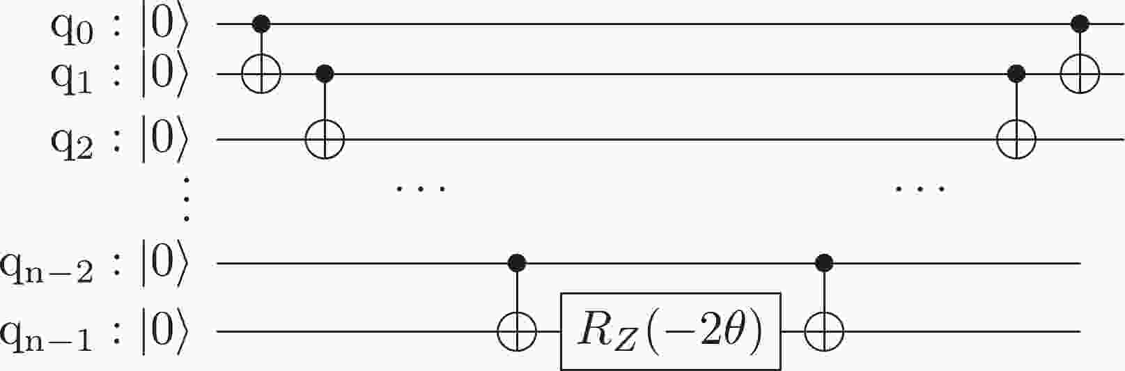
$ U(\theta) $ . The operator$\exp\left[ {\rm i} \theta Z_1 Z_2 \cdots Z_n\right]$ can be expressed as the following circuit: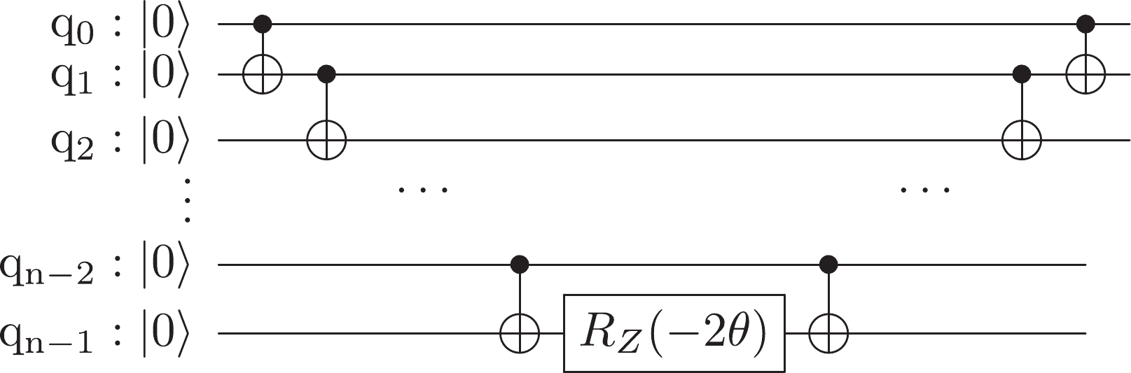
The operator
$\exp\left[ {\rm i} \theta Z_1 \cdots X_i \cdots Y_j \cdots Z_n\right]$ is expressed by inserting the rotation-y gates, that is,$ R_{Y}(\pi/2) $ and$ R_{Y}(-\pi/2) $ are placed at the first and last position of${q}_i$ , respectively, whereas$ R_{X}(\pi/2) $ and$ R_{X}(-\pi/2) $ are placed at the first and last position of${q}_j$ , respectively.Generally speaking, a unitary operator, which is a component of the UCC ansatz, is implemented on a quantum circuit with so-called Trotter errors. However, the unitary operators in this study do not cause Trotter errors because
$ a_i^{\dagger}a_j^{\dagger} $ and$ a_j a_i $ in the Hamiltonian always hold$ [a_i^{\dagger}a_j^{\dagger}, a_j a_i] = 0 $ . -
The SL ansatz can be generated by the Rotoselect algorithm [30] and summarized in Algorithm 1. This algorithm produces an ansatz for a given Hamiltonian so that the ansatz provides the minimum energy by changing the types of single-qubit gates. In this study, we prepare the rotation gates
$ R_{X} $ ,$ R_{Y} $ , and$ R_{Z} $ as single-qubit gates and select one of them at each position in the quantum circuit. We obtain the minimum energy with respect to the parameter θ at each rotation axis of the target gate that we are optimizing, while the other gates remain unchanged. Then, we choose the optimal rotation axis, which provides the minimum energy among all rotation axes. Following this, we iterate this calculation for all gates and obtain the ground-state energy. See Algorithm 1 for details. -
In this study, we compare the two ansatz, that is, the UCC ansatz and the SL ansatz, for the Lipkin model with
$ N = 3 $ and$ N = 4 $ .We calculate the ground-state energies with five different interaction strengths to examine the range of validity of the ansatz. All calculations are simulated in a classical computer. In each calculation, 1000 measurements are performed at each iteration of the parameter optimization. The following results are accumulated by repeating the calculation 50 times to estimate the amount of sampling noise.
Quantum circuits of the UCC ansatz with
$ N = 3 $ and$ N = 4 $ are shown in Fig. 1. Here,$ R_{X} $ ,$ R_{Y} $ , and$ R_{Z} $ represent the rotation operators with respect to the X-, Y-, and Z-axes, respectively, where$ \theta_n $ represent the parameters to be optimized in the calculation. The blue bars connecting two qubits are the CNOT gates, which are two-qubit operations. The circuit for$ N = 3 $ consists of 16 CNOT gates, 30 single-qubit gates, and 3 parameters; the circuit for$ N = 4 $ consists of 40 CNOT gates, 60 single-qubit gates, and 4 parameters.
Figure 1. (color online) Quantum circuits for the UCC ansatz with (a)
$ N = 3 $ and (b)$ N = 4 $ . Here,$ R_{X} $ ,$ R_{Y} $ , and$ R_{Z} $ represent the rotation operators with respect to the X-, Y-, and Z-axes, respectively, where$ \theta_n $ represent the parameters to be optimized in the calculation. The blue bars connecting two qubits are the CNOT gates, which are the two-qubit operations. The circuit for$ N = 3 $ consists of 16 CNOT gates, 30 single-qubit gates, and 3 parameters; the circuit for$ N = 4 $ consists of 40 CNOT gates, 60 single-qubit gates, and 4 parameters.An example of the obtained quantum circuits for the SL ansatz with
$ N = 3 $ is shown in Fig. 2. In general, the circuit for$ N = 3 $ consists of 6 CNOT gates and 9 single-qubit gates with parameters. However, some of the single-qubit gates can be selected as the identity operators I with no parameters. For example, there are 5 identity operators in the case shown in Fig. 2. For the case of$ N = 4 $ , the circuit consists of 12 CNOT gates and 16 single-qubit gates with parameters; however, once again, several can be selected as identity operators. We will discuss more on the quantum circuit for the SL ansatz later in the paper.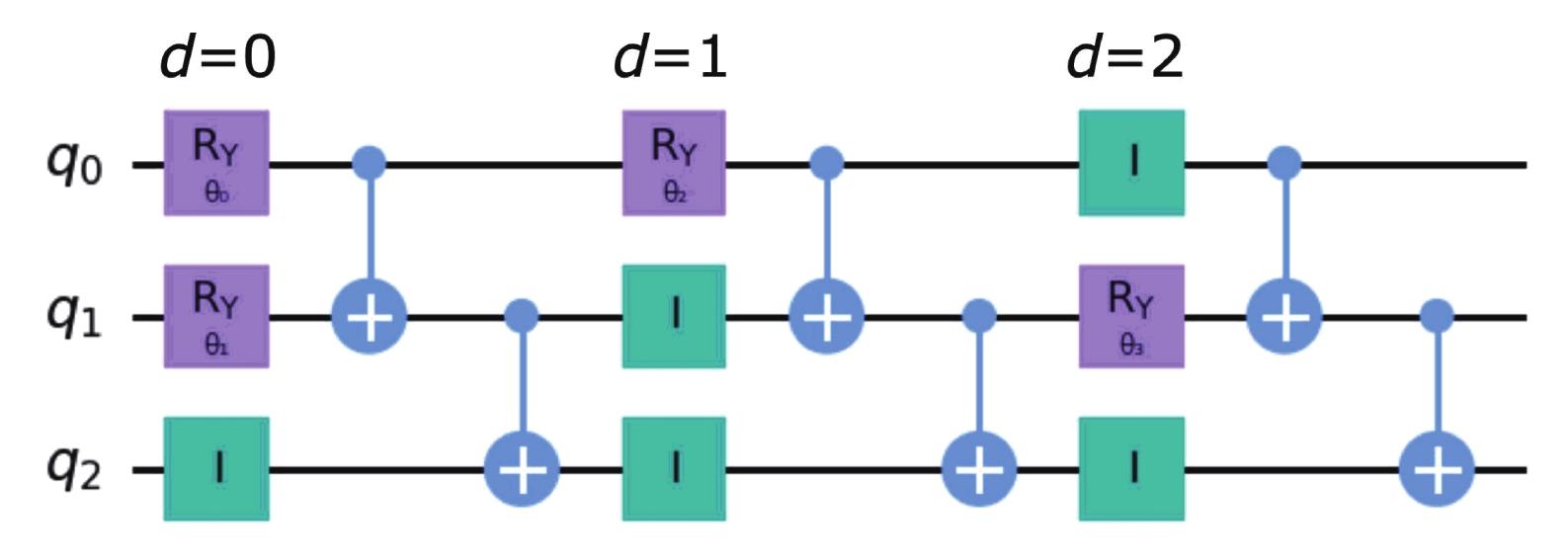
Figure 2. (color online) Example of obtained quantum circuit for SL ansatz with
$N=3$ . Here, I and$R_{Y}$ represent the identity and the rotation operator with respect to Y-axis, respectively. The blue bars which connect two qubits are the CNOT gates. Here, d is the depth of a quantum circuit, and$\theta_n$ represents the parameters to be optimized in the calculation. In this example, the circuit for$N=3$ consists of 6 CNOT gates, 4 single-qubit gates, and 4 parameters.First, the ground-state energies of the Lipkin model with
$ N = 3 $ and$ N = 4 $ are shown as a function of the interaction strength in Fig. 3. The calculated results with the UCC and SL ansatz are shown in the upper and lower panels, respectively. The distributions, medians, and quartiles of these results are shown by the so-called violin plots. For comparison, the corresponding exact ground-state energies are shown by solid lines. In general, the exact ground-state energies can be well reproduced by both the UCC and SL ansatz, and all the calculated energies are greater than the exact values. This is due to the variational principle.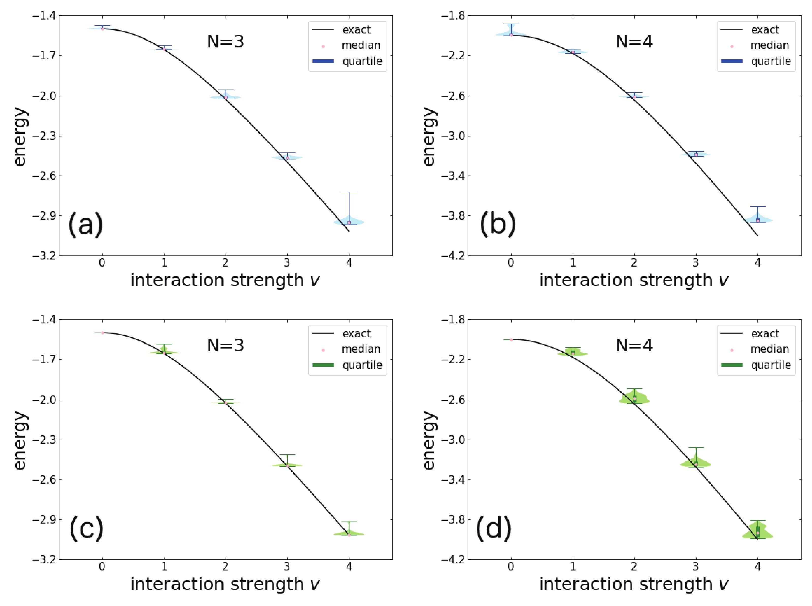
Figure 3. (color online) Ground-state energies of the Lipkin model with
$ N = 3 $ and$ N = 4 $ as a function of interaction strength. The calculated results with the UCC and SL ansatz are shown in the upper and lower panels, respectively. The distributions, medians, and quartiles of these results are shown by the so-called violin plots. For comparison, the corresponding exact ground-state energies are shown by the solid lines.For the UCC ansatz, the deviation between the calculated results and the exact ground-state energies gradually increases with increasing interaction strength. When
$ v = 4.0 $ , the mean relative errors$ (\bar E_{\rm{cal}} - E_{\rm{exact}})/ $ $ E_{\rm{exact}} $ reach 2.2% and 3.8% for the cases of$ N = 3 $ and$ N = 4 $ , respectively. Generally, a unitary operator in an ansatz is implemented on the quantum circuit with Trotter errors. However, the unitary operator in this study does not contribute to Trotter errors because of the commutability between$ a_i^{\dagger}a_j^{\dagger} $ and$ a_j a_i $ in the Lipkin model. Therefore, the difference between the exact energy and the energy with the UCC ansatz is not caused by Trotter errors.On the one hand, the calculated results by the SL ansatz are even better than those obtained by the UCC ansatz. It is found that when
$ v = 0 $ , all 50 calculations result in the exact ground-state energies. Moreover, the deviations between the calculated results and the exact values increase more gradually with increasing interaction strength. When$ v = 4.0 $ , the mean relative errors are 0.1% and 1.6% for the cases of$ N = 3 $ and$ N = 4 $ , respectively.On the other hand, for the
$ N = 4 $ case, the variances of the calculated results obtained by the SL ansatz are larger than those by the UCC ansatz. This is because the selected gates in each position, labelled by the depth d and the qubit index q, of the quantum circuit by the Rotoselect algorithm in each calculation differ. The options in each position include$ \{I, R_X, R_Y, R_Z\} $ .By taking
$ v = 0.0 $ , 2.0, and 4.0 as examples, we show the histograms of the ground-state energies calculated with the UCC and SL ansatz in Figs. 4 and 5, respectively. In these figures, the dotted pink lines show the corresponding exact ground-state energies.
Figure 4. (color online) Histograms of the ground-state energies calculated with the UCC ansatz and the 50 calculations. The dotted pink lines show the corresponding exact ground-state energies.
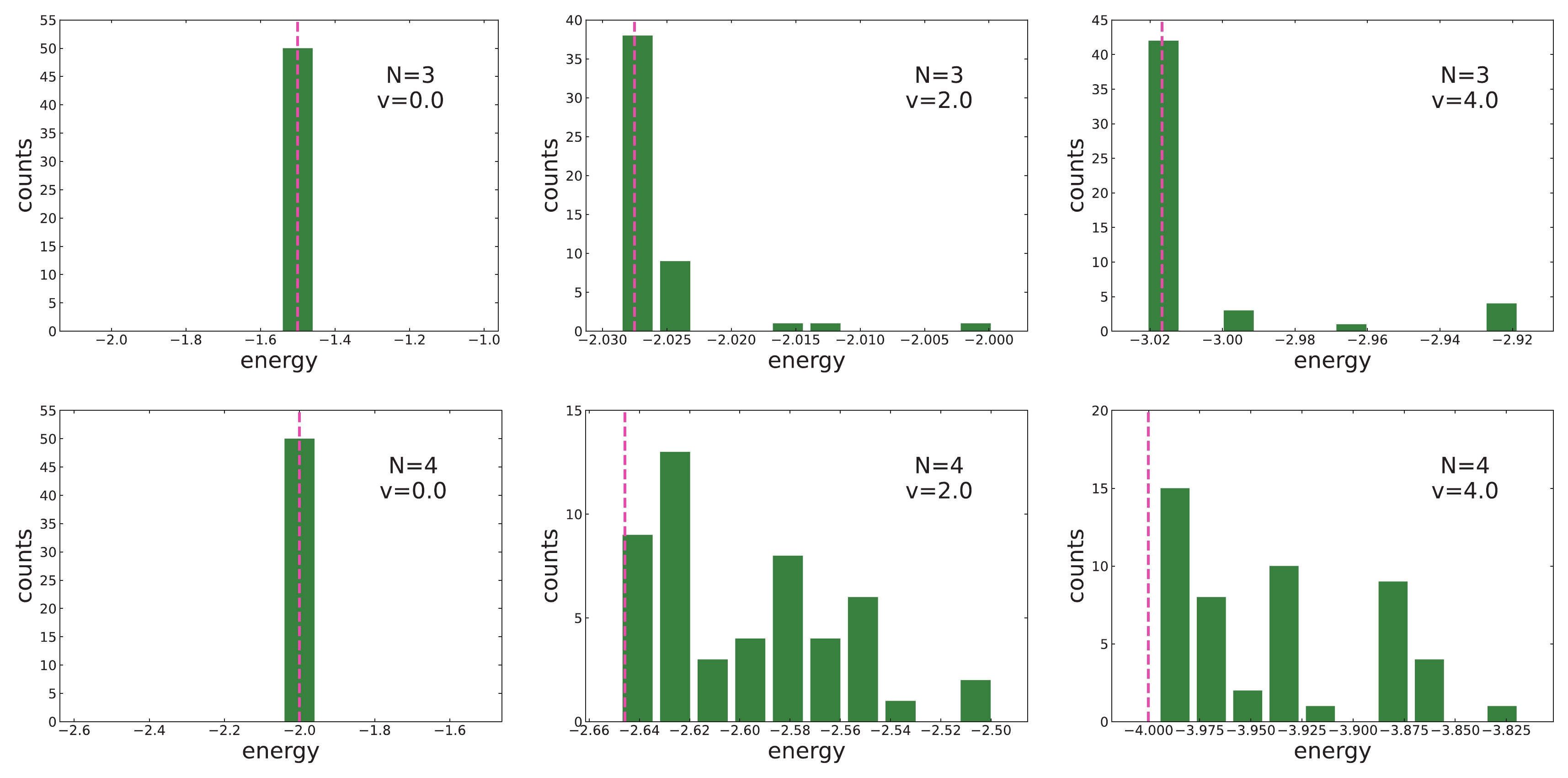
Figure 5. (color online) Same as Fig. 4, but for the results calculated with the SL ansatz.
For variational calculations, the obtained lowest energies represent the best results, that is, the closest results to the exact values. The difference between the best result with the UCC ansatz and the exact energy increases substantially as the interaction strength increases. In contrast, the difference between the best result with the SL ansatz and the exact energy only increases gradually with the increasing interaction strength. As a result, the obtained lowest energies with the SL ansatz are much closer to the exact values than those with the UCC ansatz. In addition, the variance with the UCC ansatz increases as the interaction strength increases. The variance with the SL ansatz for
$ N = 4 $ is larger than that for$ N = 3 $ , with more single-qubit gates selected by the Rotoselect algorithm.The obtained parameters of the UCC ansatz are shown in Fig. 6. The standard errors of the results with 50 calculations are too small to be seen in the figure. Each index of the rotation gate corresponds to each term in the UCC ansatz. For example, the parameter of the index 0 for
$ N = 3 $ corresponds to the operator$ e^{\theta_0 (a^{\dagger}_0 a^{\dagger}_1 - a_1 a_0)} $ . Note that the parameters at$ v = 0 $ for both cases of$ N = 3 $ and$ N = 4 $ are not 0 because the sampling noises affect parameter optimization. In general, the parameters increase as the interaction strength increases for both$ N = 3 $ and$ N = 4 $ . In addition, the difference between the parameters increases as the interaction strength increases for$ N = 3 $ . However, for$ N = 4 $ , the difference between the parameters is small, although the parameter of index 4 is not correctly optimized.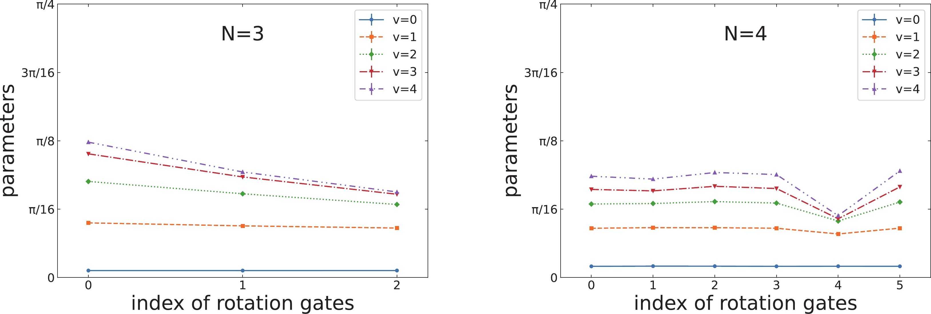
Figure 6. (color online) Parameters of the UCC ansatz with the 50 calculations. The horizontal axis corresponds to the index of each rotation gate.
An example of the obtained quantum circuits for the SL ansatz is shown in Fig. 2. In this example, the rotation gates
$ R_Y $ are selected in the positions$ (d, q) = $ (0, 0), (0, 1), (1, 0), (2, 1), the identity gates I are selected in$ (d, q) = $ (0, 2), (1, 1), (1, 2), (2, 0), (2, 2) , and no$ R_X $ nor$ R_Z $ gates are selected.For all 50 calculations, the statistics of the selected rotation axes at each qubit and each depth for the SL ansatz with the Rotoselect algorithm are shown in Fig. 7 for both cases of
$ N = 3 $ and$ N = 4 $ . The results of the selections vary in each calculation because of statistical errors. Because the selected gates are changed in each calculation, the variances in the obtained energies increase (see Fig. 5). It can be seen that$ R_{Y} $ is intensively selected at specific positions on the quantum circuit according to the 50 calculations. These results suggest that the rotation gate$ R_{Y} $ improves the expressibility of a parameterized quantum circuit.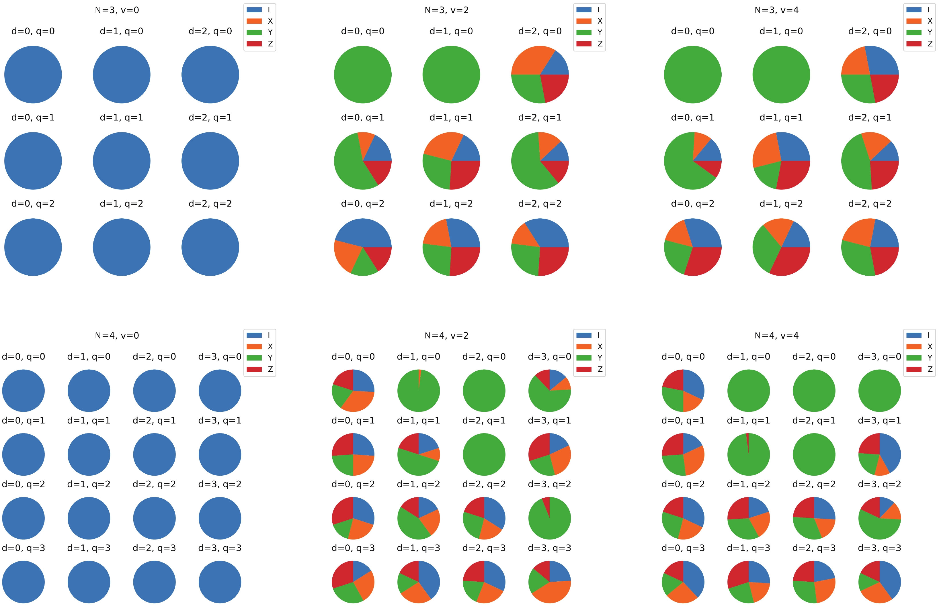
Figure 7. (color online) Selected rotation axes at each qubit and depth for the SL ansatz with
$ N = 3 $ and$ N = 4 $ . These data are generated with the 50 calculations. Here, N, v, d, and q are the number of particles, interaction strength, depth of a quantum circuit, and index of qubits, respectively.The optimized wave functions are shown in Figs. 8 and 9, where the vertical axes represent the probabilities, or precisely speaking, the probability amplitudes, of the obtained wave functions.
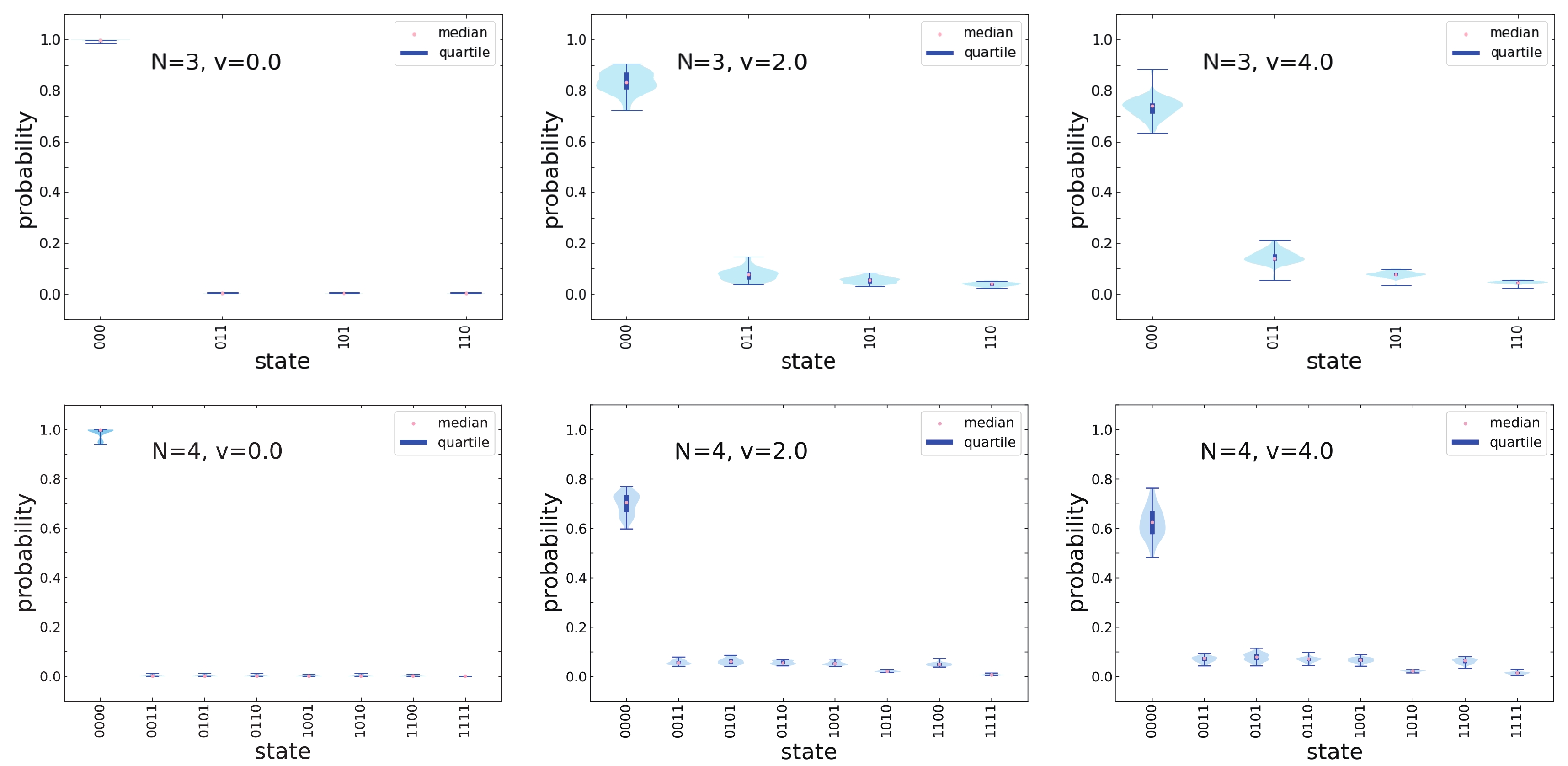
Figure 8. (color online) Probabilities of each state in the system ground-state wave function with the UCC ansatz. Their distributions, medians, and quartiles with the 50 calculations are shown by the violin plots. The upper panels represent the results with
$ N = 3 $ and the lower panels represent the results with$ N = 4 $ .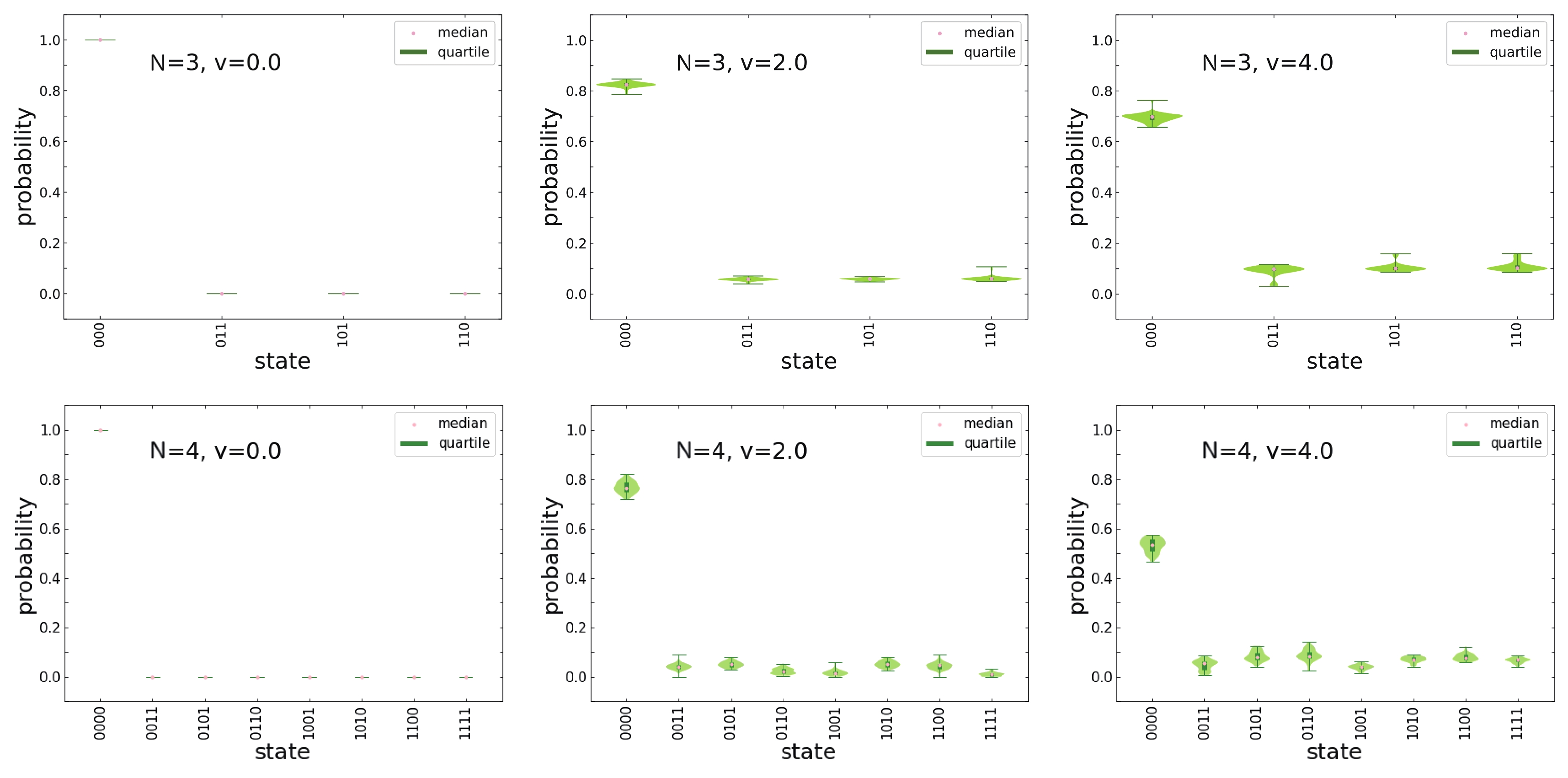
Figure 9. (color online) Same as Fig. 8, but for the results calculated with the SL ansatz.
Generally, system wave functions are represented by
$ \left| \Psi \right\rangle = \sum\limits_n c_n \left| n \right\rangle \;, $

(9) where
$ c_n $ is the coefficient of the state$ \left| n \right\rangle \equiv \left| {{n_1},{n_2}, \cdots ,{n_N}} \right\rangle $ . The corresponding probabilities$ P_n $ are$ P_n = |c_n|^2 \;, $

(10) which can be estimated by accumulating the statistics of the measurement outcomes of
$ \left| n \right\rangle $ in a quantum computer.The probabilities of each state in the system ground-state wave function are shown in Figs. 8 and 9 for the UCC and SL ansatz, respectively, where the violin plots show the corresponding distributions, medians, and quartiles with the 50 calculations. Owing to the symmetries of the Lipkin Hamiltonian, the states with the same number of single-particle excitations (that is, the same value of
$ n_1 + n_2 + \cdots + n_N $ ) should have the same probability. It can be seen from the figures that such a property is much better reproduced by the SL ansatz than the UCC ansatz, particularly for the strong interactions. This also indicates a problem in parameter optimization of the UCC ansatz. -
In this study, we applied two types of ansatz, the UCC and SL ansatz, to the Lipkin model and succeeded in obtaining the ground-state energy for all model interaction strengths. Generally, the errors between the results of the SL ansatz and the exact values are less than those by the UCC ansatz. For example, for the case of
$ N = 4 $ with the interaction strength$ v = 4 $ , the mean relative errors$ (\bar E_{\rm{cal}} - E_{\rm{exact}})/E_{\rm{exact}} $ in the SL and UCC ansatz are 1.6% and 3.8%, respectively. In addition, the quantum circuit of the SL ansatz requires fewer quantum gates, such as the CNOT gates and the rotation gates. In a future study, we will aim to apply the SL ansatz to the nuclear shell model, which is more realistic and a natural extension of the Lipkin model. -
We would like to thank the RIKEN iTHEMS program and the RIKEN Pioneering Project: Evolution of Matter in the Universe.
Quantum computing for the Lipkin model with unitary coupled cluster and structure learning ansatz
- Received Date: 2021-09-21
- Available Online: 2022-02-15
Abstract: We report a benchmark calculation for the Lipkin model in nuclear physics with a variational quantum eigensolver in quantum computing. Special attention is paid to the unitary coupled cluster (UCC) ansatz and structure learning (SL) ansatz for the trial wave function. Calculations with both the UCC and SL ansatz can reproduce the ground-state energy well; however, it is found that the calculation with the SL ansatz performs better than that with the UCC ansatz, and the SL ansatz has even fewer quantum gates than the UCC ansatz.


 DownLoad: