


 Abstract
 HTML
HTML Reference
 Related
 PDF
PDF


-
The study on exotic hadron states elucidates the property of QCD and also explores a new form of matter. However, the existence of exotic states remains an open question. Most of the exotic states can be classified in the conventional quark model, and the properties of the exotic states can be explained in the framework of the quark model with a few improvements. For example, the well-known exotic state [1-4],
$ X(3872) $ , can be explained as the traditional$ c\bar{c} $ state with a large component$ D\bar{D^*} + D^*\bar{D} $ in our unquenched quark model [5].In fact, several experimental collaborations have been searching for exotic states for the past two decades. In 2016, the D0 Collaboration observed a narrow structure, which is denoted as
$ X(5568) $ , in the$ B_{s}^{0}\pi^{\pm} $ invariant mass spectrum with a$ 5.1\sigma $ significance [6]. Owing to the$ B_{s}^{0}\pi^{\pm} $ decay mode,$ X(5568) $ was interpreted as the$ s\bar{d}u\bar{b}\; (s\bar{u}d\bar{b}) $ tetraquark state. However, it is difficult to determine the candidate for$ X(5568) $ in various approaches, if the requirements for ordinary hadrons can be described well in the approaches [7]. In our chiral quark model calculation, all the possible candidates for$ X(5568) $ are scattering states [8], while we predicted one shallow bound state [9, 10],$ B\bar{K} $ with$ 6.2 $ GeV, in the$ IJ^P = 00^+\; bs\bar{q}\bar{q} $ system. Indeed, other experimental collaborations did not find the existing evidence of$ X(5568) $ [11]. Recently, the LHCb Collaboration coincidentally reported their observation of the first two fully open-flavor tetraquark states named$ X_0(2900) $ and$ X_1(2900) $ in the$ cs\bar{q}\bar{q} $ system, whose statistical significance is more than$ 5\sigma $ [12]. If these two states are confirmed by other collaborations in the future, the$ X(2900) $ could be the first exotic state with four different flavors that cannot be quark-antiquark systems.$ \begin{array}{ll} M_{X_0(2900)} \hspace*{-3mm} &= 2866\pm 7 \;{\rm MeV}, \nonumber \\ \Gamma_{X_0(2900)} \hspace*{-3mm} &= 57\pm 3\; {\rm MeV}, \nonumber \\ M_{X_1(2900)} \hspace*{-3mm} &= 2904\pm 5\; {\rm MeV}, \nonumber \\ \Gamma_{X_1(2900)} \hspace*{-3mm} &= 110\pm 12 \;{\rm MeV}. \end{array} $

Owing to the report on
$ X(2900) $ , several possible candidates have emerged to elucidate$ X(2900) $ in different frameworks [13-30], and most of them can be divided into two categories: dimeson and diquark structures. Xue et al. obtained a$ 0^+ $ $ D^*\bar{K^*} $ resonance that can elucidate the$ X_0(2900) $ in the quark delocalization color screening model [13], and via the qBSE approach, He et al. also arrived at the same conclusion [14]. Karliner et al. approximately estimated the diquark structure of$ cs\bar{q}\bar{q} $ , and obtained a resonance that can be assigned as the candidate for$ X_0(2900) $ [22]. In addition, a resonance with$ J^{P} = 0^+ $ of$ bs\bar{q}\bar{q} $ system with a mass of$ 6.2 $ GeV was also proposed. In the framework of the QCD sum rule, Chen et al. assigned$ X_0(2900) $ as a$ 0^{+} $ $ D^*\bar{K^*} $ molecular state, while$ X_1(2900) $ was assigned as a$ 1^{-} $ $ cs\bar{q}\bar{q} $ diquark state [23]. However, using a similar method, Zhang regarded both$ X_0(2900) $ and$ X_1(2900) $ as diquark states [24]. In addition, before the report on$ X(2900) $ , Agaev et al. [25] obtained a resonance with$ 2878\pm 128 $ MeV in the$ 0^+ $ $ cs\bar{q}\bar{q} $ system. A few studies have also disfavored these findings. Liu et al. hypothesized that the two rescattering peaks may simulate the$ X(2900) $ without introducing genuine exotic states [28]. Burns et al. interpreted the$ X(2900) $ as a triangle cusp effect originating from$ D^*\bar{K^*} $ and$ D_1\bar{K} $ interactions [29]. Based on an extended relativized quark model, the study reported in [30] determined four resonances,$ 2765 $ ,$ 3055 $ ,$ 3152 $ , and$ 3396 $ MeV, and none of them could be the candidate for$ X_0(2900) $ in the$ 0^+ $ $ cs\bar{q}\bar{q} $ system.In fact, both molecular
$ D^*\bar{K^*} $ and diquark$ cs\bar{q}\bar{q} $ configurations have energies approximate to the mass of$ X(2900) $ . System dynamics should determine the preferred structure. Hence, the structure mixing calculation is required. Owing to the high energy of$ X(2900) $ , the combinations of the excited states of$ c\bar{q} $ and$ s\bar{q} $ are possible. More importantly, these states will couple with the decay channels,$ D\bar{K} $ ,$ D\bar{K^*} $ , and$ D^*\bar{K} $ . Do these states survive after the coupling? Owing to the finite space used in the calculation, a stability method has to be employed to identify the genuine resonance. In this study, a structure mixing calculation of meson-meson and diquark-antidiquark structures is performed in the framework of the chiral quark model via the Gaussian expansion method (GEM), and the excited states of subclusters are included. Therefore, four kinds of states with quantum numbers,$ IJ^P = 00^{\pm} $ and$ 01^{\pm} $ , are investigated. Owing to the lack of orbital-spin interactions in our calculation, we adopt the symbol$ ^{2S+1}L_J $ to denote P-wave excited states. Accordingly,$ 0^- $ and$ 1^- $ may be expressed as$ ^1P_1 $ ,$ ^3P_J $ , and$ ^5P_J $ . To determine the genuine resonance, the real-scaling method [31] is adopted.This paper is organized as follows. In Sec. II, the chiral quark model, real-scaling method, and the wave-function of
$ cs\bar{q}\bar{q} $ systems are presented. The numerical results are provided in Sec. III, and the last section summarizes the study. -
The constituent chiral quark model (ChQM) has been successful both in describing the hadron spectra and hadron-hadron interactions. Details on the model can be found in Refs. [32, 33]. The Hamiltonian of ChQM for the four-quark system is written as
$ \begin{aligned}[b] H = & \sum_{i = 1}^4 m_i+\frac{p_{12}^2}{2\mu_{12}}+\frac{p_{34}^2}{2\mu_{34}} +\frac{p_{1234}^2}{2\mu_{1234}} \\ & + \sum_{i<j = 1}^4 \left( V_{ij}^{G}+V_{ij}^{C}+\sum_{\chi = \pi,K,\eta} V_{ij}^{\chi}+V_{ij}^{\sigma} \right), \end{aligned} $

(1) where
$ m_i $ is the constituent mass of the i-th quark (antiquark), and$ \mu $ is the reduced mass of two interacting quarks or quark-clusters.$ \begin{aligned}[b] \mu_{ij} &= \frac{m_{{i}} m_{{j}}}{m_{{i}} + m_{{j}}}, \; \; \;\; \mu_{1234} = \frac{(m_1+m_2)(m_3+m_4)}{m_1+m_2+m_3+m_4}, \\ p_{ij} &= \frac{m_jp_i-m_ip_j}{m_i+m_j}, \\ p_{1234} &= \frac{(m_3+m_4)p_{12}-(m_1+m_2)p_{34}}{m_1+m_2+m_3+m_4}. \end{aligned} $

(2) The quadratic form of color confinement is used here:
$ V_{ij}^{C} = ( -a_{c} r_{ij}^{2}-\Delta) \boldsymbol{\lambda}_i^c \cdot \boldsymbol{\lambda}_j^c . $

(3) The effective smeared one-gluon exchange interaction takes the form
$ \begin{aligned}[b] V_{ij}^{G} &= \frac{\alpha_s}{4} \boldsymbol{\lambda}_i^c \cdot \boldsymbol{\lambda}_{j}^c \left[\frac{1}{r_{ij}}-\frac{2\pi}{3m_im_j}\boldsymbol{\sigma}_i\cdot \boldsymbol{\sigma}_j \delta(\boldsymbol{r}_{ij})\right], \\ \delta{(\boldsymbol{r}_{ij})} &= \frac{{\rm e}^{-r_{ij}/r_0(\mu_{ij})}}{4\pi r_{ij}r_0^2(\mu_{ij})},\; \; \;\; r_{0}(\mu_{ij}) = \frac{r_0}{\mu_{ij}}. \end{aligned} $

(4) The last piece of the potential is the Goldstone boson exchange, which originates from the effects of the chiral symmetry spontaneous breaking of QCD in the low-energy region,
$ \begin{aligned}[b] V_{ij}^{\pi} = & \frac{g_{ch}^2}{4\pi}\frac{m_{\pi}^2}{12m_im_j} \frac{\Lambda_{\pi}^2}{\Lambda_{\pi}^2-m_{\pi}^2}m_\pi v_{ij}^{\pi} \sum_{a = 1}^3 \lambda_i^a \lambda_j^a, \\ V_{ij}^{K} = & \frac{g_{ch}^2}{4\pi}\frac{m_{K}^2}{12m_im_j} \frac{\Lambda_K^2}{\Lambda_K^2-m_{K}^2}m_K v_{ij}^{K} \sum_{a = 4}^7 \lambda_i^a \lambda_j^a, \\ V_{ij}^{\eta} = & \frac{g_{ch}^2}{4\pi}\frac{m_{\eta}^2}{12m_im_j} \frac{\Lambda_{\eta}^2}{\Lambda_{\eta}^2-m_{\eta}^2}m_{\eta} v_{ij}^{\eta} \\ &\times \left[\lambda_i^8 \lambda_j^8 \cos\theta_P - \lambda_i^0 \lambda_j^0 \sin \theta_P \right], \\ V_{ij}^{\sigma} =& -\frac{g_{ch}^2}{4\pi} \frac{\Lambda_{\sigma}^2}{\Lambda_{\sigma}^2-m_{\sigma}^2}m_\sigma \left[ Y(m_\sigma r_{ij})-\frac{\Lambda_{\sigma}}{m_\sigma}Y(\Lambda_{\sigma} r_{ij})\right], \\ v_{ij}^{\chi} =& \left[ Y(m_\chi r_{ij})- \frac{\Lambda_{\chi}^3}{m_{\chi}^3}Y(\Lambda_{\chi} r_{ij}) \right] \boldsymbol{\sigma}_i \cdot\boldsymbol{\sigma}_j, \\ Y(x) =&\, {\rm e}^{-x}/x . \end{aligned} $

(5) In the above expressions,
$ \boldsymbol{\sigma} $ indicates the$ SU(2) $ Pauli matrices;$ \boldsymbol{\lambda} $ and$ \boldsymbol{\lambda}^{c} $ are the$ SU(3) $ flavor and color Gell-Mann matrices, respectively; and$ \alpha_{s} $ is an effective scale-dependent running coupling,$ \alpha_s(\mu_{ij}) = \frac{\alpha_0}{\ln\left[(\mu_{ij}^2+\mu_0^2)/\Lambda_0^2\right]}. $

(6) The model parameters are determined by the requirement that the model can accommodate all the ordinary mesons, from light to heavy, considering only a quark-antiquark component. Details on the meson spectrum fitting process can be found in the work by Vijande et al. [32]. Here, we provide a brief introduction of the process. First, the mass parameters,
$ m_{s},s = \sigma,\eta,\kappa,\pi $ take their experimental values, while the cut-off parameters,$ \Lambda_{s},s = $ $ \sigma,\eta,\kappa,\pi $ , are fixed at typically used values [32]. Second, the chiral coupling constant$ g_{ch} $ can be obtained from the experimental value of the$ \pi NN $ coupling constant$ \frac{g_{ch}^2}{4\pi} = \frac{9}{25} \frac{g^2_{\pi NN}}{4\pi}\frac{m_{ud}^2}{m_N^2}. $

Finally, our confinement potential takes the ordinary quadratic form, which differs from the expression used in Ref. [32], where the effect of sea quark excitation is considered. Here, we leave the effect of sea quark excitation to the unquenched quark model. All of the parameters are presented in Table 1, and the masses of mesons obtained are presented in Table 2.
Quark masses $m_u = m_d$ /MeV

313 $m_{s}$ /MeV

536 $m_{c}$ /MeV

1728 $m_{b}$ /MeV

5112 Goldstone bosons $\Lambda_{\pi} = \Lambda_{\sigma}$ /fm

$^{-1}$ 

4.2 $\Lambda_{\eta} = \Lambda_{K}$ /fm

$^{-1}$ 

5.2 $g_{ch}^2/(4\pi)$ 

0.54 $\theta_p/(^\circ)$ 

−15 Confinement $a_{c}$ /MeV

101 $\Delta$ /MeV

−78.3 $\mu_{c}$ /MeV

0.7 OGE $\alpha_{0}$ 

3.67 $\Lambda_{0}$ /fm

$^{-1}$ 

0.033 $\mu_0$ /MeV

36.976 $\hat{r}_0$ /MeV

28.17 Table 1. Quark Model Parameters (
$m_{\pi} = 0.7$ fm−1,$m_{\sigma} = 3.42$ fm−1,$m_{\eta} = 2.77$ fm−1, and$m_{K} = 2.51$ fm−1).$D$ 

$D^*$ 

$D_J$ 

$D_1$ 

QM 1862.6 1980.5 2454.7 2448.1 exp 1867.7 2008.9 2420.0 2420.0 $K$ 

$K^*$ 

$K_J$ 

$K_1$ 

QM 493.9 913.6 1423.0 1400.0 exp 495.0 892.0 1430.0 1427.0 Table 2. Meson spectrum (unit: MeV).
-
The
$ cs\bar{q}\bar{q} $ system has two structures, meson-meson and diquark-antidiquark, and the wave function of each structure comprises four parts: orbital, spin, flavor, and color wave functions. In addition, the wave function of each part is constructed by coupling two sub-clusters wave functions. Therefore, the wave function for each channel will be the tensor product of the orbital ($ |R_{i}\rangle $ ), spin ($ |S_{j}\rangle $ ), color ($ |C_{k}\rangle $ ) and flavor ($ |F_{l}\rangle $ ) components,$ |ijkl\rangle = {\cal A} |R_{i}\rangle\otimes|S_{j}\rangle\otimes|C_{k}\rangle\otimes|F_{l}\rangle ,$

(7) $ {\cal A} $ is the antisymmetrization operator. -
The orbital wave function comprises two sub-clusters orbital wave functions and the relative motion wave function between two sub-clusters,
$ \begin{array}{l} \Phi(r) = \sum C_{l_1,l_2,l_3}^{L} \Psi_{l_1}({\boldsymbol r}_{12})\Psi_{l_2}({\boldsymbol r}_{34}) \Psi_{l_3}({\boldsymbol r}_{1234}). \\ \end{array} $

(8) The negative parity requires the P-wave angular momentum, and only one orbital angular momentum is set to 1. Accordingly, the following combinations are obtained:
$ l_1 = 1, $ $ l_2 = 0,\;l_3 = 0 $ as "$ |R_{1}\rangle $ ,"$ l_1 = 0,\;l_2 = 1,\;l_3 = 0 $ as "$ |R_{2}\rangle $ ," and$ l_1 = 0,\;l_2 = 0,\;l_3 = 1 $ as "$ |R_{3}\rangle $ ." However, for the positive parity state, we set all orbital angular momentum to 0,$ l_1 = 0,\;l_2 = 0,\;l_3 = 0 $ as "$ |R_{0}\rangle $ ."In the GEM, the radial part of the spatial wave function is expanded by Gaussians:
$ R(\boldsymbol{r}) = \sum_{n = 1}^{n_{\rm max}} c_{n}\psi^G_{nlm}(\boldsymbol{r}), $

(9) $ \psi^G_{nlm}(\boldsymbol{r}) = N_{nl}r^{l} {\rm e}^{-\nu_{n}r^2}Y_{lm}(\hat{\boldsymbol{r}}), $

(10) where
$ N_{nl} $ , which is the normalization constant, is expressed as$ N_{nl} = \left[\frac{2^{l+2}(2\nu_{n})^{l+\frac{3}{2}}}{\sqrt{\pi}(2l+1)} \right]^\frac{1}{2}. $

(11) $ c_n $ are the variational parameters, which are determined dynamically. The Gaussian size parameters are selected according to the following geometric progression$ \nu_{n} = \frac{1}{r^2_n}, \quad r_n = r_1a^{n-1}, \quad a = \left(\frac{r_{n_{\rm max}}}{r_1}\right)^{\frac{1}{n_{\rm max}-1}}. $

(12) The advantage of the geometric progression is that it enables the optimization of the ranges using just a small number of Gaussians. The GEM has been successfully used in the calculation of few-body systems [34].
-
Because there is no difference between the spin of quark and antiquark, the wave functions of the meson-meson structure has the same form as that of the diquark-antidiquark structure.
$ \begin{aligned}[b] |S_{1}\rangle = & \chi_{0}^{\sigma1} = \chi_{00}^{\sigma}\chi_{00}^{\sigma}, \\ |S_{2}\rangle =& \chi_{0}^{\sigma2} = \sqrt{\frac{1}{3}}(\chi_{11}^{\sigma}\chi_{1-1}^{\sigma} -\chi_{10}^{\sigma}\chi_{10}^{\sigma}+\chi_{1-1}^{\sigma}\chi_{11}^{\sigma}), \\ |S_{3}\rangle =& \chi_{1}^{\sigma1} = \chi_{00}^{\sigma}\chi_{11}^{\sigma}, \\ |S_{4}\rangle =& \chi_{1}^{\sigma2} = \chi_{11}^{\sigma}\chi_{00}^{\sigma}, \\ |S_{5}\rangle =& \chi_{1}^{\sigma3} = \frac{1}{\sqrt{2}}(\chi_{11}^{\sigma}\chi_{10}^{\sigma}-\chi_{10}^{\sigma}\chi_{11}^{\sigma}), \\ |S_{6}\rangle = & \chi_{2}^{\sigma1} = \chi_{11}^{\sigma}\chi_{11}^{\sigma}. \end{aligned} $

(13) Where the subscript of "
$ \chi_{S}^{\sigma i} $ " denotes the total spin of the tretraquark, and the superscript is the index of the spin function with a fixed S. -
The total flavor wave functions can be written as,
$ \begin{aligned}[b] |F_{1}\rangle = & \frac{1}{\sqrt{2}}\left( c\bar{u}s\bar{d}- c\bar{d}s\bar{u} \right), \\ |F_{2}\rangle =& \frac{1}{\sqrt{2}}\left( cs\bar{u}\bar{d}- cs\bar{d}\bar{u} \right). \end{aligned} $

(14) Here,
$ |F_{1}\rangle $ ($ |F_{2}\rangle $ ) denotes the flavor wave function for the molecular (diquark-antidiquark) structure. -
The colorless tetraquark system has four color structures, including
$ 1\otimes1 $ ,$ 8\otimes8 $ ,$ 3\otimes \bar{3} $ , and$ 6\otimes \bar{6} $ ,$ \begin{aligned}[b] |C_{1}\rangle = & \chi_{1\otimes1}^{m1} = \frac{1}{\sqrt{9}}(\bar{r}r\bar{r}r+\bar{r}r\bar{g}g+\bar{r}r\bar{b}b +\bar{g}g\bar{r}r+\bar{g}g\bar{g}g \\ & + \bar{g}g\bar{b}b+\bar{b}b\bar{r}r+\bar{b}b\bar{g}g+\bar{b}b\bar{b}b), \end{aligned} $

$ \begin{aligned}[b]|C_{2}\rangle =\; & \chi_{8\otimes8}^{m2} = \frac{\sqrt{2}}{12}(3\bar{b}r\bar{r}b+3\bar{g}r\bar{r}g+3\bar{b}g\bar{g}b +3\bar{g}b\bar{b}g \\& + 3\bar{r}g\bar{g}r+ 3\bar{r}b\bar{b}r+2\bar{r}r\bar{r}r+2\bar{g}g\bar{g}g+2\bar{b}b\bar{b}b-\bar{r}r\bar{g}g \\ & - \bar{g}g\bar{r}r-\bar{b}b\bar{g}g-\bar{b}b\bar{r}r-\bar{g}g\bar{b}b-\bar{r}r\bar{b}b). \\ |C_{3}\rangle =\; & \chi^{d1}_{\bar{3}\otimes 3} = \frac{\sqrt{3}}{6}(rg\bar{r}\bar{g}-rg\bar{g}\bar{r}+gr\bar{g}\bar{r} -gr\bar{r}\bar{g}+rb\bar{r}\bar{b}, \\ & - rb\bar{b}\bar{r}+br\bar{b}\bar{r}-br\bar{r}\bar{b}+gb\bar{g}\bar{b}-gb\bar{b}\bar{g}+bg\bar{b}\bar{g}-bg\bar{g}\bar{b}), \\ |C_{4}\rangle =\; & \chi^{d2}_{6\otimes \bar{6}} = \frac{\sqrt{6}}{12}(2rr\bar{r}\bar{r}+2gg\bar{g}\bar{g}+2bb\bar{b}\bar{b} +rg\bar{r}\bar{g} \\& + rg\bar{g}\bar{r}+gr\bar{g}\bar{r}+gr\bar{r}\bar{g}+rb\bar{r}\bar{b}+rb\bar{b}\bar{r}+br\bar{b}\bar{r} \\& + br\bar{r}\bar{b}+gb\bar{g}\bar{b}+gb\bar{b}\bar{g}+bg\bar{b}\bar{g}+bg\bar{g}\bar{b}). \end{aligned} $

(15) To write down the wave functions easily for each structure, the different orders of particles are adopted. However, when coupling the different structure, the same order of particles should be used.
-
In this study, we investigated all possible candidates for
$ X(2900) $ in the$ cs\bar{q}\bar{q} $ system. The antisymmetrization operators are different for different structures. For the$ cs\bar{q}\bar{q} $ system, the antisymmetrization operator becomes$ {\cal A} = 1-(34) $

(16) for diquark-antidiquark, and
$ {\cal A} = 1-(24) $

(17) for the meson-meson structure. After applying the antisymmetrization operator, some wave function will vanish, which means that the states are forbidden. All of the allowed channels are presented in Table 3. The subscript "8" denotes the color octet subcluster, the superscript of the diquark/antidiquark is the spin of the subcluster, and the subscript is the color representation of subcluster,
$ 3 $ ,$ \bar{3} $ ,$ 6 $ and$ \bar{6} $ , which denote the color triplet, anti-triplet, sextet, and anti-sextet, respectively.$cs\bar{q}\bar{q}$ 

$ |ijkl\rangle $ 

$^3P_J $ 

$ |ijkl\rangle $ 

$^1P_1 $ 

$ |ijkl\rangle $ 

$^5P_J$ 

$ |1311\rangle $ 

$ D_1 \bar{K^*} $ 

$ |1111\rangle $ 

$ D_1 \bar{K} $ 

$ |1611\rangle $ 

$ D_J \bar{K^*} $ 

$ |1312\rangle $ 

$[D_1]_8[\bar{K^*}]_8 $ 

$ |1112\rangle $ 

$[D_1]_8[\bar{K}]_8 $ 

$ |1612\rangle $ 

$[D_J]_8[\bar{K^*}]_8 $ 

$ |1411\rangle $ 

$ D_J \bar{K} $ 

$ |1211\rangle $ 

$ D_J \bar{K^*} $ 

$ |2611\rangle $ 

$ D^* \bar{K_J} $ 

$ |1412\rangle $ 

$[D_J]_8[\bar{K}]_8 $ 

$ |1212\rangle $ 

$[D_J]_8[\bar{K^*}]_8 $ 

$ |2612\rangle $ 

$[D^*]_8[\bar{K_J}]_8 $ 

$ |1511\rangle $ 

$ D_J \bar{K^*}$ 

$ |2111\rangle $ 

$ D \bar{K_1}$ 

$ |3611\rangle $ 

$ (D^* \bar{K^*})_P $ 

$ |1512\rangle $ 

$[D_J]_8[\bar{K^*}]_8$ 

$ |2112\rangle $ 

$[D]_8[\bar{K_1}]_8$ 

$ |3612\rangle $ 

$([D^*]_8[\bar{K^*}]_8)_P $ 

$ |2311\rangle $ 

$ D \bar{K_J}$ 

$ |2211\rangle $ 

$ D^* \bar{K_J}$ 

$ |1624\rangle $ 

$[cs]_6^{1,P} [\bar{q}\bar{q}]_{\bar{6}}^1$ 

$ |2312\rangle $ 

$[D]_8[\bar{K_J}]_8 $ 

$ |2212\rangle $ 

$[D^*]_8[\bar{K_J}]_8$ 

$ |2623\rangle $ 

$[cs]_3^1 [\bar{q}\bar{q}]_{\bar{3}}^{1,P}$ 

$ |2411\rangle $ 

$ D^* \bar{K_1} $ 

$ |3111\rangle $ 

$ (D \bar{K})_P$ 

$ |3624\rangle $ 

$([cs]_6^1 [\bar{q}\bar{q}]_{\bar{6}}^1)_P$ 

$ |2412\rangle $ 

$[D^*]_8[\bar{K_1}]_8 $ 

$ |3112\rangle $ 

$([D]_8[\bar{K}]_8)_P$ 

$ |ijkl\rangle $ 

$1^+ $ 

$ |2511\rangle $ 

$ D^* \bar{K_J} $ 

$ |3211\rangle $ 

$ (D^* \bar{K}^*)_P$ 

$ |0311\rangle $ 

$D \bar{K^*}$ 

$ |2512\rangle $ 

$[D^*]_8[\bar{K_J}]_8$ 

$ |3212\rangle $ 

$([D^*]_8[\bar{K}^*]_8)_P$ 

$ |0312\rangle $ 

$[D]_8[\bar{K^*}]_8$ 

$ |3311\rangle $ 

$(D \bar{K}^*)_P$ 

$ |1123\rangle $ 

$[cs]_3^{0,P} [\bar{q}\bar{q}]_{\bar{3}}^0$ 

$ |0411\rangle $ 

$D^* \bar{K}$ 

$ |3312\rangle $ 

$([D]_8[\bar{K}^*]_8)_P$ 

$ |1224\rangle $ 

$[cs]_6^{1,P} [\bar{q}\bar{q}]_{\bar{6}}^1$ 

$ |0412\rangle $ 

$[D^*]_8[\bar{K}]_8$ 

$ |3411\rangle $ 

$(D^* \bar{K})_P$ 

$ |2124\rangle $ 

$[cs]_6^0 [\bar{q}\bar{q}]_{\bar{6}}^{1,P}$ 

$ |0511\rangle $ 

$D^* \bar{K^*}$ 

$ |3412\rangle $ 

$([D^*]_8[\bar{K}]_8)_P$ 

$ |2223\rangle $ 

$[cs]_3^1 [\bar{q}\bar{q}]_{\bar{3}}^{1,P}$ 

$ |0512\rangle $ 

$[D^*]_8[\bar{K^*}]_8$ 

$ |3511\rangle $ 

$(D^* \bar{K}^*)_P$ 

$ |3123\rangle $ 

$([cs]_3^0 [\bar{q}\bar{q}]_{\bar{3}}^0)_P$ 

$ |0324\rangle $ 

$[cs]_6^0 [\bar{q}\bar{q}]_{\bar{6}}^1$ 

$ |3512\rangle $ 

$([D^*]_8[\bar{K}^*]_8)_P$ 

$ |1324\rangle $ 

$[cs]_6^{1,P} [\bar{q}\bar{q}]_{\bar{6}}^1$ 

$ |0423\rangle $ 

$[cs]_3^1 [\bar{q}\bar{q}]_{\bar{3}}^0$ 

$ |1324\rangle $ 

$[cs]_6^{0,P} [\bar{q}\bar{q}]_{\bar{6}}^1$ 

$ |ijkl\rangle $ 

$0^+ $ 

$ |0524\rangle $ 

$[cs]_6^1 [\bar{q}\bar{q}]_{\bar{6}}^1$ 

$ |1423\rangle $ 

$[cs]_3^{1,P} [\bar{q}\bar{q}]_{\bar{3}}^0$ 

$ |0111\rangle $ 

$D \bar{K}$ 

$ |1524\rangle $ 

$[cs]_6^{1,P} [\bar{q}\bar{q}]_{\bar{6}}^1$ 

$ |0112\rangle $ 

$[D]_8[\bar{K}]_8$ 

$ |2323\rangle $ 

$[cs]_3^0 [\bar{q}\bar{q}]_{\bar{3}}^{1,P}$ 

$ |0211\rangle $ 

$D^* \bar{K^*}$ 

$ |2424\rangle $ 

$[cs]_6^1 [\bar{q}\bar{q}]_{\bar{6}}^{0,P}$ 

$ |0212\rangle $ 

$[D^*]_8[\bar{K^*}]_8$ 

$ |2523\rangle $ 

$[cs]_3^1 [\bar{q}\bar{q}]_{\bar{3}}^{1,P}$ 

$ |0123\rangle $ 

$[cs]_3^0 [\bar{q}\bar{q}]_{\bar{3}}^0$ 

$ |3324\rangle $ 

$([cs]_6^0 [\bar{q}\bar{q}]_{\bar{6}}^1)_P$ 

$ |0224\rangle $ 

$[cs]_6^1 [\bar{q}\bar{q}]_{\bar{6}}^1$ 

$ |3423\rangle $ 

$([cs]_3^1 [\bar{q}\bar{q}]_{\bar{3}}^0)_P$ 

$ |3524\rangle $ 

$([cs]_6^1 [\bar{q}\bar{q}]_{\bar{6}}^1)_P$ 

Table 3. All of the allowed channels. We adopt
$|ijkl\rangle$ to donate different states. "$i,j,k,l$ " are indices that denote the orbital, spin, flavor, and color wave functions, respectively. -
In this section, we present our numerical results. In the calculation of the
$ cs\bar{q}\bar{q} $ system, two structures, the meson-meson and diquark-antidiquark structures, and their coupling are considered. Because the mass of$ X(2900) $ is larger than the threshold of the$ cs\bar{q}\bar{q} $ system, the possible candidates must be resonance states rather than bound states. To verify whether the states survive the coupling to the open channels,$ D\bar{K} $ ,$ D\bar{K^*} $ , and$ D^*\bar{K} $ , the real-scaling method (RSM) is employed to test stability of these candidates. -
In the
$ J^P = 0^+\; cs\bar{q}\bar{q} $ system, there are four channels in the meson-meson structure and two channels in the diquark-antidiquark structure (see Table 3). The lowest eigen-energy of each channel is provided in the second column of Table 4. The eigen-energies of the entire channel coupling are presented in the rows that are marked "c.c," and the percentages in the table represent the percent of each channel in the eigen-states with corresponding energies (in the last row of the table). The two lowest eigen-energies and the eigen-energies of approximately$ 2900 $ MeV are given. In the channel coupling calculation, we obtain four energy levels,$ E_1(2836) $ ,$ E_2(2896) $ ,$ E_3(2906) $ and$ E_4(2936) $ , which could be the candidates for$ X_0(2900) $ . However, the eigen-state with$ E_2(2896) $ has ~89% of$ D^*\bar{K^*} $ , and the energy is higher than its threshold,$ 2894 $ MeV, and the single-channel calculation of$ D^*\bar{K^*} $ indicates that the state is unbound, such that it should be in a$ D^*\bar{K^*} $ scattering state rather than a resonance; hence,$ E_9(2906) $ does satisfy this. However, both$ E_1(2837) $ and$ E_4(2936) $ have more than 30% of the diquark structure, which indicates that the two states may be in resonance states. The stability of these states have to be verified when assigning these resonances to be the candidate for$ X_0(2900) $ .$0^{+}\; cs\bar{q}\bar{q}$ 

s.c. 1st 2nd − 7th 8th 9th 10th $ D \bar{K} $ 

$2357.0$ 

90.1% 99.4% − 61.9% 6.1% 24.0% 26.2% $[D]_8[\bar{K}]_8 $ 

$3098.2$ 

0.3% 0.0% − 1.5% 0.4% 0.9% 4.2% $ D^* \bar{K^*} $ 

$2895.8$ 

0.5% 0.0% − 0.3% 88.8% 58.8% 28.9% $[D^*]_8[\bar{K^*}]_8 $ 

$2863.7$ 

1.5% 0.1% − 2.6% 0.1% 1.5% 0.4% $ [cs]_3^0 [\bar{q}\bar{q}]_{\bar{3}}^0$ 

$2656.5$ 

6.9% 0.1% − 7.3% 0.3% 10.1% 0.9% $ [cs]_6^1 [\bar{q}\bar{q}]_{\bar{6}}^1$ 

$2965.7$ 

0.7% 0.4% − 26.3% 4.4% 4.9% 29.8% c.c. $2340.1$ 

$2358.9$ 

− $2836.3$ 

$2896.7$ 

$2906.9$ 

$2935.8$ 

$1^{+}\; cs\bar{q}\bar{q}$ 

s.c. 1st − 10th 11th 12th 13th 14th $ D \bar{K^*} $ 

$2777.6$ 

0.3% − 25.4% 0.5% 0.4% 0.2% 9.3% $[D]_8[\bar{K^*}]_8 $ 

$3111.8$ 

0.4% − 3.4% 1.1% 1.2% 1.7% 0.4% $ D^*\bar{K} $ 

$2475.3$ 

87.4% − 34.2% 30.1% 55.2% 63.7% 54.8% $[D^*]_8[\bar{K}]_8 $ 

$3110.7$ 

0.4% − 1.6% 0.6% 1.8% 1.2% 0.9% $ D^* \bar{K^*} $ 

$2895.9$ 

0.3% − 0.6% 52.5% 11.1% 3.7% 0.9% $[D^*]_8[\bar{K^*}]_8 $ 

$3005.0$ 

1.1% − 0.9% 1.5% 2.8% 3.4% 4.6% $ [cs]_6^0 [\bar{q}\bar{q}]_{\bar{6}}^1 $ 

$3112.3$ 

0.1% − 0.4% 1.2% 7.3% 4.8% 19.7% $ [cs]_3^1 [\bar{q}\bar{q}]_{\bar{3}}^0 $ 

$2690.6$ 

9.8% − 0.5% 1.2% 0.8% 4.5% 5.5% $ [cs]_6^1 [\bar{q}\bar{q}]_{\bar{6}}^1 $ 

$3040.4$ 

0.1% − 16.1% 11.4% 19.4% 17.0% 3.9% c.c. $2464.3$ 

− $2857.1$ 

$2896.3$ 

$2904.2$ 

$2920.3$ 

$2941.7$ 

Table 4. Results for
$IJ^P = 0^+,1^+$ states ("c.c." means channel coupling).Due to three combinations of spin in the
$ J^P = 1^+\; cs\bar{q}\bar{q} $ system, more channels are presented in Table 3. Consequently, five energy levels near$ X(2900) $ , which include$ E_5(2857) $ ,$ E_6(2896) $ ,$ E_7(2904) $ ,$ E_8(2920) $ , and$ E_9(2941) $ emerge in the channel coupling calculation. Similar to the$ J^P = 0^+ $ case, the$ E_6(2896) $ and$ E_7(2904) $ are dominated by the meson-meson scattering states. However, both$ E_8(2920) $ and$ E_9(2941) $ have almost 28% of the diquark structure, which is beneficial to the existence of resonance.For the P-wave excited
$ cs\bar{q}\bar{q} $ system, the states are denoted as$ ^1P_1 $ ,$ ^3P_J \; (J = 0, 1, 2) $ , and$ ^5P_J (J = 1, 2, 3) $ . The numerical results are presented in Table 5. The channels with negligible percentages are omitted. Because the present calculation only includes the central forces, the states with the same spin are degenerate. Consequently, the P-wave$ cs\bar{q}\bar{q} $ threshold$ D_1 \bar{K} $ and$ (D^* \bar{K}^*)_P $ is close to$ X(2900) $ , and$ X(2900) $ may be molecular states. Because every sub-cluster could be the P-wave excited state, the number of channels in this case is large. Therefore, the effects of the channels may play an important role in the formation of$ X(2900) $ .$^1P_1 \; cs\bar{q}\bar{q}$ 

s.c. 1st − 6th 7th 8th 9th 10th $ D_1 \bar{K} $ 

2943.3 0.0% − 1.6% 0.0% 0.1% 2.1% 83.9% $[D_1]_8[\bar{K}]_8 $ 

3554.8 0.0% − 0.6% 0.0% 0.0% 0.4% 0.1% $ D_J \bar{K}^* $ 

3369.5 0.0% − 0.1% 0.0% 0.1% 0.4% 0.1% $[D_J]_8[\bar{K}^*]_8 $ 

3340.5 0.0% − 1.7% 0.0% 0.0% 2.5% 0.3% $ D \bar{K}_1 $ 

3264.4 0.0% − 6.2% 0.0% 1.5% 2.0% 1.3% $[D]_8[\bar{K}_1]_8 $ 

3544.4 0.0% − 0.5% 0.0% 0.0% 1.1% 0.0% $ D^* \bar{K}_J $ 

3404.8 0.0% − 0.1% 0.0% 0.0% 0.8% 0.0% $[D^*]_8[\bar{K}_J]_8 $ 

3334.2 0.0% − 0.9% 0.0% 0.0% 0.5% 0.1% $ (D \bar{K})_P $ 

2359.8 100.0% − 48.0% 2.0% 10.0% 24.5% 6.9% $ (D^* \bar{K}^*)_P $ 

2897.5 0.0% − 0.1% 98.0% 74.0% 43.8% 0.9% $[cs]_3^0 [\bar{q}\bar{q}]_{\bar{3}}^0$ 

3030.1 0.0% − 3.3% 0.0% 0.0% 8.6% 1.2% $[cs]_6^1 [\bar{q}\bar{q}]_{\bar{6}}^1$ 

3279.4 0.0% − 29.9% 0.0% 9.8% 6.6% 4.3% $[cs]_6^0 [\bar{q}\bar{q}]_{\bar{6}}^1$ 

3483.4 0.0% − 2.1% 0.0% 0.0% 5.2% 0.4% $[cs]_3^1 [\bar{q}\bar{q}]_{\bar{3}}^1$ 

3621.6 0.0% − 4.5% 0.0% 1.5% 1.5% 0.3% c.c. $2359.8$ 

− $2873$ 

$2897$ 

$2908$ 

$2932$ 

$2943.1$ 

$^3P_J \; cs\bar{q}\bar{q}$ 

s.c. 1st − 9th 10th 11th 12th 13th $ D_1 \bar{K}^* $ 

3363.6 0.0% − 0.9% 0.0% 0.0% 0.1% 0.2% $[D_1]_8[\bar{K}^*]_8 $ 

3551.3 0.0% − 1.2% 0.0% 0.9% 0.5% 2.5% $ D_J \bar{K} $ 

2950.0 0.0% − 0.2% 0.0% 0.1% 0.9% 3.1% $[D_J]_8[\bar{K}]_8 $ 

3556.2 0.0% − 0.8% 0.0% 0.0% 2.1% 0.5% $ D_J \bar{K}^* $ 

3370.2 0.0% − 0.1% 0.0% 0.0% 0.1% 0.0% $[D_J]_8[\bar{K}^*]_8 $ 

3448.5 0.0% − 4.4% 0.0% 0.0% 0.1% 0.3% $ D \bar{K}_J $ 

3287.4 0.0% − 5.9% 0.0% 0.1% 0.2% 0.4% $[D]_8[\bar{K}_J]_8 $ 

3543.9 0.0% − 0.1% 0.0% 0.1% 0.3% 0.5% $ D^* \bar{K}_1 $ 

3382.8 0.0% − 0.8% 0.0% 0.4% 5.8% 5.8% $[D^*]_8[\bar{K}_1]_8 $ 

3539.9 0.0% − 0.2% 0.0% 0.0% 0.3% 0.3% $ D^* \bar{K}_J $ 

3405.4 0.0% − 0.1% 0.0% 0.5% 0.1% 0.9% $[D^*]_8[\bar{K}_J]_8 $ 

3434.9 0.0% − 0.8% 0.0% 0.0% 0.4% 0.5% $(D \bar{K}^*)_P $ 

2779.9 0.0% − 49.8% 0.1% 0.4% 2.6% 2.9% $(D^* \bar{K})_P $ 

2477.8 100.0% − 6.7% 0.1% 3.1% 32.7% 39.3% $(D^* \bar{K}^*)_P $ 

2897.9 0.0% − 0.3% 99.5% 89.0% 15.3% 3.6% $[cs]_6^{0,P} [\bar{q}\bar{q}]_{\bar{6}}^1$ 

3372.1 0.0% − 12.7% 0.3% 0.2% 7.0% 0.9% $[cs]_3^{1,P} [\bar{q}\bar{q}]_{\bar{3}}^0$ 

3037.3 0.0% − 5.5% 0.0% 0.6% 0.6% 2.0% $[cs]_6^{1,P} [\bar{q}\bar{q}]_{\bar{6}}^1$ 

3327.4 0.0% − 3.1% 0.0% 2.7% 25.7% 30.6% $[cs]_3^0 [\bar{q}\bar{q}]_{\bar{3}}^{1,P}$ 

3625.5 0.0% − 2.0% 0.0% 0.1% 0.8% 0.2% $[cs]_6^1 [\bar{q}\bar{q}]_{\bar{6}}^{0,P}$ 

3477.1 0.0% − 3.3% 0.0% 0.4% 0.4% 1.2% $[cs]_3^1 [\bar{q}\bar{q}]_{\bar{3}}^{1,P}$ 

3640.1 0.0% − 0.8% 0.0% 0.3% 3.4% 4.2% c.c. $2477.8$ 

− $2867$ 

$2897$ 

$2908$ 

$2928$ 

$2944$ 

$^5P_J \; cs\bar{q}\bar{q}$ 

s.c. 1st 2nd 3rd − − − − $ D_J \bar{K}^* $ 

3370.2 0.0% 0.1% 0.1% − − − − $[D_J]_8[\bar{K}^*]_8 $ 

3653.3 0.0% 0.7% 3.0% − − − − $ D^* \bar{K}_J $ 

3405.4 0.0% 0.6% 3.8% − − − − $[D^*]_8[\bar{K}_J]_8 $ 

3649.8 0.0% 0.1% 0.5% − − − − $ (D^* \bar{K}^*)_P $ 

2897.8 100.0% 96.5% 71.2% − − − − $[cs]_6^{1,P} [\bar{q}\bar{q}]_{\bar{6}}^1$ 

3413.2 0.0% 1.7% 17.6% − − − − $[cs]_3^1 [\bar{q}\bar{q}]_{\bar{3}}^{1,P}$ 

3675.6 0.0% 0.3% 2.9% − − − − c.c. $2897.8$ 

$2909$ 

$2933$ 

− − − − Table 5. Results for
$J^P = 0^-,1^-$ ("c.c." represents channel coupling).For the
$ ^1P_1 $ system, there are five energy levels near the$ X(2900) $ ,$ E_{10}(2873) $ ,$ E_{11}(2897) $ ,$ E_{12}(2908) $ ,$ E_{13}(2932) $ , and$ E_{14}(2943) $ that emerged in the channel coupling calculation. Obviously, owing to both$ D_1\bar{K} $ and$ (D^*\bar{K^*})_P $ being scattering states, the$ E_{11}(2897) $ with 98%$ (D^*\bar{K^*})_P $ may be a scattering state. Furthermore,$ E_{12}(2908) $ and$ E_{14}(2943) $ also have large scattering state percentages; hence, they are not possible candidate for$ X(2900) $ . In contrast,$ E_{10}(2873) $ with 40% diquark structure may be good candidate for$ X(2900) $ . Regarding the$ E_{13}(2932) $ state with only 20% diquark structure, it seems impossible for it to be the resonance; hence, further calculations are required.Similar to the
$ ^1P_1 $ case, there are five energy levels,$ E_{15}(2867) $ ,$ E_{16}(2897) $ ,$ E_{17}(2908) $ ,$ E_{18}(2928) $ and$ E_{19}(2944) $ in the$ ^3P_J\; cs\bar{q}\bar{q} $ system.$ E_{16}(2897) $ and$ E_{17}(2908) $ may be scattering states that would decay to$ (D^*\bar{K^*})_P $ threshold, while$ E_{18}(2928) $ and$ E_{19}(2944) $ may be possible resonances of$ X(2900) $ . Regarding the$ ^5P_J\; cs\bar{q}\bar{q} $ system, the lowest single energy level is the P-wave$ (D^*\bar{K^*})_P $ , and the lowest energy level is the scattering state. In contrast, the second energy level is$ D_J\bar{K^*} $ with$ 3370 \; {\rm MeV} $ is significantly larger than$ X(2900) $ . Thus, all of the resonances in the$ ^5P_J\; cs\bar{q}\bar{q} $ system may be unsuitable for elucidating$ X(2900) $ . -
In the last subsection, we obtain several possible candidates for
$ X(2900) $ owing to the structures mixing. However, the LHCb only determined two resonances approximate to$ 2900 $ MeV, and the number of candidates may be too rich for$ X(2900) $ . There are two reasons why our model provides so many candidates. First, we simultaneously consider two different structures in our calculation, which results in molecular and diquark energies filling our energy spectrum. Second, the calculation is performed in a finite space, the behavior of scattering states is similar to that of bound states. Calculations in finite spaces always offer discrete energy levels. Consequently, to check if these states are genuine resonances, the real-scaling method [31] is employed. In this method, the Gaussian size parameters$ r_n $ for the basis functions between two sub-clusters for the color-singlet channels are scaled by multiplying a factor$ \alpha $ , i.e.$ r_n \rightarrow \alpha r_n $ . Then, any continuum state will fall off towards its threshold. A resonant state should not be affected by the variation of$ \alpha $ when it stands alone, the coupling to the continuum indicates that the resonance would act as an avoid-crossing structure, as presented in the Fig. 1. The top line represents a scattering state, which would decay to the corresponding threshold. However, the down line, resonance line, would interact with the scattering line, which could result in an avoid-crossing structure. The emergence of the avoid-crossing structure is because the energy of scattering states will get close to the energy of the genuine resonance, with an increase in the scaling factor, and the coupling will become stronger. The avoid-crossing structure is a general property of interacting two-level systems. If the avoid-crossing structure can be repeated with the increase in$ \alpha $ , the avoid-crossing structure may be a genuine resonance, and the width can be determined by the following formula [31]: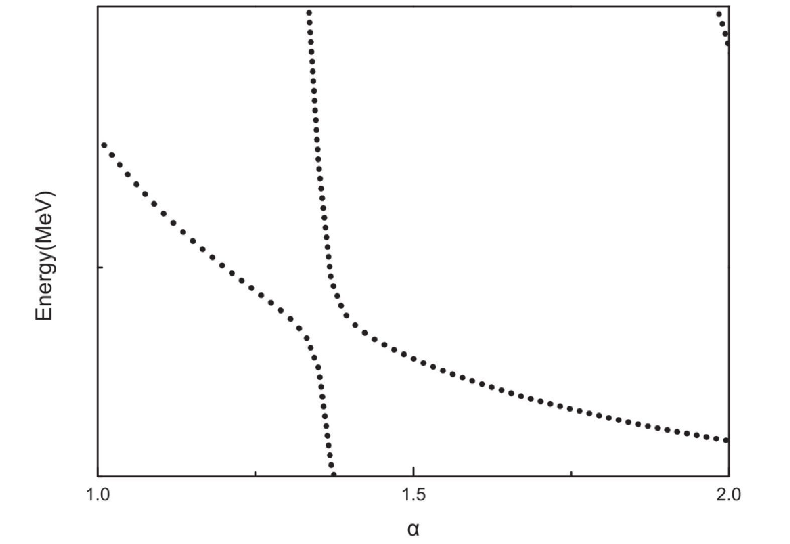
Figure 1. Resonance shape in the real-scaling method.
$ \Gamma = 4 V(\alpha) \frac{ \sqrt{(k_r \times k_c)}} {\lvert k_r-k_c \rvert}. $

(18) $ V(\alpha) $ is the minimal energy difference, while$ k_r $ indicates the slope of the resonance state, and$ k_c $ represents slope of scattering state.The real-scaling results for the positive (Table 4) and negative parity states (Table 5) are illustrated in Figs. 2-6. Here, we only focus on the energy range from
$ 2800 $ to$ 3000 $ MeV because we are interested in the candidates for$ X(2900) $ ; only the$ D^*\bar{K^*} $ threshold is relevant in our calculation, which is marked with a red line. In Fig. 2, the resonance$ E_1(2836) $ rapidly falls to the lowest threshold,$ D\bar{K} $ with the spaces increases, and both$ E_3(2906) $ and$ E_4(2936) $ would decay to the$ D^*\bar{K^*} $ channel. However, the$ E_4(2936) $ may combine with a higher energy level into one avoid-crossing structure, and the structure will be repeated at$ \alpha = 2.2 $ , which indicates the existence of a resonance$ R_0(2914) $ , a possible candidate for$ X_0(2900) $ . In the$ 0^+ $ case, the$ E_4(2936) $ serves as a resonance level, because it has 30% percent of the diquark structure. According to Eq. (18), we estimate its width to be approximately$ 42 $ MeV. In the$ 1^+ $ case (Fig. 3), there are three possible resonances,$ E_7(2904) $ ,$ E_8(2920) $ , and$ E_9(2941) $ , and they all have approximately 30% of the diquark structure. Consequently, the shape of the figure may be very complex. Based on the requirement of the repetitivenes of the avoid-crossing structure, we select one possible resonance,$ R_1(2906) $ . However, the width of$ R_1(2906) $ , which is$ 29 $ MeV, may be unsuitable for$ X_1(2900) $ , which has a width of$ 110 $ MeV.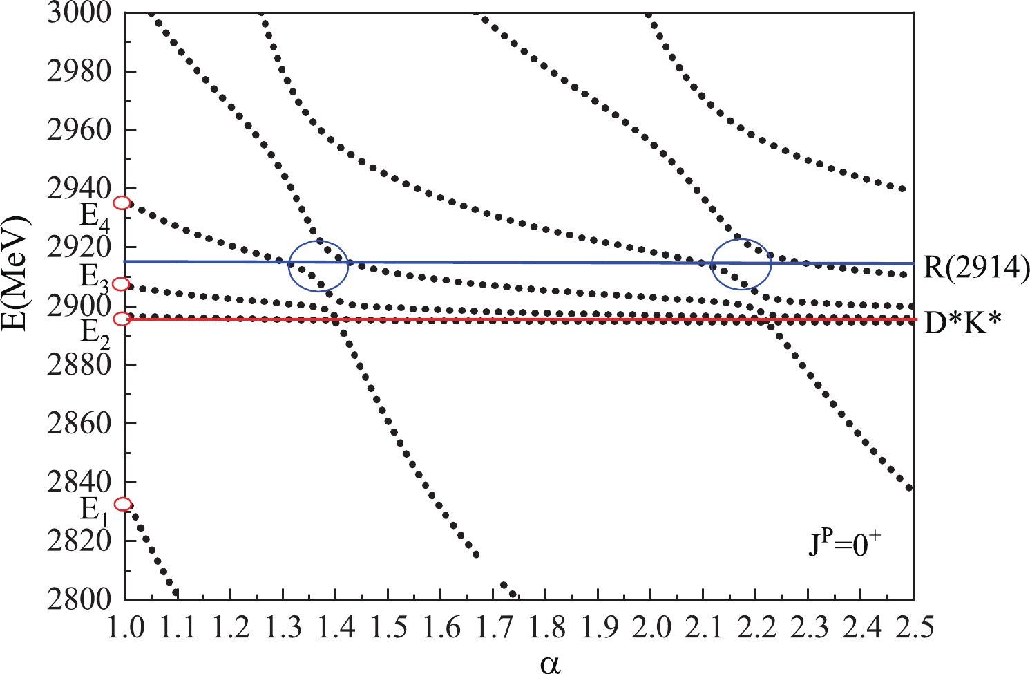
Figure 2. (color online) Energy spectrum of
$^1S_0\; cs\bar{q}\bar{q}$ system.
Figure 4. (color online) Energy spectrum of
$^1P_1\; cs\bar{q}\bar{q}$ system.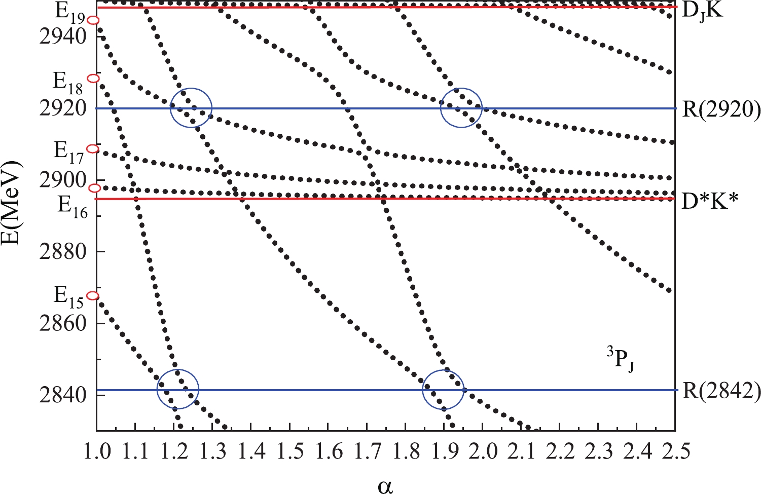
Figure 5. (color online) Energy spectrum of
$^3P_J\; cs\bar{q}\bar{q}$ system.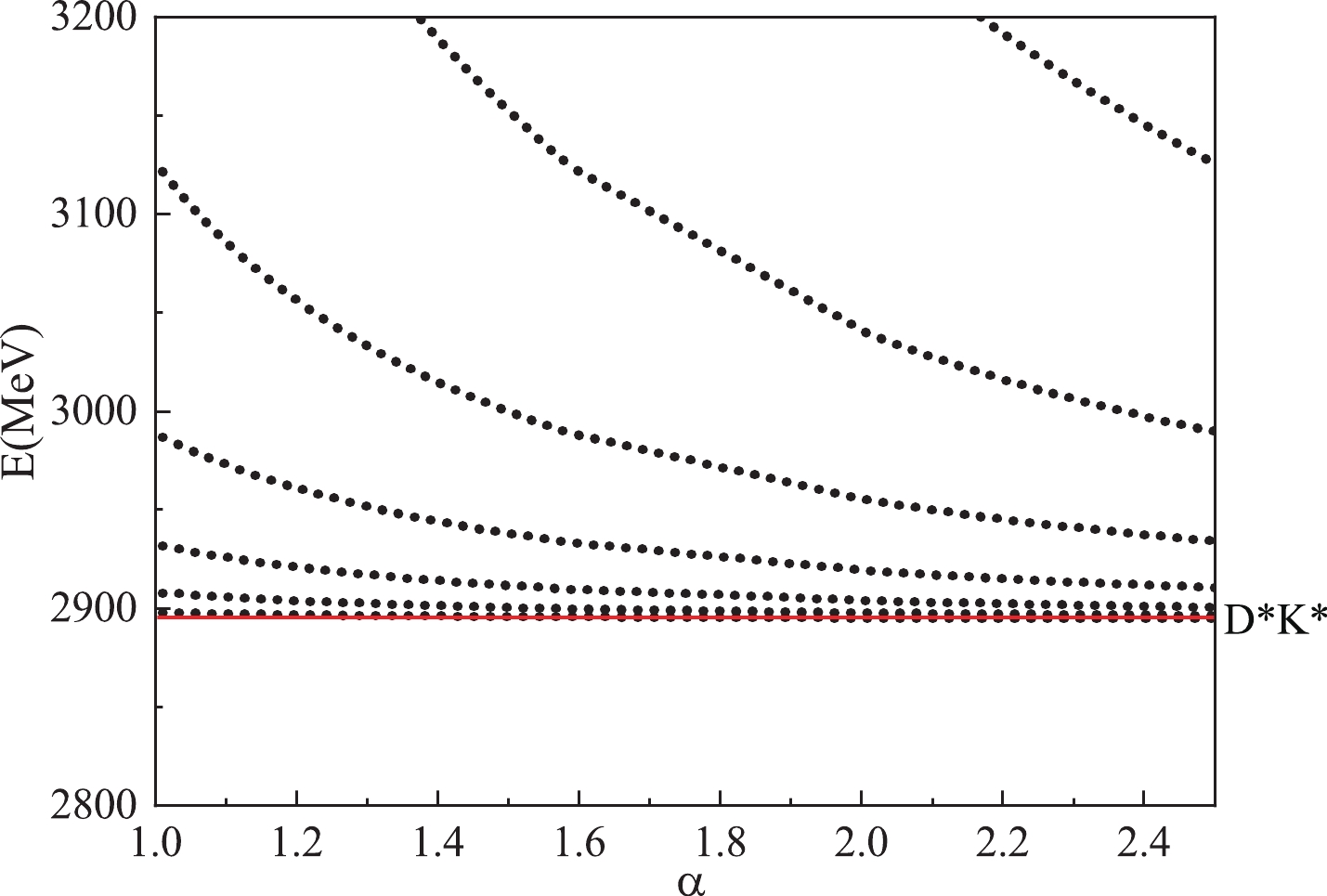
Figure 6. (color online) Energy spectrum of
$^5P_J$ .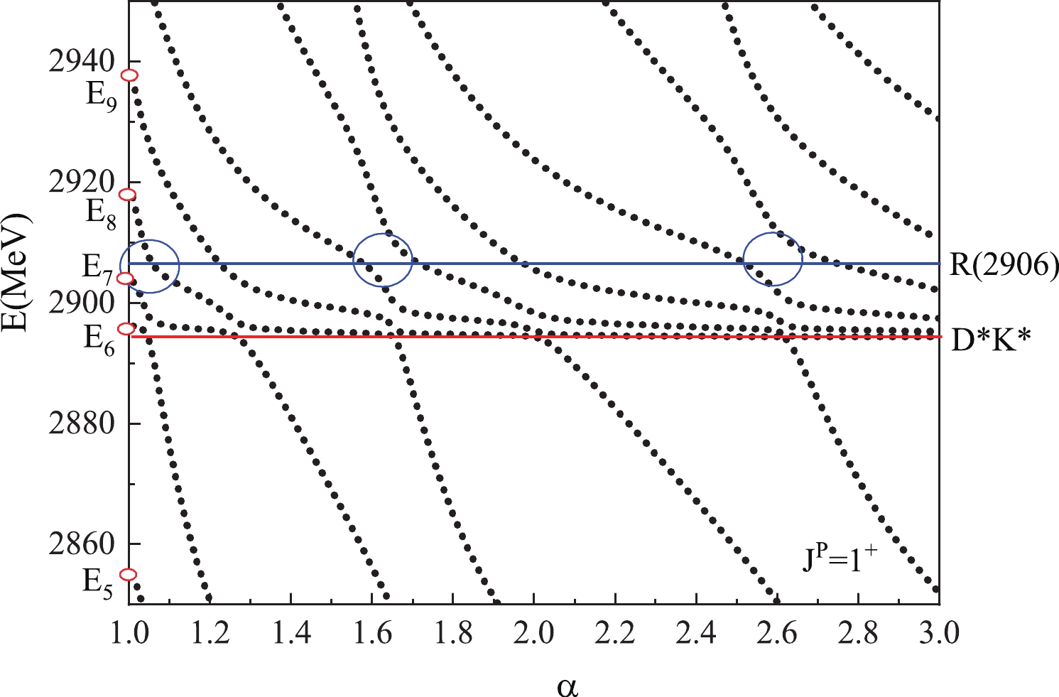
Figure 3. (color online) Energy spectrum of
$^3S_1\; cs\bar{q}\bar{q}$ system.Now, we consider the negative parity states presented in Table 5. Owing to the threshold of the p-wave D meson and K meson close to
$ X(2900) $ , the resonance states may couple to the scattering states strongly, and the pattern may be more complicate. Similar to the$ 00^+\; cs\; \bar{q}\bar{q} $ system, the lines with$ E_{12}(2908) $ ,$ E_{13}(2932) $ fall to the threshold of$ D^*\bar{K^*} $ , and$ E_{14}(2943) $ falls within the threshold of$ D_1\bar{K} $ (see Fig. 4). However, the state$ E_{13}(2932) $ state with 22% of the diquark structure indicates an avoid-crossing structure, which may be a possible resonance,$ R_1(2912) $ with$ \Gamma = 10 $ MeV. Regarding the$ E_{10}(2873) $ state, it rapidly decays to the lower threshold and is not a possible candidate for$ X(2900) $ for the lower energy. Because the$ ^3P_J\; cs\bar{q}\bar{q} $ system has 21 channels including two thresholds near$ X(2900) $ , the pattern of the$ ^3P_J\; cs\bar{q}\bar{q} $ system is very complex. We determine two possible candidates,$ R_J(2920) $ with$ \Gamma = 9 $ MeV and$ R_J(2842) $ with$ \Gamma = 24 $ MeV, for$ X(2900) $ (Fig. 5). Finally, the channels in the$ ^5P_J\; cs\bar{q}\bar{q} $ system have higher energies than$ X(2900) $ , and$ D^*\bar{K}^* $ is a p-wave excited scattering state. From the figure, it can be observed that no resonance survives the coupling to the p-wave scattering state (see Fig. 6). Although the energies of the above resonance states with negative parity are close to the mass of$ X_1(2900) $ , the larger width of$ X_1(2900) $ prevents the formation of a conclusion. -
In the framework of the chiral constituent quark model, we systematically studied
$ cs\bar{q}\bar{q} $ states to determine the candidates for$ X(2900) $ , which were reported by the LHCb Collaboration recently. Both the molecular structure, as well as the diquark-antidiquark, with all the possible color, flavor, and spin configurations are considered in the present calculation. The obtained results indicate that there are several states with energies of approximately 2900 MeV in the$ cs\bar{q}\bar{q} $ system after structure-mixing. These superabundant resonances may be triggered by the structure mixing and finite calculation space. Therefore, the real-scaling method, a stablization method, is adopted to identify the genuine resonances. We obtained five possible resonances,$ R_0(2914) $ with$ \Gamma = 42 $ MeV,$ R_1(2906) $ with$ \Gamma = 29 $ MeV,$ R_1(2912) $ with$ \Gamma = 10 $ MeV,$ R_J(2920) $ with$ \Gamma = 9 $ MeV, and$ R_J(2842) $ with$ \Gamma = 24 $ MeV. All the resonances obtained are diquark-antidiquark states. For$ X_0(2900) $ , the resonance,$ R_0(2904) $ with$ \Gamma = 42 $ MeV, may be a good candidate. In this case,$ X_0(2900) $ would be the positive parity state. However, it is possible to assign candidates for$ X_1(2900) $ based on energy, but the decay width prevent us from making a definite conclusion. Hence, more information on$ X(2900) $ and further studies are required.
X(2900) in a chiral quark model
- Received Date: 2021-04-12
- Available Online: 2021-09-15
Abstract: Recently, the LHCb Collaboration reported their observation of the first two fully open-flavor tetraquark states named


 DownLoad: