


 Abstract
 HTML
HTML Reference
 Related
 PDF
PDF


-
The increase in number of meson and baryon resonances that have been added to the Particle Data Group (PDG) [1] has stimulated research for a better understanding of the excited hadron spectrum. The quark model describes these resonances as radial and orbital excitations; however, the number of observed resonances awaiting classification has increased. Significant efforts have been made toward searching for a complete description of the quantum numbers, masses, dimensions, and other properties of the resonances. Examples of such efforts are the ab initio quantum chromodynamic (QCD) calculation of the mass spectra of light hadrons [2], lattice QCD calculation of the N and ∆ baryon mass spectra [3], calculation of the excited states of selected mesons [4, 5], hypercentral constituent quark model calculation of the N resonances [6], calculation of Ωccc and Ωbbb using the orbital and radial Regge trajectories [7], and relativistic quark model calculation of the properties of light, light-heavy, and heavy-heavy mesons based on Regge trajectories [8-10]. In 1966, Pauling noticed that more than half of the baryon resonances could be described as rotational states of a semi-rigid rotor [11]. By interpreting the orbital resonances of the Δ baryon as excited states of a three-quark spin quartet with a trigonal planar configuration rotating about an axis that is normal to the symmetry axis, Pauling’s calculations agreed within the experimental uncertainty. Subsequently, a constituent quark model calculation, which incorporated the rigid rotor and the harmonic oscillator, yielded the mass spectra with some experimental correlation; however, the resulting radial quantum numbers were larger than those predicted using the quark model [12, 13]. The rigid rotor was also used in the chiral quark-soliton model because the quantization of the soliton rotation is similar to the quantization of the spherical rigid rotor [14, 15]. By contrast, the harmonic oscillator potential has been widely used to describe the radial excitations of mesons and baryons [16, 17], although it becomes less reliable for the higher radial quantum numbers [18]. However, the anharmonic correction and deformed harmonic oscillator can provide an improved description of the resonances for the nucleons and Δ baryon [19-21]. In this paper, we present a rovibrational model, which incorporates the semi-rigid rotor as well as the anharmonic and Coriolis corrections to describe the radial and orbital resonances of the π, K, N, and Ʃ hadrons. The calculated results were found to be in good agreement with those of the experimental and other theoretical studies. This model allows for the classification as well as prediction of the resonances, being useful for understanding the excited spectra of these hadrons. The details of the rovibrational model are described in the next section.
-
In case of π and K mesons, the quark and antiquark, separated by a distance r and having opposite spins, occupy s orbitals. In N and Ʃ baryons, the three quarks, two with opposite spins, occupy s orbitals centered on the vertices of a triangle, corresponding to a symmetrical top oblate structure. The vibration of the quarks and the rotation of these particles can be described by the stationary Schrödinger equation with Morse potential, which considers the anharmonic and semi-rigid rotor corrections [22]. The angular solution, similar to the hydrogen atom, is the well-known
$ {Y}_{l}^{m}\left(\varTheta ,\phi \right) $ =$ \varTheta \left(\theta \right)\varPhi \left(\phi \right) $ spherical harmonics. The radial equation is given as follows:$\begin{aligned}[b] \frac{{\rm d}^{2}R\left(r\right)}{{\rm d}{r}^{2}}+\frac{J\left(J+1\right)R\left(r\right)}{{r}^{2}}=&\frac{-8{\pi }^{2}m}{{h}^{2}}\left[E-D-D{\rm e}^{-2\alpha \left(r-{r}_{e}\right)}\right.\\&\left.+2D{\rm e}^{-\alpha \left(r-{r}_{e}\right)}\right]R\left(r\right), \end{aligned}$

(1) where R(r) is the radial wave function, J is the orbital quantum number, m is the mass of the particle, h is the Planck’s constant, E is the total energy,
$ D+ D{\rm e}^{-2\alpha \left(r-{r}_{e}\right)}- $ $ 2D{\rm e}^{-\alpha \left(r-{r}_{e}\right)} $ is the Morse potential, r is the equilibrium distance, D and$ \alpha $ are parameters characteristic to each particle. For molecules, the Morse potential allows the escape of the vibrating objects into the continuum, and D corresponds to the dissociation energy. This does not happen for confined quarks. The Morse potential will be used here to describe only the excited spectrum of hadrons and not to calculate the effective potential of the quarks. Eq. (1) can be solved numerically; however, an analytical solution allows to separately identify the contribution of each term of the rovibrational energy. Using the Pekeris solution [23], which includes the rovibrational coupling for states with J > 0, the masses of the resonances$ M(n,J) $ can be calculated as (in MeV)$ \begin{aligned}[b] M(n,J)=&D+\hslash \omega \left(n+\frac{1}{2}\right)-\hslash \omega {x}_{e}{\left(n+\frac{1}{2}\right)}^{2}\\&+{B}_{\rm rot}J\left(J+1\right)-{D}_{\rm rot}{J}^{2}{\left(J+1\right)}^{2} \\ &-{\alpha }_{e}\left(n+\frac{1}{2}\right)J\left(J+1\right), \end{aligned} $

(2) where n is the radial quantum number,
$ \hslash \omega \left(n+\dfrac{1}{2}\right) $ represents the harmonic contribution,$ \hslash \omega {x}_{e}{\left(n+\dfrac{1}{2}\right)}^{2} $ is the anharmonic correction,$ {B}_{\rm rot}J\left(J+1\right) $ is the rigid rotor contribution,$ {D}_{\rm rot}{J}^{2}{\left(J+1\right)}^{2} $ represents the semi-rigid rotor correction, and the rovibrational coupling is given by$ {\alpha }_{e}\left(n+\dfrac{1}{2}\right)J\left(J+1\right) $ , which is the so-called Coriolis effect. The parameter$ {B}_{\rm rot}=\dfrac{{\hslash }^{2}}{2I} $ with$ I=m{r}^{2} $ was previously determined using the experimental mass and radius of the reference particle. For this reason, in this study, we selected π+, K+, N+, and Σ−, which have well-defined charge radii and masses. The charge radius,$ {r}_{E} $ , is taken as the distance between the quarks. For mesons,$ r=\dfrac{{r}_{E}}{2} $ , and for baryons,$ r=\dfrac{{r}_{E}}{\sqrt{3}} $ . D and the coefficients$ \hslash \omega $ ,$ \hslash \omega {x}_{e} $ ,$ {D}_{\rm rot} $ , and$ {\alpha }_{e} $ are obtained by fitting the resonance masses as a function of the radial and orbital quantum numbers (Eq. (2)). The particle masses, charge radii,${J}^{P} $ , and rovibrational parameters of π+, K+, N+, and Σ− hadrons are listed in Table 1.Particle $ {r}_{E}\,{\rm{/fm}} $ 

$ {J}^{P} $ 

$ {m}_{\rm part} \,{\rm{/MeV}} $ 

D/MeV $ \hslash \omega\,{\rm{/MeV}} $ 

$ \hslash \omega {x}_{e}\,{\rm{/MeV}} $ 

$ {B}_{\rm rot} \,{\rm{/MeV}} $ 

$ {D}_{\rm rot}\,{\rm{/MeV}} $ 

$ {\alpha }_{e} \,{\rm{/MeV}} $ 

π+ 0.659 0− 139.57±1.8×10⁻⁴ 725.58 464.98 22.34 1284.81 3.57 2298.17 K+ 0.560 0− 493.68±1.6×10⁻² 575.41 732.50 85.22 503.02 4.70 660.93 N+ 0.875 1/2+ 938.27±6.0×10⁻⁶ 1071.16 309.64 4.62 81.30 0.78 32.07 Ʃ− 0.780 1/2+ 1197.45±3.0×10⁻² 1361.01 197.76 12.13 80.18 1.28 32.94 Table 1. Charge radii,
${J}^{P} $ , masses, and rovibrational parameters of π+, K+, N+, and Ʃ− hadronsThe behavior of the rovibrational parameters is similar to that of the molecules, although the corrections are significantly higher for the hadrons. The harmonic contribution is the largest, for both molecules and hadrons, except for π, which has a small mass and a large rotational energy. In general, the Coriolis effect is smaller than the vibrational and rotational contributions, except for π and K, which have small masses and charge radii. Higher Brot values are observed for mesons as compared to the baryons. For J = 0, there is no Coriolis effect. However, for J > 0, which is the case for the majority of the hadrons, this effect becomes significant.
A comparison of the calculated rovibrational states with the experimental and other theoretical results is discussed in the next section.
-
Table 2 compares the calculated π, K, N, and Ʃ orbital resonances with those obtained from the experiments and other theoretical predictions.
Hadron Resonance JPC/JP Status Mass Ref. Exp. This work Others π b(1235) 1+− • 1229.5±3.2 1210 1302 [24] π2(1670) 2−+ • $ {1670.6}_{-1.0}^{+2.9} $ 

1638 1666 b3(2030) 3+− f. 2032±12 2068 1972 π4(2250) 4−+ f. 2250±15 2240 2242 K K1(1270) 1+ • 1253±7 1247 1272 [25, 26] K2(1770) 2− • 1773±8 1787 1758 K3(2320) 3+ 2324±24 2315 2303 K4(2500) 4− 2490±20 2492 2498 N N(1520) 3/2− **** 1515±5 1459 1535, 1537, 1542 [6, 18, 27] N(1680) 5/2+ **** 1685±5 1736 1660, 1769, 1799 N(2190) 7/2− **** 2180±40 2060 2045, 2150 N(2220) 9/2+ **** 2250±50 2365 2183 N(2600) 11/2− *** $ {2600}_{-50}^{+150} $ 

2566 2687 ∑ ∑(1670) 3/2− **** 1675±10 1678 1680, 1800 [27, 18] ∑(1915) 5/2+ **** $ {1915}_{-15}^{+20} $ 

1916 1901, 2041 ∑(2100) 7/2− * 2146±17 2143 ∑(2250) 9/2+ *** 2250±30 2251 Table 2. Experimental and calculated π, K, N, and Ʃ orbital resonances. Fourth column indicates the resonance status assigned by the PDG. The states indicated with “•”, “***,” and “****” are well-established, while those indicated with a blank space, “f.,” “*,” and “**” are awaiting confirmation. Mesons indicated with “f.” are listed in the "other states" section of the PDG. The state emphasized in bold font indicates a resonance without confirmed JP.
The selected resonances of each family have the same spin s, isospin I, dimensionality (baryons), and quark flavors. These resonances obey the classification of the quark model and the criterion of naturality and parity. The resonances of the π and K mesons, both with JP = 0- and n = 0, have unnatural spin–parity. The N and Σ baryon resonances, with
$J^P$ = 1/2+ and n = 0, have natural spin-parity. Table 2 indicates that the observed and calculated values are well correlated. They also agree with other theoretical predictions obtained using Regge trajectories [6, 24-26]. The π orbital excitations are associated with the resonances b(1235), π2(1670), b3(2030), and π4(2250); the last two are listed as “Further States” in the PDG. Orbital Regge trajectory calculations lead to this same grouping [6, 24-28]. The K orbital excitations are associated with resonances K1(1270), K2(1770), K3(2320), and K4(2500). Regge trajectories in quadratic form (m2 = β (cll + πnr + c0)2/3 + c1) using the spinless Salpeter-type equation [25, 26] classifies K2(1770) as a 11D2 state, suggesting that it is an orbital and excitation of the K meson. The rovibrational model gives m = 1787 MeV with J = 2– and n = 0 for this resonance, which is in agreement with that classification. The first five N orbital excitations are (70,$ {1}_{1}^{-} $ ), (56,$ {2}_{2}^{+} $ ), (70,$ {3}_{3}^{-} $ ), (56,$ {4}_{4}^{+} $ ), and (70,$ {5}_{5}^{-} $ ) states [1, 29], which are in agreement with the grouping of the resonances N(1520), N(1680), N(2190), N(2220), and N(2600) reported in this paper. A constituent quark model that uses the Regge trajectory classifies the three resonances N(1520), N(1680), and N(2190) as 1P, 1D, and 1F states, respectively [6, 30]. This classification also corroborates the results reported here. The Ʃ family, where there is a very good experimental agreement, includes the three well-established resonances Ʃ(1670), Ʃ(1915), and Ʃ(2100). The quark model classifies only the first two resonances as the (70,$ {1}_{1}^{-} $ ) and (56,$ {2}_{2}^{+} $ ) states. Here, the resonance Ʃ(2100) with J = 7/2– appears to be the candidate for the (70,$ {3}_{3}^{-} $ ) state, which is in agreement with Regge phenomenology [31]. Currently, this baryon has eight resonances without$J^P $ . Here, the Ʃ(2250) resonance is identified as the orbital excitation with m = 2251 MeV and$J^P $ = 9/2+.Table 3 compares the π, K, N, and Σ radial resonances that are calculated using the rovibrational model with those observed experimentally and predicted by other theories. Table 3 evidently indicates that the calculated masses are in good agreement with the experimental data. The radial excited states of π are identified as the resonances π(1300), π(1800), π(2070), π(2360), and π(2610). The first two resonances correspond to 21S0 and 31S0 states, as described by the quark model. Regge trajectory groupings also include these two π resonances [25, 26, 30]. The resonances π(2070) and π(2360), observed approximately 20 years ago, are listed in the "Further states" section of the PDG. The π radial family is expected to contain the resonance with m = 2607 MeV, corresponding to the 61S0 state. The first K radial excitation is associated with the resonance K(1460), which is described as the 21S0 state by the quark model. The 31S0 state, i.e., the second radial excitation, corresponds to the resonance K(1830) in agreement with the Regge trajectory calculations [25, 26]. The 41S0 state with m = 2095 MeV is predicted as the third K radial excitation. The N radial excitations correspond to the four known resonances, N(1440), N(1880), N(2100), and N(2300). The modified Regge trajectories that are based on the holography inspired stringy hadron (HISH) model corroborate the classification of N(1880) resonance in the N family [30]. Moreover, Klempt and Richard [29] classified the N(1880) resonance as a state (70,
$ {2}_{2}^{+} $ ), suggesting that it corresponds to the N radial excitation second. Shah [6] associated the N(2100) resonance to the 4S state and predicted the 5S state with m = 2515 MeV, neglecting the N(2300) resonance. However, the rovibrational model satisfactorily accommodates N(2300) after N(2100) resonance in the N family as 4S and 5S states, respectively. In addition, it also predicts the 6S state with n = 5,$J^P $ = 1/2+, and m = 2563 MeV. The resonances Ʃ(1660), Ʃ(1770), and Ʃ(1880) are associated with the first three Ʃ radial excitations, in agreement with the relativistic interacting quark-diquark model [27]. In the PDG, the state (70,$ {0}_{2}^{+} $ ) is associated with the Ʃ(1880) resonance, whereas Klempt and Richard [29] associated this state with the Ʃ(1770) resonance. The present results indicate that Ʃ(1770) and Ʃ(1880) belong to the same Ʃ radial family, with n = 2 and n = 3, respectively. The rovibrational model also suggests a new radial resonance with$J^P $ = 1/2+ and m = 1954 MeV.Hadron Resonance n Status Mass Ref. Exp. This work Others π π(1300) 1 • 1300±100 1373 1292 [8] π(1800) 2 • $ {1810}_{-11}^{+9} $ 

1748 1788 π(2070) 3 f. 2070±35 2079 π(2360) 4 f. 2360±25 2366 π(2610) 5 p. 2607 K K(1460) 1 1482.4±3.58 1482 1464 [25, 26] K(1830) 2 1874±43 1874 1829 K(2100) 3 p. 2095 N N(1440) 1 **** 1440±30 1550 1425, 1511 [6, 14, 27] N(1880) 2 *** 1880±50 1817 1890 N(2100) 3 *** 2100±50 2075 2089 N(2300) 4 ** $ {2300}_{-30}^{+40} $ 

2323 N(2560) 5 p. 2563 ∑ Ʃ(1660) 1 *** 1660±20 1653 1734 [14] Ʃ(1770) 2 * 1770±20 1777 1739 Ʃ(1880) 3 ** 1880±60 1878 1751 Ʃ(1950) 4 p. 1954 Table 3. Experimental and calculated π, K, N, and Σ radial resonances. “p.” indicates predicted states.
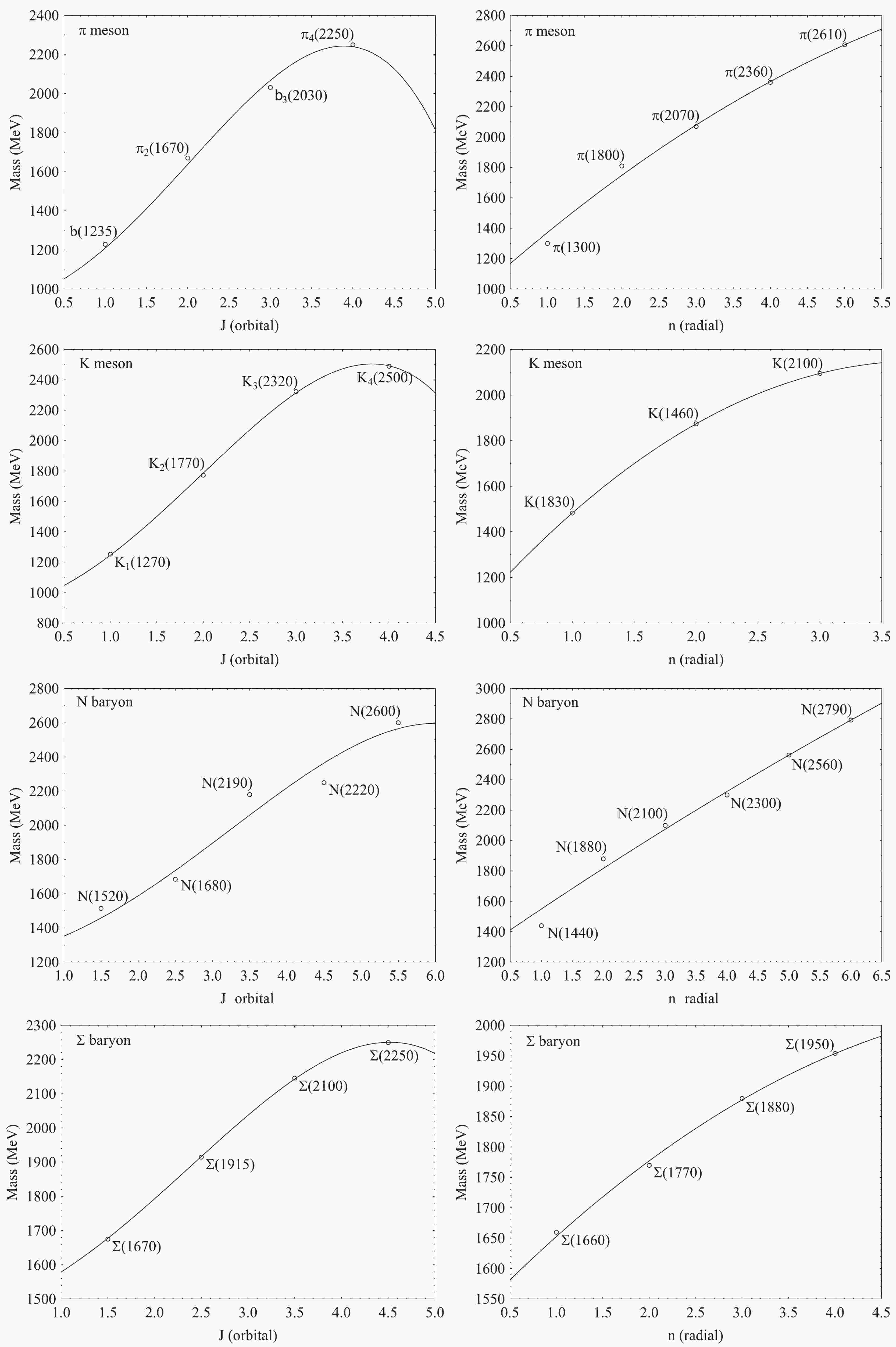
Linear Regge trajectories have been used for describing the resonances of mesons and baryons [6, 30]; however, a non-linear behavior of the masses of the orbital and radial resonances have been reported [25, 26, 28, 31, 32]. A study on the concavity of the Regge orbital and radial meson trajectories have concluded that they can be concave or convex [25, 26]. Recently, a non-linear Regge trajectory, expressed as J = c + d((-m)2)1/2 was used to calculate the spectrum of the N, ∆, Ʃ, and Λ resonances [9, 14]. Figure 1 shows the nonlinear behavior of the π, K, N, and Ʃ radial and orbital excitations, as calculated by the rovibrational model.

Figure 1. Fitted curves of the π, K, N, and Ʃ orbital (m, J) and radial (m, n) resonances calculated by the rovibrational model.
Figure 1 shows the curves in good agreement with the experimental data. The corrections included in this model, such as those of anharmonicity, centrifugal distortion, and Coriolis coupling, are crucial for obtaining masses that are close to the experimental values and follow a nonlinear behavior. The curves (m, J) and (m, n) indicate that the mass increases with the orbital number J or the radial number n, as has been observed, but they also exhibit a maximum in the curves. However, taking into account that Pekeris' approximate solution neglects higher order terms, the downward parts of the curves may reflect the limit of Eq. (2).
-
The proposed rovibrational model proved to be useful in classifying the π, K, N, and Ʃ radial and orbital resonances. The four J excited states of the π meson are associated with the orbital resonances b(1235), π2(1670), b3(2030), and π4(2250). Its radial excited states correspond to the resonances π(1300), π(1800), π(2070), and π(2360). In the K family, the four orbital excitations are associated with the resonances K1(1270), K2(1770), K3(2320), and K4(2500). The first and second radial excitations of K are associated with the resonances K(1460) and K(1830), respectively. Further, the K meson is expected to have a resonance with m = 2095 MeV, corresponding to the third K radial excitation. The N orbital excited states are associated with the resonances N(1520), N(1680), N(2190), N(2220), and N(2600), whereas the first four N radial excitations are associated with the N(1440), N(1880), N(2100), and N(2300) resonances. Moreover, this model predicts the existence of another resonance state with m = 2563 MeV, n = 5, and
$J^P $ = 1/2+. The Ʃ family includes the four orbital resonances Ʃ(1670), Ʃ(1915), Ʃ(2100), and Ʃ(2250). This last resonance is associated with the orbital excitation with$J^P $ = 9/2+. The first three Ʃ radial excitations correspond to the resonances Ʃ(1660), Ʃ(1770), and Ʃ(1880). The rovibrational model predicts a new radial resonance with$J^P $ = 1/2+ and m = 1954 MeV.In conclusion, the rovibrational model is useful for classifying the hadron resonances, leading to a good agreement with the experimental observations and predicting new hadron resonances. The next step is to apply the model to study other hadrons.
Hadron resonances as rovibrational states
- Received Date: 2020-03-09
- Available Online: 2021-08-15
Abstract: A rovibrational model, including anharmonic, centrifugal, and Coriolis corrections, is used to calculate π, K, N, and Ʃ orbital and radial resonances. The four orbital excitations of the π meson correspond to the b(1235), π2(1670), b3(2030), and π4(2250) resonances. Its first four radial excitations correspond to the π(1300), π(1800), π(2070), and π(2360) resonances. The orbital excitations of the K meson are interpreted as the K1(1270), K2(1770), K3(2320), and K4(2500) resonances; its radial excitations correspond to the K(1460) and K(1830) resonances. The N orbital excitations are identified with the N(1520), N(1680), N(2190), N(2220), and N(2600) resonances. The first four radial excitations of the N family correspond to the N(1440), N(1880), N(2100), and N(2300) resonances. The orbital excitations of the Ʃ baryon are associated with the Ʃ(1670), Ʃ(1915), Ʃ(2100), and Ʃ(2250) resonances, whereas its radial excitations are identified with the Ʃ(1660), Ʃ(1770), and Ʃ(1880) resonances. The proposed rovibrational model calculations show a good agreement with the corresponding experimental values and allow for the prediction of hadron resonances, thereby proving to be useful for the interpretation of excited hadron spectra.


 DownLoad: