


 Abstract
 HTML
HTML Reference
 Related
 PDF
PDF


-
The nature of dark matter (DM) remains an intriguing physics question today. The direct search for an important class of dark matter candidate, the weakly interacting massive particles (WIMPs), has been accelerated by development in dual phase xenon time projection chambers (TPCs), such as PandaX-II [1], XENON-1T [2], and LUX [3]. In these detectors, a WIMP may interact with xenon nuclei via elastic scattering, depositing a nuclear recoil (NR) energy from few keVnr to a few tens of keVnr. γs or βs from internal impurities. The detector materials produce electron recoil (ER) background events with insignificant probabilities identified as the NR signals.
In a dual phase xenon TPC bounded by a cathode at the bottom in the liquid and an anode at the top in the gas, each energy deposition is converted into two channels, the scintillation photons and ionized electrons. The former is the so-called S1 signal. Electrons are subsequently drifted towards the liquid surface, and extracted into the gas region with delayed electroluminescence photons (S2) produced. Both S1s and S2s are collected by two arrays of photomultiplier tubes (PMTs) located at the top and bottom of the TPC. For a given event, the combination of S1 and S2 allows the reconstruction of the recoil energy and vertex, and the proportion of S1 and S2 serves as a significant discriminant for ER and NR. It is essential to determine the detector response via in situ calibration.
For the ER response, the injected sources used in PandaX-II, include tritiated methane (CH3T), 220Rn, and
$ ^{83{\rm{m}}}{\rm{Kr}} $ . For NR calibration, an external 241Am-Be (AmBe) neutron source was used. In this study, the detector responses are determined by fitting these data under the NEST2.0 [4] prescription.The rest of this paper is organized as follows. In Sec. II, the detector conditions and calibration setups are introduced. In Sec. III, data processing and event selection cuts are presented. The response model simulation will be introduced in Sec. IV, followed by detailed discussions on the fits of the light yield and charge yield, before the conclusion in Sec. V.
-
The PandaX-II experiment, located at the China Jinping underground laboratory (CJPL) [5], was under operation from March 2016 to July 2019, with a total exposure of 132 ton
$ \cdot $ day for dark matter search. The operation was partitioned into three runs, Runs 9, 10, and 11 [6], with calibration runs interleaved in between. The detector contained 580-kg liquid xenon in its sensitive volume. The liquid xenon was continuously purified through two circulation loops, each connected to a getter purifier. The internal ER sources were injected through some loop. Two PTFE tubes, at 1/4 and 3/4 height of the TPC surrounding the inner cryostat, were used as the guide tube for the external AmBe source. The TPC drift field in Run 9 was 400 and 317 V/cm in Runs 10/11, corresponding to the maximum drift times 350, and 360 μs, respectively. The running conditions, key detector parameters, and event selection ranges for the calibration data sets are presented in Table 1.Data set Run9 AmBe Run9 Tritium Runs 10/11 AmBe Runs 10/11 220Rn PDE 0.115±0.002 0.120±0.005 EEE 0.463±0.014 0.475±0.020 SEG 24.4±0.4 23.5±0.8 $E_{\rm{drift}}$ /(V/cm)

400 317 $E_{\rm{extract}}$ /(kV/cm)

4.56 Livetime/d 6.7 27.9 48.5 11.9 Number of events 2902 9387 11196 8841 Drift time cut/ $\mu{\rm s}$ 

18-200 18-310 50-200 50-350 range cut S1:3-150 PE S2:100-20000 PE $E_{\rm{rec}}<25$ keV

S1:3-150 PE S2:100-20000 PE $E_{\rm{rec}}<25$ keV

Table 1. Summary of ER and NR calibration data sets and corresponding detector configurations. PDE, EEE, and SEG, respectively, are the photon detection efficiency, electron extraction efficiency, and single electron gain. The values and systematics uncertainties are from Ref. [6].
$E_{\rm{drift}}$ and$E_{\rm{extract}}$ are the drift field and extraction field. The number of events correspond to the calibration data after all cuts, which are described in Sec. III. -
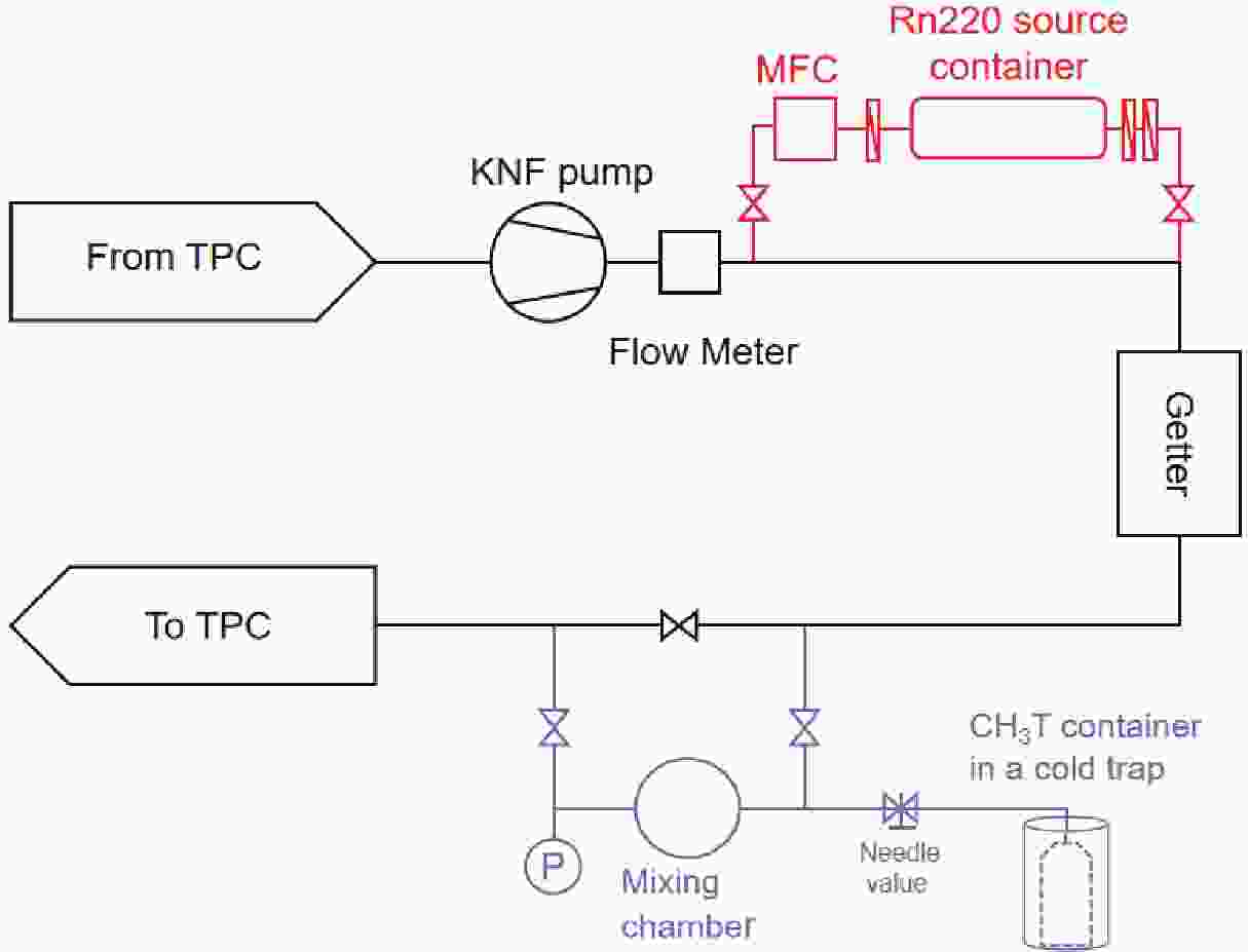
Tritiated methane calibration was initially developed by a LUX experiment [7] and recorded an excellent internal low energy β events. The tritiated methane source used in the PandaX-II was procured from American Radio labeled Chemicals, Inc., with a specific activity of 0.1 Curie per mole of methane. The injection diagram is shown in Fig. 1. The tritiated methane bottle was immersed in a liquid-nitrogen cold trap, so that a controllable quantity of CH3T gas can diffuse through a needle valve to the 100 mL mixing volume. The gas in the mixing volume was flushed with xenon gas into the detector.
Figure 1. (color online) Tritiated methane (blue) and 220Rn (red) injection system. Tritiated methane injection system is installed downstream of the purifier to prevent chemical attachment to the purifier before entering into TPC.
The injection of tritium was performed in 2016 after Run 9, wherein approximately 5.4
$ \times 10^{-10} $ mol of methane was loaded into the detector. The tritium events were distributed uniformly in the detector. Liquid xenon was constantly circulated at approximately 40 SLPM (standard liter of gas per minute) through the purifier. The duration for the calibration run was 44 days, and the later data set with an average electron lifetime of 706 μs is used as the ER calibration data.We observed that the hot getters were inefficient to remove tritium with activity plateau at 10.2 μBq/kg. We performed an offline distillation campaign after the calibration to reduced the tritium activity to 0.049±0.005 μBq/kg in Runs 10/11 [6].
-
220Rn, a decay progeny of 232Th, is a naturally occurring radioactive noble gas isotope. Because its half-life is 55 s, the probability to contaminate the liquid xenon TPC is insignificant, as initially demonstrated in XENON100 [8]. Details of 220Rn calibration setup and operation in PandaX-II is presented in Ref. [9]. The injection system consisting of a mass flow controller and a 232Th source chamber with filters upstream and downstream, is shown in Fig. 1. In this injection, lantern mantles treated with thorium nitrate (
$ {\rm{Th(NO_3)_4}} $ ) were used as the radon sources that gives a rate of 31.7 ± 0.3 Bq 220Rn decays in the FV (define later in Sec. III). After 220Rn was injected into the detector, the β-decay of the daughter nucleus 212Pb gives uniformly distributed ER events with energy extending to zero. 11.9 days of 220Rn data in 2018 are used as the low energy ER calibration for Runs 10/11. -
Neutron calibration data with an AmBe (α, n) source [10] with an approximate neutron emission rate of 2 Hz, producing an approximate 400 low energy nuclear recoils in the FV per day, were considered in Run 9 and Runs 10/11. The source was placed in the external calibration tubes. Calibration runs were recorded at eight symmetric locations in each loop to evenly sample the detector. For different source locations, no significant difference is identified in the detector response, therefore, we grouped the data in the analysis.
-
The processing of the calibration data follows the procedure in Ref. [6]. Compared to the analyses [1, 11], seven unstable PMTs are inhibited from all data sets for consistency. This enhanced the PMT gain calibration, quality cuts, position reconstruction, and corresponding non-uniformity correction.
The raw S1 and S2 of each event is initially corrected for position non-uniformity based on the three-dimensional variation of the raw S1 and S2 for the uniformly distributed mono-energetic events, e.g. 164 keV (
$ ^{131{\rm{m}}} {\rm{Xe}}$ ) owing to activation from the neutron source. The correction to S1 is a smooth three-dimensional hyper-surface. The correction to S2 is separated into an exponential attenuation vs. drift time (electron lifetime τ), and a smooth two-dimensional surface in the horizontal plane.The electron equivalent energy of each event is reconstructed by
$ E_{\rm{rec}} = W \times \left(\frac{S1}{{\rm{PDE}}}+\frac{S2}{{\rm{EEE}}\times{\rm{SEG}}}\right), $

(1) where
$ W = 13.7 $ eV [12] is the average energy to produce either a scintillation photon or free electron in liquid xenon, and PDE, EEE, and SEG, respectively, are the photon detection efficiency (ratio of detected photoelectrons to the total photons), electron extraction efficiency, and single electron gain, from the data (see Ref. [6] and Table 1). Recently, there is a new measurement of W in liquid xenon [13], yielding W =$ 11.5\pm0.5 $ eV, however, we used approximately 16% less. If we adopted the new value, the PDE and EEE will increase by 16%, although the main effect in the response model in (S1, S2) will be scaled out.Events with a single pair of S1 and S2 are selected. The fiducial volume (FV) definition is consistent with Ref. [6], except that a lower cut in drift time (200 μs) is applied to the AmBe data to prevent events that multi-scatter and deposit part of the energy in the below-cathode region, leading to suppressed S2 [11]. The lower selection cuts
$ S1>3 $ PE and$ S2_{\rm{raw}}>100 $ PE are applied to all data sets. For the AmBe data, the upper selection cut is set at$ S1<150 $ PE ($ \sim 80$ keVnr). For ER data, events with$ E_{\rm{rec}}<25 $ keV are selected. The vertex distributions of selected events are shown in Fig. 2, with FV cuts indicated. For all run sets, the bright bands at the maximum drift time (corresponding to cathode background) is constant at different radii. This is consistent with our COMSOL [14] simulation that predicts a better than 1% field uniformity throughout the FV. Therefore, in all later detector models, no field non-uniformity is considered.
Figure 2. (color online) Event vertex distribution in drift time vs. radius-squared for each calibration data set. The FV region is indicated by dashed red line in each figure.
The distributions of S2 vs. S1 for ER and NR events shown in Fig. 3 are used to determine the detector response model.
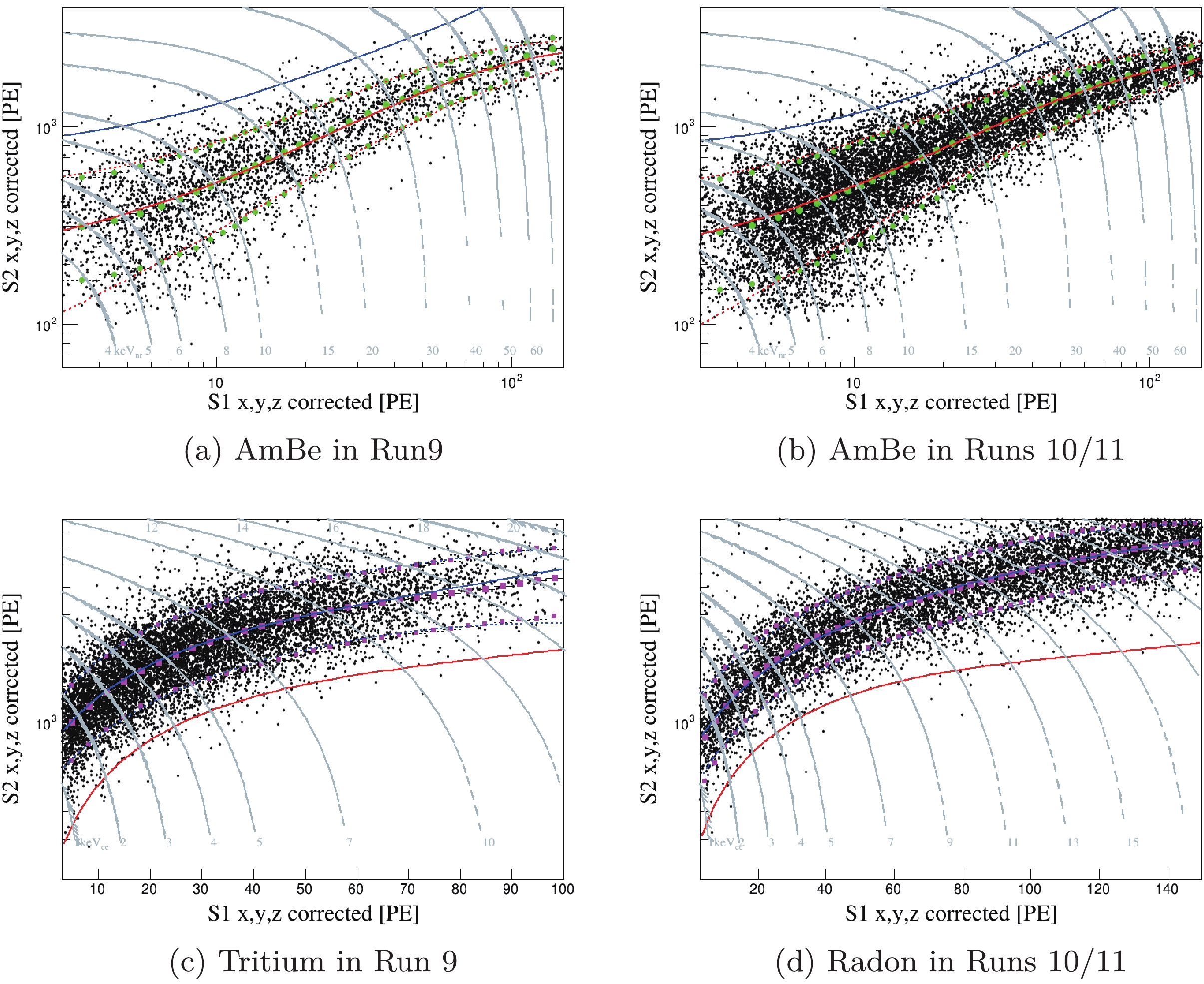
Figure 3. (color online) S2 vs. S1 of the selected calibration events. The red (blue) solid lines are the medians of NR (ER), and the red (blue) dashed lines refer to the 90% quantiles. For comparison, the 90% quantiles from the best fit response models (Sec. IV) are overlaid as the green (purple) dotted lines for NR (ER). The gray dashed curves are the equal-
$ E_{\rm{nr}}$ and equal-$ E_{\rm{rec}}$ lines for the NR and ER events, respectively. -
Our ER and NR response models is adapted from the prescription of NEST2.0 [4]. The light yield (
$ L_y $ ) and charge yield ($ Q_y $ ), defined as the number of initial quanta (photons or ionized electrons) per unit recoil energy, can be parameterized and fitted to the calibration data. The simulation models are discussed in Sec. IVA and Sec. IVB, and thereafter used for the data fitting in Sec. IVC -
For a distribution of true recoil energy from the calibration source, each recoil energy
$ E_0 $ is converted into two types of quanta, scintillation photons$ n_{\rm{ph}}^0 $ or ionized electrons$ n_{\rm{e}}^0 $ . For the NRs, the visible energy is quenched into$ E_0\times L $ owing to the unmeasurable dissipation of heat in the recoil, where L is the so-called Linhard factor from 0.1 to 0.25 for$ E_0 $ less than 100 keVnr [15].For ER events, L is set to 1.0, to be consistent with the definition of W in [4]. Although this definition indicates that all ER energy is converted to photons or electrons, it considered as a convention rather than a fact, because some energy can be lost to other excitations.
The total quanta is given by
$ \begin{aligned}[b] n_{\rm{q}} \equiv & n_{\rm{ph}}^0+n_{\rm{e}}^0 = \frac{E_{0} L}{W}, \\ {n_{\rm{ph}}^0} =& L_y E_0\,, \;\;\;\; {n_{\rm{e}}^0} = Q_y E_0 . \end{aligned} $

(2) In NEST2.0,
$ L_y $ is parameterized as an empirical function of$ E_0L $ , and$ L_y $ and$ Q_y $ are related by Eq. (2). The intrinsic (correlated) fluctuations in$ {n_{\rm{e}}^0} $ and$ {n_{\rm{ph}}^0} $ is encoded in our simulation by an energy dependent Gaussian smearing function$ f(E_{0}L) $ as$ \begin{aligned}[b] n_{\rm{e}} =& {\rm{Gaus}}({n_{\rm{e}}^0} , f(E_{0}L)\times {n_{\rm{e}}^0}), \\ n_{\rm{ph}} = &n_{\rm{q}} - n_{\rm{e}} \,, \end{aligned} $

(3) wherein
$ {\rm{Gaus}}(\mu,\sigma) $ is a Gaussian random distribution with μ and σ as the mean and σ=1, and f is adjusted to the data (see Fig. 4). The smearing includes intrinsic fluctuations of the model and other time dependent systematic fluctuations of the detector.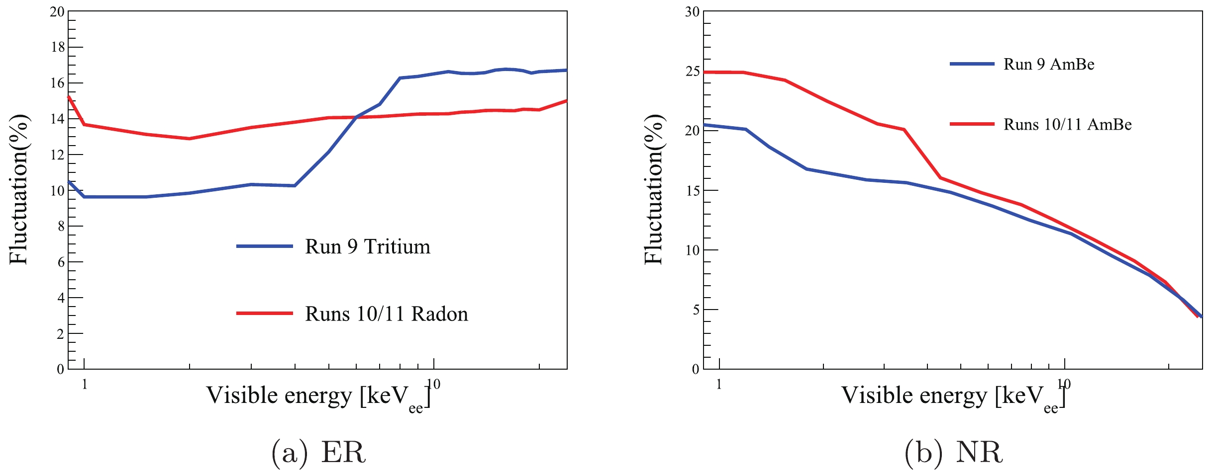
Figure 4. (color online) The empirical fluctuation parameter f as a function of visible energy for the ER (left) and NR (right) data, both in electron equivalent energy keVee
-
The detector model is used to convert
$ n_{\rm{ph}} $ and$ n_{\rm{e}} $ to detected S1 and S2. For the R11410-20 PMTs used in PandaX-II, the double-photoelectron emission probability by the 178 nm scintillation photons$ p_{\rm{2pe}} $ is recorded as$ 0.21\pm0.02 $ from the data [6]. Therefore, the total detected photons ($ N_{\rm{dph}} $ ) is given by$ {N_{\rm{dph}}} = {\rm{Binom}}(n_{\rm{ph}}, {{\rm{PDE}}}/(1 + {p_{\rm{2pe}}})), $

(4) in which
$ {\rm{Binom}}(N,p) $ refers to a binomial distribution with N throws and a probability p, and$ {\rm{PDE}}/(1+p_{\rm{2pe}}) $ is the binomial probability to detect a photon.$ N_{\rm{dph}} $ is randomly distributed onto the two arrays of PMTs (55 each) according to the measured top/bottom ratio from the data ($ \sim $ 1:2), to yield a significantly accurate simulation of the total PMT hits. Each detected photons is then fluctuated by$ p_{\rm{2pe}} $ , leading to the total photoelectrons$ {N_{\rm{PE}}} = {N_{\rm{dph}}} + {\rm{Binom}}({N_{\rm{dph}}}, p_{\rm{2pe}})\,. $

(5) S1 can be subsequently obtained by applying the single photoelectron (SPE) resolution, modeled as a Gaussian with a
$ \sigma_{\rm{SPE}} $ of 33% [16]$ S1 = {{\rm{Gaus}}(N_{\rm{PE}}},\sigma_{\rm{SPE}} \times \sqrt{N_{\rm{PE}}})\,. $

(6) Each S1 is required to have at least three hits, with each hit larger than 0.5 PE to simulate the single channel readout threshold and the multiplicity cut in the analysis [6].
Similarly, S2 is simulated based on
$ n_{\rm{e}} $ using detector parameters from the data. For each event, the drift time$ t_{\rm{drift}} $ is randomized according to the data distribution, leading to an electron survival probability$s = $ $ \exp(-t_{\rm{drift}}/\tau)$ with the electron lifetime τ obtained from the data. At the liquid level, the total electrons is$ {N_{\rm{e}}^{'}} = {\rm{Binom}}(n_{\rm{e}}, s)\,. $

(7) The total extracted electrons
$ N_{\rm{e}}^{''} $ and S2 can be simulated as$ \begin{aligned}[b] N_{\rm{e}}^{''} =& {\rm{Binom}}(N_{\rm{e}}^{'}, {\rm{EEE}})\, ,\\ S2 =& {\rm{Gaus}}({N_{\rm{e}}^{''}} \times {\rm{SEG}},\sigma_{\rm{SE}} \times \sqrt{{N_{\rm{e}}^{''}}})\,, \end{aligned} $

(8) where
$ \sigma_{\rm{SE}}\sim 8.3 $ PE is the Gaussian width for the single electron signals.As discussed in Ref. [6], the nonlinearities in S1 and S2 owing to baseline suppression firmware are measured from the data, denoted by
$ f_1(S1) $ and$ f_2(S2) $ . So the detected S1 and S2 are$ S1_{d} = S1 \times f_{1}\,, S2_d = S2 \times f_{2}\,. $

(9) Finally, the data selection efficiency is parameterized as a Fermi-Dirac function
$ \epsilon(S1_d) = \frac{1}{1+\exp\left(\dfrac{S1_d-p_0}{p_1}\right)}\,, $

(10) where
$ p_0 $ and$ p_1 $ are determined by fitting to calibration data. We observed that the S2 efficiency can be omitted, presumably owing to the large$ S2_{\rm{raw}} >100$ PE selection cut that is signficantly above the trigger threshold of 50 PE [17]. The final efficiency at high energy end is absorbed in this analysis by normalizing the data with the simulation. -
In this section, the ER and NR response models will be fitted against the calibration data in S1 and S2 using unbinned likelihood. The systematic uncertainties of the models are quantified by a likelihood ratio approach.
-
As an initial approximation,
$ L_y $ can be fitted from the medians of the calibration data distribution by$ L_y^0(E_{\rm{rec}}/L) = \frac{S1}{{{\rm{PDE}}}\times E_{\rm{rec}}/L}\,, $

(11) where
$ E_{\rm{rec}} $ (Eq. (1)) is the reconstructed energy including all detector effects, and the$\dfrac{{E_{\rm rec}}}{L}$ is the estimate of$ E_0 $ . The true$ L_y $ can be parameterized as$ L_y(E_0) = L_y^0(E_0) + \sum\limits_{n = 0} ^{4} c_n P_n(E_0) \,, $

(12) in which
$ P_n(E_0) $ is the nth order Legendre polynomial functions, and$ c_n $ can be fitted to data.For a given model, a two-dimensional probability density function (PDF) in (S1,S2) is produced with a large statistics simulation described in Secs. IVA and IVB using the following sets of parameters: a) PDE, EEE and SEG constrained by their Gaussian priors (Table 1), with the anti-correlation between PDE and EEE embedded (see Ref. [18]), b) parameters for
$ \epsilon(S1_d) $ in Eq. (10), with a flat sampling of$ p_0\in(2,5) $ and$ p_1\in(0,1) $ , respectively, and c) a 4th order Legendre polynomial expansion for$ L_y $ in Eq. (12), with$ c_n $ ($ n = 0,1,2,3,4 $ ) uniformly sampled from -5 to 5. Experiments were performed to investigate if the polynomial expansion converges after the 3rd power. Parameters such as the fluctuation in the electron lifetime and, that are independently determined from the data were fixed in the simulation. For the baseline suppression nonlinearities, the smooth probability distributions determined from the data in Ref. [6] are sampled.To compare the data to the PDF, a standard unbinned log likelihood function is defined in the space of (S1,S2) as
$ -2\ln{\cal{L}} = \sum\limits_{i = 1}^{N} -2\ln(P(S1^i, S2^i))\,, $

(13) where
$ P(S1^i, S2^i) $ is the probability density for a given calibration data point i, and N is the total number of events for each calibration data set. -
An independent parameter scan is performed to determine the best fit model for each calibration data set. The best fit corresponds to the PDF that yields the minimum
$ -2\ln{\cal{L}} $ . For illustration, the centroids and 90% quantiles of the best fit models from the four data sets are shown in Fig. 3, where the data are consistent.The parameter space allowable by the calibration data is determined based on the likelihood ratio approach in Ref. [19]. For each set of fixed parameters, 1000 mock data runs are produced with equal although Poisson fluctuated statistics as the calibration data. The test statistic for each mock run is defined as the difference between the log likelihood calculated using the fixed point PDF, and the global minimum value from the parameter scan as,
$ \Delta {\cal{L}} = -2{\ln} {\cal{L}}_{\rm{fixed}} - (-2{\ln}{\cal{L}}_{\rm{min}})\,. $

(14) The distributions of
$ \Delta {\cal{L}} $ for the mock data generated from the best fit parameters for the four calibration data sets are shown in Fig. 5. The blue dashed regions refer to the 90% integrals from zero, beyond which the difference between the mock data set and its own PDF is less likely. The 90% boundary values for$ \Delta {\cal{L}} $ at other parameter space points are similar. Therefore,$ \Delta {\cal{L}} $ of the real data is tested around the best fit, and the allowable space is defined by the 90% boundaries in Fig. 5. The corresponding allowable range of distributions in recoil energy, S1, and S2 are shown in Fig. 6, together with the calibration data that were consistent.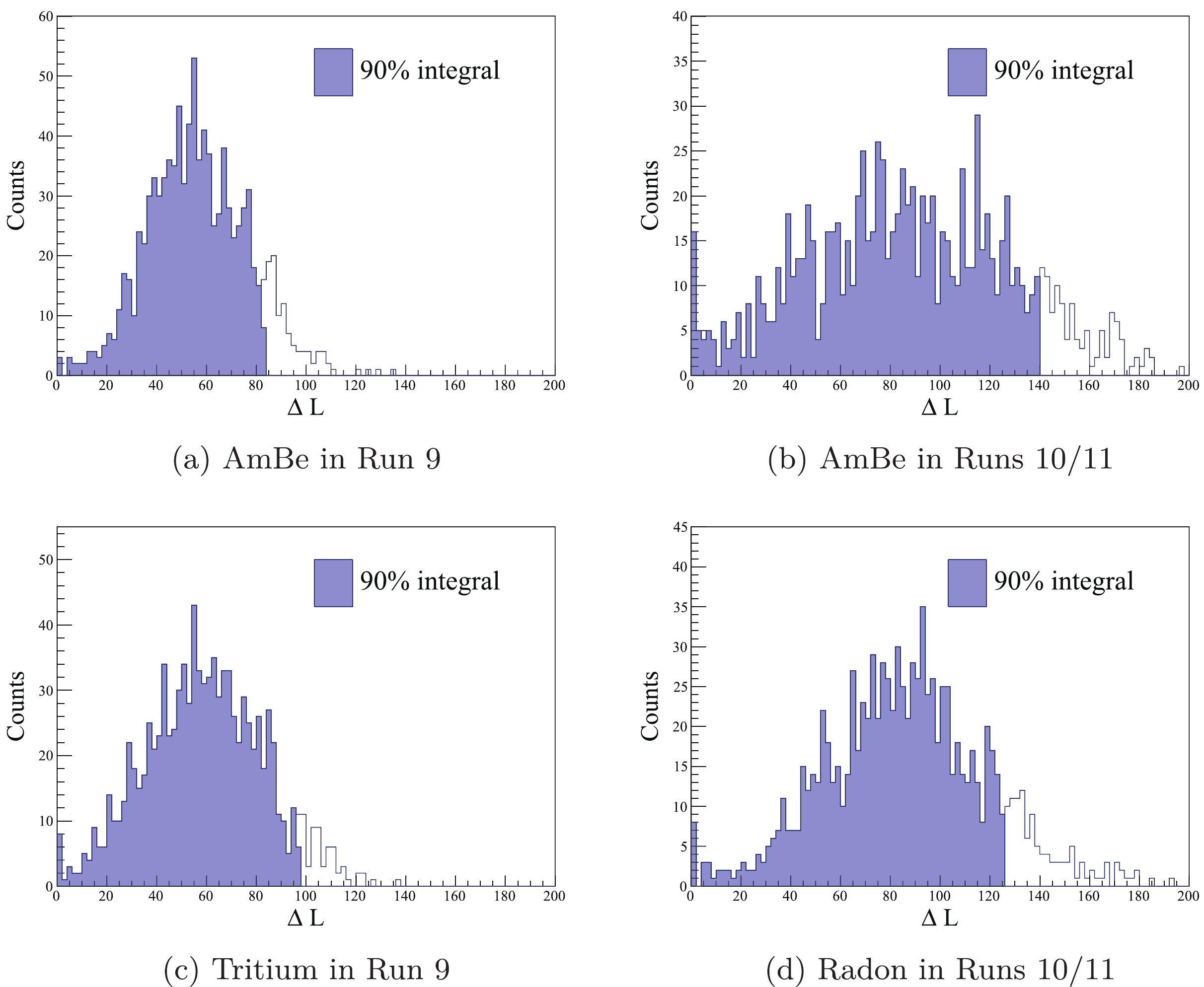
Figure 5. (color online) The distribution of
$ \Delta {\cal{L}}$ for mock calibration data sets generated at the best fit parameter points. The shaded regions indicate the 90% integrals.
Figure 6. (color online) The comparison of calibration data (points) and model (shaded bands = 90% allowable) in the recoil energy, S1, and S2, in Run 9 and Runs 10/11. For the 220Rn energy distribution (j), the decrease at high energy end is due to the 150 PE S1 range cut.
The resulting best fit
$ Q_y $ and$ L_y $ for the NR and ER events are shown in Fig. 7, overlaid with the world data, and the native NEST2.0 predictions [4]. The shaded bands indicate the 90% allowable model space, with uncertainties owing to detector parameters and statistics of the calibration data naturally incorporated. Our NR models cover a wide energy range from 4 to 80 keVnr. At the two drift fields (400 and 317 V/cm), our optimal NR models are consistent as expected. For the$ Q_y $ distribution with recoil energy from 4 to 15 keVnr, there is significant spread among the world data, wherein our$ Q_y $ is significantly consistent with Ref. [20] (Xenon-1T 2019), although lower than others. The NEST2.0 global fit, predominantly driven by data from Ref. [21] (LUX DD), has a higher$ Q_y $ than that of our model. The global data consistency improved significantly above 15 keVnr.$ L_y $ of our NR models, in contrast, is consistent with most world data, except some insignificant tension at above 25 keVnr with Ref. [22] (Manzur 2010), which bears large uncertainties by itself.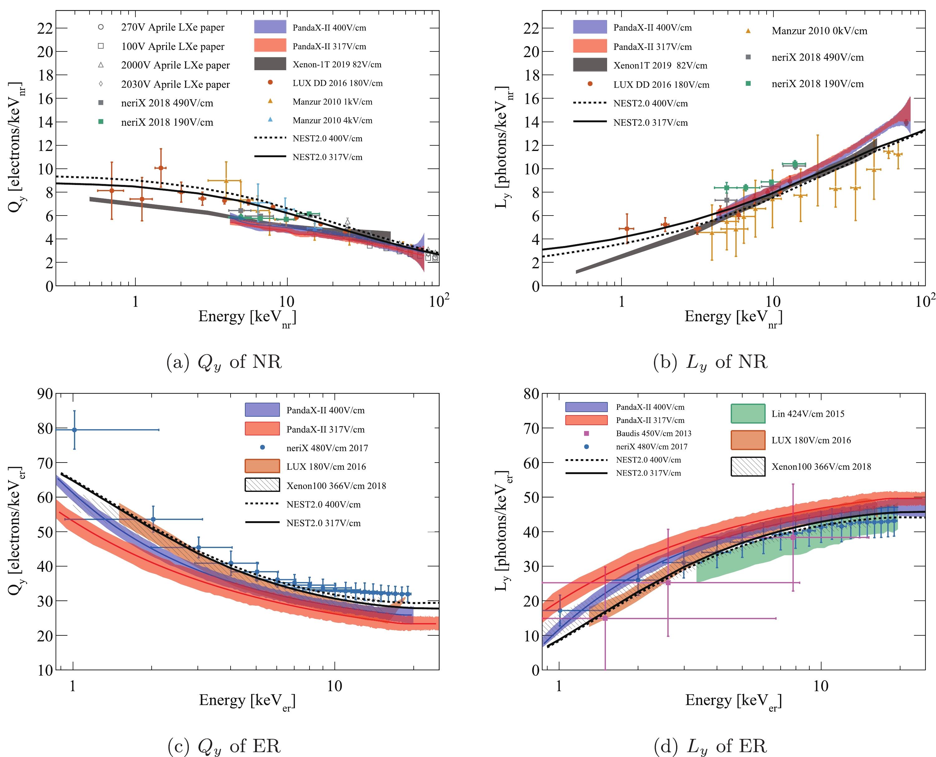
Figure 7. (color online) Charge yield
$ Q_y$ (a) and light yield$ L_y$ (b) of the NR and$ Q_y$ (c) and$ L_y$ (d) of the ER obtained from the PandaX-II data: blue=400 V/cm, red=317 V/cm. Overlaid world data include: NR from Refs. [21, 22, 26-29], and ER from Refs. [7, 24, 25, 30], as indicated in the legend. The native NEST2.0 predictions are drawn in black curves, solid (317 V/cm), and dashed (400 V/cm). The XENON1T responses [20] are not included in the ER figures since the operation field (81 V/cm) is significantly different from the PandaX-II conditions, and for visual clarity.For the ER models,
$ Q_y $ ($ L_y $ ) for Run 9 is higher (lower) than that for Runs 10/11. This behavior is expected because the initial ionized electrons are less likely to be recombined in stronger drift field. Our model at 400 V/cm is consistent with Ref. [23] (Xenon100) at similar drift field, although there is some considerably insconsistency with Refs. [24, 25] (neriX 480 V/cm, Lin 424 V/cm). Our$ Q_y $ ($ L_y $ ) at 317 V/cm is lower (higher) than the world data, including that from Ref. [21] (LUX) taken at 180 V/cm (and that from Ref. [20] at 81 V/cm, not drawn), and the native NEST2.0 predictions. The key systematic effects can cause the differences in our data interpretation. For example, the three-dimensional uniformity correction for S1 and S2, correlated with position reconstruction, can lead to uncertainties in the PDE and EEE. At high energy, the saturation of PMTs and the afterpulsing under large S2s are also potential source of biases in these parameters. At low energy, the uncertainty of the selection efficiency, the BLS nonlinearity, and uncertainties in recoil energy distributions (particularly for NR events) can lead to systematics in the low energy response curves. Because most systematics can affect global measurements, investigations on systematics are desirable.Notwithstanding the global comparison, for PandaX-II, models determined from in situ calibrations are the most self-consistent models to be used in the PandaX-II dark matter search data. Our best fit models presented herein have been adopted in the analysis in Ref. [6], with an overall uncertainty of 20% in the dark matter rate normalization to record global uncertainties.
-
We present an ER and NR responses from a PandaX-II detector based on calibration data from operation at two different drift fields (400 and 317 V/cm). The empirical best fits to the data and model uncertainties are obtained, indicating significant consistency between the data and our models. In comparison to those presented in Refs. [18, 31], the models in this work cover the entire PandaX-II data taking period, with a signficantly extended energy ranges from 4 to 80 keVnr(NR) and 1 to 25 keV
$ _{\rm{ee}} $ (ER). At the two drift fields, our NR models are consistent, and our ER models exhibit a relative shift. Both behaviors are consistent with expectation.Our models are also compared to some world data. Our NR models lie in the large global spread. For the ER response, our model yields a higher (lower)
$ L_y $ ($ Q_y $ ) in comparison to most world data, indicating some unaccounted systematic uncertainties in our or other measurements. These discrepancies encourage continuous calibration effort and further investigations of systematics in the data. Finally, the analysis approach presented herein is generalized and can be applied to similar noble liquid TPC experiments. -
We thank supports from Double First Class Plan of the Shanghai Jiao Tong University for their support. We also thank the Chinese Academy of Sciences Center for Excellence in Particle Physics (CCEPP) for thei sponsorship, We are grateful to the Hongwen Foundation in Hong Kong, and Tencent Foundation in China. Finally, we thank the CJPL administration and the Yalong River Hydropower Development Company Ltd. for indispensable logistical and other support.
Determination of responses of liquid xenon to low energy electron and nuclear recoils using a PandaX-II detector
- Received Date: 2021-02-07
- Available Online: 2021-07-15
Abstract: We present a systematic determination of the responses of PandaX-II, a dual phase xenon time projection chamber detector, to low energy recoils. The electron recoil (ER) and nuclear recoil (NR) responses are calibrated, respectively, with injected tritiated methane or 220Rn source, and with 241Am-Be neutron source, in an energy range from 1-25 keV (ER) and 4-80 keV (NR), under the two drift fields, 400 and 317 V/cm. An empirical model is used to fit the light yield and charge yield for both types of recoils. The best fit models can describe the calibration data significantly. The systematic uncertainties of the fitted models are obtained via statistical comparison to the data.


 DownLoad: