


 Abstract
 HTML
HTML Reference
 Related
 PDF
PDF


-
The existence of dark matter (DM) is supported by various astronomical observations at different scales, but the nature of DM particles is still unknown. As an important probe in indirect DM detection, the antiparticles in cosmic rays (CR) may shed light on the properties of DM. In recent years, a number of experiments have shown an unexpected structure in the CR positron data [1-4], which could be related to DM annihilation or decay [5-8]. Unlike CR positrons, the CR antiproton flux data from PAMELA [9], BESS-polar II [10] and AMS-02 [11] do not show significant discrepancies with the secondary production of antiprotons, and these null results can be used to place stringent constraints on the DM annihilation cross-sections [12-15].
CR heavy anti-nuclei such as antideuterium (
$ \overline{\text{D}} $ ) and antihelium-3 ($ ^3\overline{\text{He}} $ ) are postulated to be important probes for DM [16-18]. The$ \overline{\text{D}} $ and$ ^3\overline{\text{He}} $ in CR can be generated as secondary productions by collisions between primary CR particles and interstellar gas, or they can be produced by DM annihilation or decay. However, the secondary$ \overline{\text{D}} $ and$ ^3\overline{\text{He}} $ are boosted to high kinetic energies because of the high production threshold in$ pp $ -collisions (17$ m_{p} $ for$ \overline{ \rm{D}} $ and 31$ m_{p} $ for$ ^{3}\overline{\text{He}} $ , where$ m_{p} $ is the proton mass), and thus the signal from DM can be distinguished in low energy regions (below GeV per nucleon). Although the fluxes of anti-nuclei decrease rapidly with the increase of the atomic mass number A, the high signal-to-background ratio at low energies and experiments with high sensitivities (such as AMS-02 [19, 20] and GAPS [21]) make it possible to distinguish the contributions from DM interactions. Furthermore, an advantage for considering$ \overline{\text{D}} $ and$ ^3\overline{\text{He}} $ is that their productions are highly correlated with CR antiprotons, so the uncertainties of the$ \overline{\text{D}} $ and$ ^3\overline{\text{He}} $ fluxes can be greatly reduced by the CR$ \bar{p} $ data [22].In the literature (for a recent review, see Ref. [23]), the analysis of the DM-produced
$ \overline{\text{D}} $ and$ ^3\overline{\text{He}} $ are focused on the low kinetic energy regions, which we refer to as the low energy window. In our previous analysis [22], we studied the prospects of detecting DM through low energy antihelium. We systematically analysed the uncertainties from propagation models, DM density profiles and MC generators, and reduced the uncertainties by constraining the DM annihilation cross-sections with the AMS-02$ \bar{p}/p $ data. However, the low energy window suffers from the uncertainties of solar activity (solar modulations). In this work, we investigate the possibility of probing DM with high energy CR$ \overline{\text{D}} $ and$ ^3\overline{\text{He}} $ particles. In high energy regions (typically above 100 GeV per nucleon), the flux of primary CR particles drops quickly (the flux of CR proton is proportional to$ E^{-2.75} $ ), which leads to a suppression of the high energy secondary CR particles. As a result, the fluxes of anti-nuclei produced by DM annihilation may exceed the secondary background and open a high energy window for probing DM.We use the Monte Carlo (MC) event generators PYTHIA 8.2 [24, 25], EPOS-LHC [26, 27] and DPMJET-III [28] to fit the coalescence momenta for anti-nuclei with experiments including ALEPH [29], CERN ISR [30] and ALICE [31], and generate the energy spectra of anti-nuclei. The propagation of CR particles is calculated using the GALPROP code. We use the AMS-02 [11] and HAWC
$ \bar{p}/p $ data [32] and the HESS galactic center (GC)$ \gamma $ -ray data [33, 34] to constrain the DM annihilation cross-sections. We find that the conclusion depends on the choice of DM density profiles. For a large DM mass ($ \gtrsim 10 $ TeV) with the relatively flat “Cored” type DM profile, the high energy window exists, while for a typical steep DM profile like the “Cuspy” type, the high energy window closes.This paper is organized as follows. In Section II, we briefly review the coalescence model and determine the coalescence momenta for anti-nuclei by fitting the ALEPH, ALICE and CERN-ISR data. In Section III, we review the theory of CR propagation. In Section IV, we constrain the DM annihilation cross-section by using the
$ \bar{p}/p $ data from AMS-02 and HAWC and$ \gamma $ -ray data from HESS. The fluxes of$ \overline{\text{D}} $ and$ ^3\overline{\text{He}} $ for direct DM annihilation and annihilation through mediator channels are presented in Section V. The conclusions are summarized in Section VI. -
The formation of anti-nuclei can be described by the coalescence model [35-37], which uses a single parameter, the coalescence momentum
$ p_0^{ \bar{{A}}} $ , to quantify the probability of anti-nucleons merging into an anti-nucleus$ \bar{{A}} $ . The basic idea of this model is that anti-nucleons combine into an anti-nucleus if the relative four-momenta of a proper set of nucleons is less than the coalescence momentum. For example, the coalescence criterion for$ \overline{\text{D}} $ is written as:$ ||k_{\bar{p}}-k_{\bar{n}}|| = \sqrt{(\Delta \vec{k})^2-(\Delta E)^2} < p_0^{ \overline{\mathrm{D}}}, $

(1) where
$ k_{\bar{p}} $ and$ k_{\bar{n}} $ are the four-momenta of the antiproton and antineutron respectively, and$ p_0^{\bar{ \mathrm{D}}} $ is the coalescence momentum of$ \overline{\text{D}} $ . If we assume that the momentum distributions of the$ \bar{p} $ and$ \bar{n} $ in one collision event are uncorrelated and isotropic, the spectrum of$ \overline{\text{D}} $ can be derived by the phase-space analysis:$ \gamma_{\bar{ \mathrm{D}}} \frac{{\rm d}^{3}N_{\bar{ \mathrm{D}}}}{{\rm d}^{3}\vec{k}_{\bar{ \mathrm{D}}}} (\vec{k}_{\bar{ \mathrm{D}}}) = \frac{\pi}{6} \left(p_{0}^{\bar{ \mathrm{D}}}\right)^{3} \cdot \gamma_{\bar p} \frac{{\rm d}^{3}N_{\bar p}}{{\rm d}^{3}\vec{k}_{\bar p}}(\vec{k}_{\bar p}) \cdot \gamma_{\bar n} \frac{{\rm d}^{3}N_{\bar n}}{{\rm d}^{3}\vec{k}_{\bar n}}(\vec{k}_{\bar n}) , $

(2) where
$ \gamma_{\bar{ \mathrm{D}}, \bar p, \bar n} $ are the Lorentz factors, and$ \vec{k}_{\bar p}\approx \vec{k}_{\bar n}\approx \vec{k}_{\bar{ \mathrm{D}}}/2 $ .For
$ ^3\overline{\text{He}} $ , we adopt the same coalescence criterion as in our previous analysis [22]. We compose a triangle using the norms of the three relative four-momenta$ l_1 = ||k_1-k_2||,\; \; l_2 = ||k_2-k_3|| $ and$ l_3 = ||k_1-k_3|| $ , where$ k_1, k_2, k_3 $ are the four-momenta of the three anti-nucleons respectively. Then, making a circle with minimal diameter to envelop the triangle, if the diameter of this circle is smaller than$ p_0^{ \overline{\mathrm{He}}} $ , an$ ^3\overline{\text{He}} $ is generated. If the triangle is acute, the minimal circle is just the circumcircle of this triangle, and the coalescence criterion can be expressed as follows:$ d_{\mathrm{circ}} \!=\! \frac{l_1l_2l_3}{\sqrt{(l_1\!+\!l_2\!+\!l_3)(-l_1\!+\!l_2\!+\!l_3)(l_1\!-\!l_2\!+\!l_3)(l_1\!+\!l_2\!-\!l_3)}}< p_0^{ \overline{\mathrm{He}}}. $

(3) Otherwise, the minimal diameter is equal to the longest side of the triangle, and the criterion can be simply written as
$ \text{max}\{l_1,l_2,l_3\} < p_0^{ \overline{\mathrm{He}}} $ . See Ref. [22] for more details.We use the MC generators PYTHIA 8.2, EPOS-LHC and DPMJET-III to simulate the hadronization after the DM annihilations and
$ pp- $ collisions, then use the coalescence model to produce anti-nuclei from the final state$ \bar{p} $ or$ \bar{n} $ . The spatial distance between each pair of anti-nucleons also needs to be considered, because the anti-nucleons should be close enough to undergo nuclear reactions then merge into anti-nuclei. We set all the particles with lifetime$ \tau \gtrsim 2\,\, \mathrm{fm}/c $ to be stable, to ensure that every pair of anti-nucleons is located within a short enough distance [17], where 2 fm is approximately the size of the$ ^3\overline{ \rm{He}} $ nucleus.The values of the coalescence momenta should be determined by the experimental data, which are often released in the form of coalescence parameters
$ B_A $ . The definition of the coalescence parameter$ B_A $ is expressed by the formula:$ E_A\frac{{\rm d}^3N_A}{{\rm d}p_A^3} = B_A \left(E_p\frac{{\rm d}^3N_p}{{\rm d}p_p^3}\right)^Z \left(E_n\frac{{\rm d}^3N_n}{{\rm d}p_n^3}\right)^N , \ \ \ \vec{p}_p = \vec{p}_n = \vec{p}_A/A ,$

(4) where
$ A = Z+N $ is the mass number of the nucleus, and Z and N are the proton number and the neutron number respectively. Under the assumption that the momentum distributions of the$ \bar{p} $ and$ \bar{n} $ are uncorrelated and isotropic, the relation$ B_A\propto p_0^{3(A-1)} $ is expected by comparing Eq. (2) and Eq. (4). However, the jet structure and the correlation between$ \bar{p} $ and$ \bar{n} $ play important roles in the formation of anti-nuclei. So we derive the coalescence momenta by using the MC generators to fit the experimental data, and thus the effect of jet structures and correlations are included.To derive the coalescence momentum of
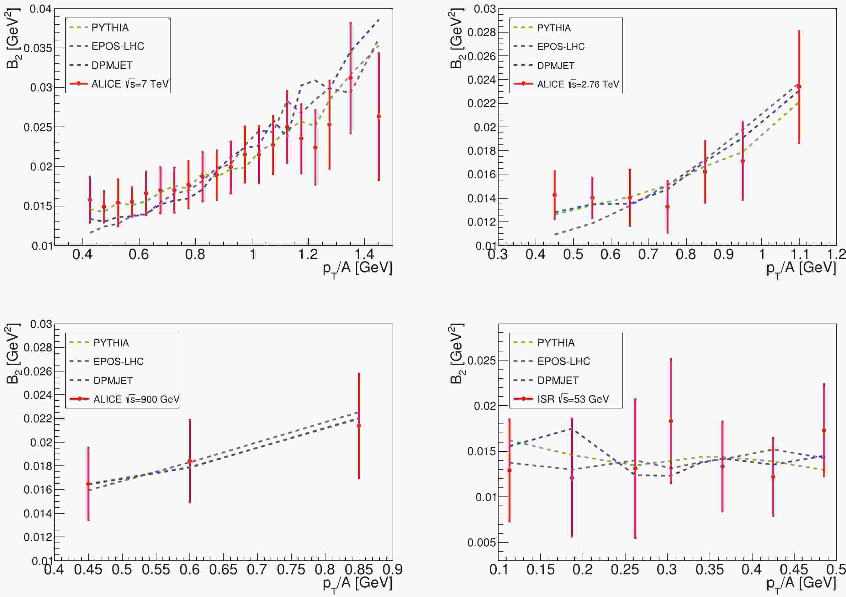
$ \overline{\mathrm{D}} $ in$ pp $ collisions, we follow the procedures described in Ref. [22] to fit the coalescence parameter$ B_2 $ data from the ALICE-7 TeV, 2.76 TeV, 900 GeV [31] and ISR-53 GeV [30] experiments. We use MC generators to simulate these experiments, and record the momenta information of$ \bar{p} $ ,$ \bar{n} $ that are possible to form a$ \overline{\mathrm{D}} $ . We select the$ \bar{p} $ and$ \bar{n} $ according to a sufficiently large coalescence momentum$ p_{0,\text{max}} $ (600 MeV for$ \overline{\mathrm{D}} $ , 1 GeV for$ \overline{\mathrm{He}} $ ), and then calculate the spectra of$ \overline{\text{D}} $ for different$ p_0^{ \overline{\mathrm{D}}} $ values that are smaller than$ p_{0,\text{max}} $ . The$ B_2 $ values are calculated by using Eq. (4), and we perform a$ \chi^2 $ analysis to find the value of$ p_0^{ \overline{\mathrm{D}}} $ . The best-fit$ B_2 $ values are shown in Fig. 1. We find$ \chi^2_{\text{min}}/{d.o.f}< 1 $ for all these fits, which means the fitting results are in good agreement with the experimental data. As shown by the figure, the$ p_T $ -dependences are reproduced well by the coalescence model and the MC generators.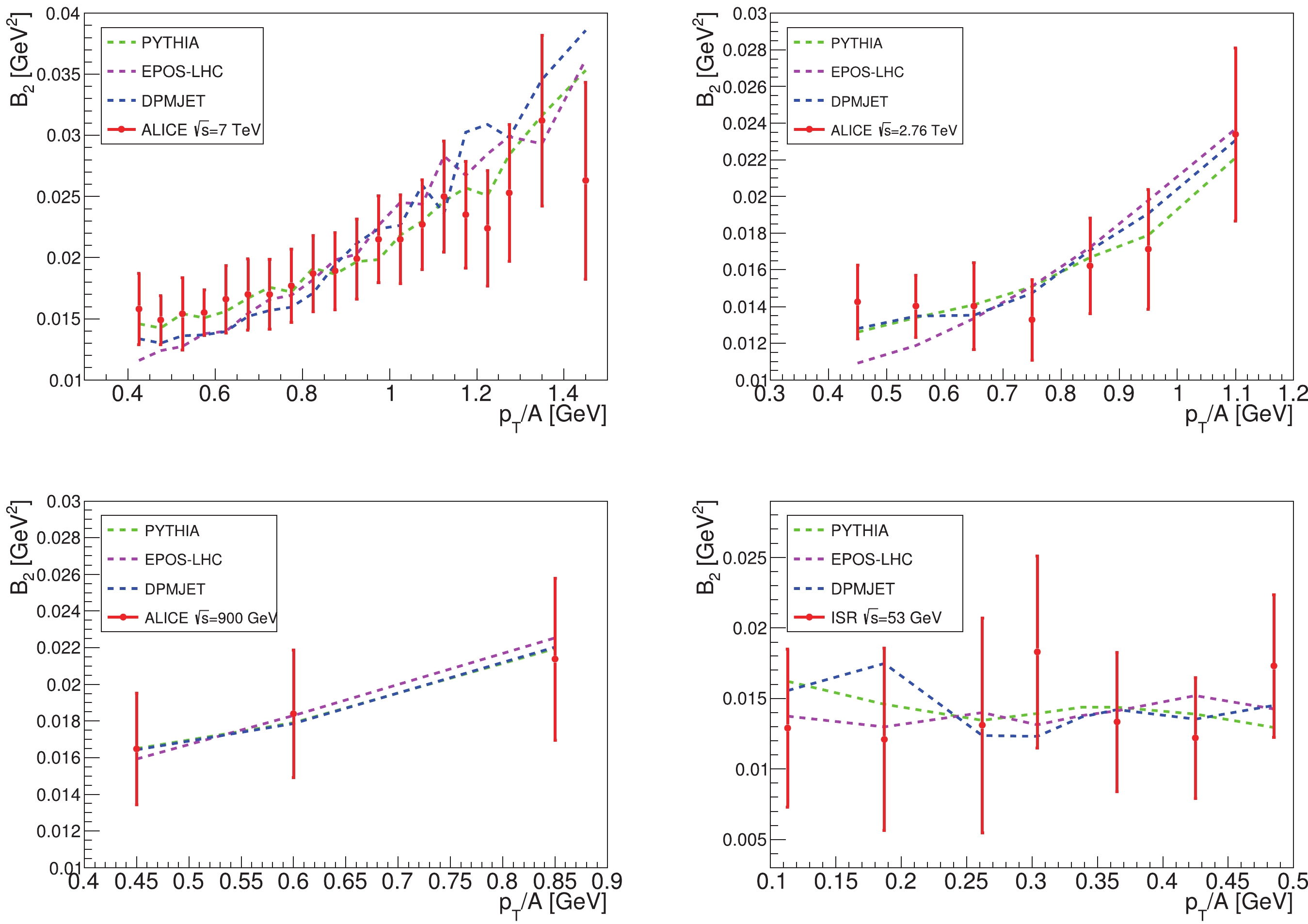
The fitting results for
$ p_0^{ \overline{\mathrm{D}}} $ are listed in Table 1. The values in parentheses are the results given by the ALICE group, which are only available for the ALICE 7 TeV and ISR-53 GeV experiments with the PYTHIA 8.2 and EPOS-LHC generators. We can see that for ALICE 7 TeV, our best-fit values are in good agreement with those from the ALICE group, but for ISR-53 GeV, our results are larger. This is partly because the ALICE group has only generated the energy spectra of$ \overline{\text{D}} $ for six$ p_0^{ \overline{\mathrm{D}}} $ values [31], and used the isotropic approximation$ B_A\approx p_0^{3(A-1)} $ to interpolate the spectra for other$ p_0^{ \overline{\mathrm{D}}} $ values, while we generate the$ \overline{\text{D}} $ spectra for every integer number MeV and do not need the approximation. Moreover, in fitting the ISR-53 GeV experiment, the ALICE group has manually rescaled the spectra of$ \bar{p} $ generated by MC to better reproduce the experimental data, while for self-consistency we do not make this correction.MC generators ALICE 7/TeV ALICE 2.76/TeV ALICE 900/GeV ISR 53/GeV PYTHIA 8.2 $214^{+2}_{-3}~(216\pm 8)$ 

$206^{+4}_{-4}$ 

$231^{+9}_{-9}$ 

$233^{+10}_{-13}~(188\pm8)$ 

EPOS-LHC $210^{+2}_{-3}~(200\pm10)$ 

$208^{+6}_{-3}$ 

$235^{+8}_{-9}$ 

$211^{+7}_{-11}~(190\pm8)$ 

DPMJET-III $201^{+1}_{-3}$ 

$197^{+4}_{-4}$ 

$219^{+8}_{-8}$ 

$195^{+9}_{-12}$ 

Table 1. Best-fit values of
$ p_0^{\overline{\mathrm{D}}} $ in units of MeV, derived by fitting the$ pp $ -collision data with three MC generators, PYTHIA 8.2 [24, 25], EPOS-LHC [26, 27], and DPMJET-III [28]. The$ p_0^{\overline{\mathrm{D}}} $ values do not show a clear relation with the$ \sqrt{s} $ value of the experiments. The values in parentheses are fitting results given by the ALICE group.In Fig. 2, we show the
$ p_0^{ \overline{\mathrm{D}}} $ values for different$ pp $ collision experiments with various MC generators. As can be seen,$ p_0^{ \overline{\mathrm{D}}} $ does not show a clear relation with the$ \sqrt{s} $ values of the experiments. Since the fitting results for different center-of-mass energies are similar, we assume that the$ p_0^{\overline{\mathrm{D}}} $ value does not vary with the$ \sqrt{s} $ of the experiment. By fitting these$ p_0^{\overline{\mathrm{D}}} $ , we get$ p_0^{\overline{\mathrm{D}}}(\texttt{PYTHIA)} = 213\pm2 $ MeV,$ p_0^{\overline{\mathrm{D}}}(\texttt{EPOS-LHC)} = 211\pm $ $ 2 $ MeV, and$ p_0^{\overline{\mathrm{D}}}(\texttt{DPMJET)} = $ $ 201\pm2 $ MeV for$ pp $ collisions.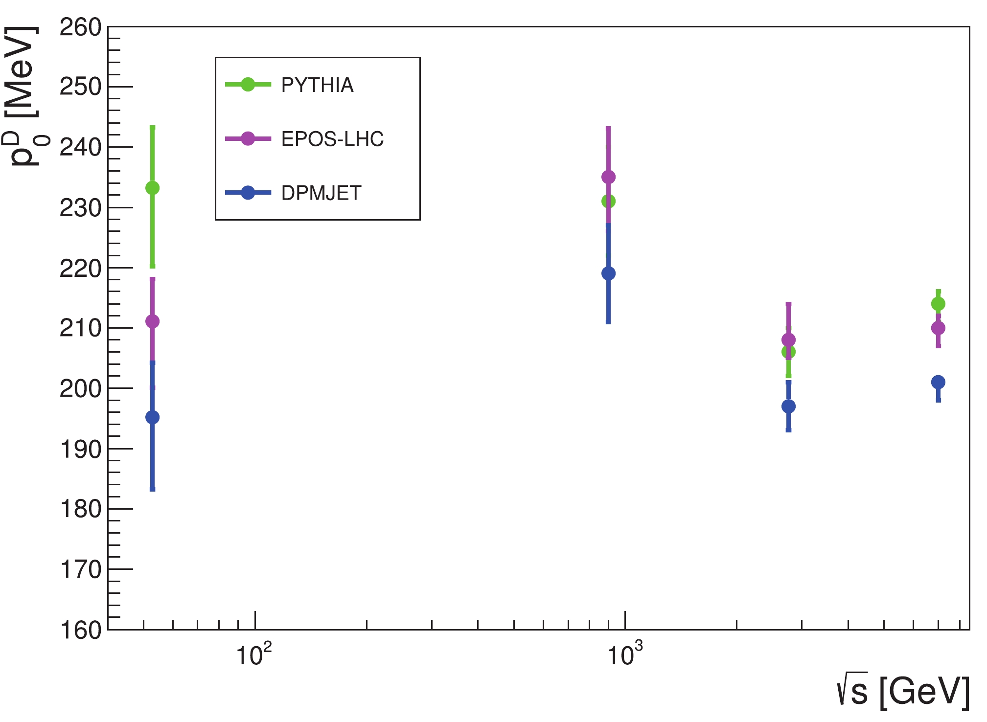
Figure 2. (color online)
$ p_0 $ values of$ {\overline{\mathrm{D}}} $ from fitting the$ pp $ collision data with three MC generators.By using PYTHIA to fit the
$ B_2 = 3.3\pm1.0\pm0.8\times10^{-3} $ data from the ALEPH$ e^+e^-\rightarrow Z^0 \rightarrow \overline{\mathrm{D}} $ experiment [29], we find$ p_0^{\overline{\mathrm{D}}}(Z^0) = 190^{+23}_{-27} $ MeV. Considering the similarity between the dynamics of the$ Z^0 $ decay and DM annihilation, we set$ p_0^{\overline{\mathrm{D}}}(Z^0) $ to be the coalescence momentum for the DM annihilation process$ \chi\chi \rightarrow \overline{\mathrm{D}} + X $ .For
$ ^3\overline{\text{He}} $ , we adopt the$ p_0^{\overline{\mathrm{He}}} $ value obtained in our previous work [22], which determining$ p_0^{\overline{\mathrm{He}}} $ by fitting the ALICE$ \sqrt{s} = 7 $ TeV$ pp $ -collision data. The results are listed in Table 2. Note that$ ^3\overline{\text{He}} $ particles can be produced from two channels: direct formation from the coalescence of$ \bar{p}\bar{p}\bar{n} $ , or through the$ \beta $ -decay of an antitriton$ \overline{\text{T}} $ ($ \bar{p}\bar{n}\bar{n} $ ). The direct formation channel is suppressed by the Coulomb repulsion between the two antiprotons, so some previous works only considered the antitriton channel. However, our calculation shows that the direct formation channel is not negligible. The coalescence momentum of$ ^3\overline{\mathrm{He}} $ is only slightly smaller than that of$ \overline{\text{T}} $ , and the Gamow factor$ \mathcal{G}\sim \exp(-2\pi\alpha m_p/p_0^{\overline{\mathrm{He}}}) \approx 0.8 $ [38], which indicates that the Coulomb repulsion may not be significant. From these facts, it is reasonable to ignore the Coulomb repulsion in the MC simulation, and the contributions from both channels are included in this work. Our MC calculation shows that about 30% of$ ^3\overline{\mathrm{He}} $ is produced through the direct formation channel. Due to the lack of$ e^+e^-\rightarrow ^3\overline{\text{He}} $ experiment data, we set$ p_0^{\overline{\mathrm{He}}/\overline{\mathrm{T}}}(\texttt{PYTHIA)} $ to be the coalescence momentum for the DM annihilation process$ \chi\chi \rightarrow \overline{\mathrm{He}}/\overline{\mathrm{T}} + X $ . It is known that the coalescence momentum varies for different processes and center-of-mass energies [39], and the relation$ B_A\approx p_0^{3(A-1)} $ makes$ p_0 $ a crucial factor for the uncertainties of the final fluxes. In some previous analyses, the value of$ p_0^{\overline{\mathrm{He}}} $ was estimated using various approaches, for example by using the binding energy relation between$ p_0^{\overline{\mathrm{He}}} $ and$ p_0^{\overline{\mathrm{D}}} $ , or assuming the ratio$ p_0^{\overline{\mathrm{He}}}/p_0^{\overline{\mathrm{D}}} = p_0^{\mathrm{He}}/p_0^{\mathrm{D}} $ [17], and some works just set$ p_0^{\overline{\mathrm{He}}} = p_0^{\overline{\mathrm{D}}} $ [18]. The$ p_0^{\overline{\mathrm{He}}} $ results from these approaches are different. It is worth mentioning that our$ p_0^{\overline{\mathrm{He}}} $ value is relatively small compared to previous works, which leads to conservative DM contributions.MC generator PYTHIA 8.2 EPOS-LHC DPMJET-III $p_0^{\overline{\mathrm{He}}}$ /MeV

$224^{+12}_{-16}$ 

$227^{+11}_{-16}$ 

$212^{+10}_{-13}$ 

$p_0^{\bar{\mathrm{T}}}$ /MeV

$234^{+17}_{-29}$ 

$245^{+17}_{-30}$ 

$222^{+16}_{-26}$ 

Table 2. Best-fit values of
$ p_0^{\overline{\mathrm{He}}} $ and$ p_0^{\bar{\mathrm{T}}} $ from Ref. [22], obtained by fitting the ALICE$ pp $ -collision data at$ \sqrt{s} = 7 $ TeV for three MC generators, PYTHIA 8.2, EPOS-LHC, and DPMJET-III.For the primary anti-particles originating from DM annihilations, the injection spectra are calculated using PYTHIA 8.2. We simulate the annihilation of Majorana DM particles by a positron-electron annihilation process
$ e^+e^- \rightarrow \phi^* \rightarrow f\bar{f} $ , where$ \phi^* $ is a fictitious scaler singlet and f is a standard model final state. We set$ \sqrt{s} = 2m_{\chi} $ and switch off all initial-state-radiations in PYTHIA 8.2, to mimic the dynamics of DM annihilation. Three kinds of final state are considered:$ q\bar{q} $ (q stands for u or d quark),$ b\bar{b} $ and$ W^+W^- $ . In the EPOS-LHC and DPMJET-III generators, only hadrons can be set as the initial states, which does not resemble the properties of DM annihilations.For the secondary anti-particles produced in
$ pp$ -collisions, EPOS-LHC and DPMJET-III are used to generate the energy spectra. The default parameters in PYTHIA 8.2 (the Monash tune [40]) are focused to reproduce the experimental results at high center-of-mass energies (like ATLAS at$ \sqrt{s} = 7 $ TeV [41]), but are not optimized for energy regions around a few tens of GeV, which give the dominating contributions for secondary CR anti-particles. To evaluate the performance of MC generators at low center-of-mass energies, we compare the$ \bar{p} $ differential invariant cross-section obtained by MC generators and the NA49 data at$ \sqrt{s} = 17.3 $ GeV [42]. This comparison shows that EPOS-LHC has the best performance, and DPMJET-III is also in relatively good agreement with experiment, while the production cross-section of$ \bar{p} $ given by PYTHIA 8.2 is larger than the NA49 data by roughly a factor of two. In this paper, we will draw our conclusion based on the results from EPOS-LHC, and the difference between EPOS-LHC and DPMJET-III can be used as a rough estimation of the uncertainties from different MC generators. -
The propagation of charged CR particles is assumed to be random diffusions in a cylindrical diffusion halo with radius
$ r_h \approx 20 $ kpc and half-height$ z_h = 1 \sim 10 $ kpc. The diffusion equation is written as [43, 44]:$ \begin{aligned}[b] \frac{\partial f}{\partial t} =& q(\vec{r},p)+\vec{\nabla}\cdot(D_{xx}\vec{\nabla} f-\vec{V}_c f)+ \frac{\partial}{\partial p}p^2 D_{pp}\frac{\partial}{\partial p}\frac{1}{p^2} f \\&- \frac{\partial}{\partial p} \left[ \dot{p} f-\frac{p}{3}(\vec{\nabla}\cdot\vec{V}_c) f \right] -\frac{1}{\tau_f} f - \frac{1}{\tau_r} f \; , \end{aligned} $

(5) where
$ f(\vec{r},p,t) $ is the number density in phase spaces at the particle momentum p and position$ \vec{r} $ , and$ q(\vec{r},p) $ is the source term.$ D_{xx} $ is the spatial diffusion coefficient, which is parameterized as$ D_{xx} = \beta D_0 (R/R_0)^{\delta} $ , where$ R = p/(Ze) $ is the rigidity of the CR particle with electric charge$ Ze $ ,$ \delta $ is the spectral power index, which takes two different values$ \delta = \delta_{1(2)} $ when R is below (above) a reference rigidity$ R_0 $ ,$ D_0 $ is a constant normalization coefficient, and$ \beta = v/c $ is the velocity of CR particles.$ \vec{V}_c $ quantifies the velocity of the galactic wind convection. The diffusive re-acceleration is described as diffusions in the momentum space, which is described by the parameter$ D_{pp} = p^2V_a^2/(9D_{xx}) $ , where$ V_a $ is the Alfvén velocity that characterizes the propagation of weak disturbances in a magnetic field.$ \dot{p} \equiv {\rm d}p/{\rm d}t $ is the momentum loss rate, and$ \tau_f $ and$ \tau_r $ are the timescales of particle fragmentation and radioactive decay respectively. For boundary conditions, we assume that the number densities of CR particles vanish at the boundary of the halo:$ f(r_h,z,p) = f(r,\pm z_h, p) = 0 $ . The steady-state diffusion condition is achieved by setting$ \partial f/\partial t = 0 $ . We numerically solve the diffusion equation Eq. (5) by using the GALPROP v54 code [45-49]. The primary CR nucleus injection spectra are assumed to have a broken power law behavior$ f_p(\vec{r},p)\propto p^{\gamma_p} $ , with the injection index$ \gamma_p = $ $ \gamma_{p1} (\gamma_{p2}) $ for the nucleus rigidity$ R_p $ below (above) a reference value$ R_{ps} $ . The spatial distribution of the interstellar gas and the primary sources of CR nuclei are taken from Ref. [45].The injection of CR particles is described by the source term in the diffusion equation. For the primary CR antiparticles
$ \bar{A}\; (\bar{A} = \bar{p}, \overline{\text{D}}, ^3\overline{\text{He}}) $ originating from the annihilation of Majorana DM particles, the source term is given by:$ q_{\bar{A}}(\vec{r},p) = \frac{\rho_{_{\mathrm{DM}}}^2(\vec{r})}{2m^2_{\chi}}\langle\sigma v\rangle \frac{{\rm d}N_{\bar{A}}}{{\rm d}p}\; , $

(6) where
$ \rho_{_{\mathrm{DM}}}(\vec{r}) $ is the energy density of DM,$ \langle\sigma v\rangle $ is the thermally-averaged DM annihilation cross-section, and$ {\rm d}N_{\bar{A}}/{\rm d}p $ is the energy spectrum of$ \bar{A} $ discussed in the previous section. The spatial distribution of DM is described by DM profiles. In this work, we consider four commonly-used DM profiles to represent the uncertainties: the Navarfro-Frenk-White ("NFW") profile [50], the "Isothermal" profile [51], the "Moore" profile [52, 53] and the "Einasto" profile [54].For the secondary
$ \bar{A} $ produced in collisions between primary CR and interstellar gas, the source term can be written as follows:$ q_{\bar A}(\vec{r},p) = \sum\limits_{ij} n_j(\vec{r}) \int \beta_i \,c\, \sigma_{ij\to \bar A}^{\mathrm{inel}}(p^{\prime}) \frac{{\rm d}N_{\bar{A}}(p,p^{\prime})}{{\rm d} p}\,n_i(\vec{r},p^{\prime})\,{\rm d}p^{\prime}\; , $

(7) where
$ n_i $ is the number density of CR components (proton, helium or antiproton) per unit momentum,$ n_j $ is the number density of interstellar gases (hydrogen or helium), and$ \sigma_{ij}^{\mathrm{inel}}(p^{\prime}) $ is the inelastic cross-section for the process$ ij\to \bar A+X $ , which is provided by the MC generators.$ {\rm d}N_{\bar{A}}(p,p^{\prime})/{\rm d} p $ is the energy spectrum of$ \bar{A} $ in the collisions, with$ p^{\prime} $ the momentum of incident CR particles. For$ \bar p $ , we include the contributions from the collisions of$ pp $ ,$ p\text{He} $ ,$ \text{He}p $ ,$ \text{He}\text{He} $ ,$ \bar p p $ and$ \bar p \text{He} $ . For the secondary$ \overline{\text{D}} $ and$ ^3\overline{\mathrm{He}} $ , since the experimental data are only available in$ pp $ -collisions, we consider the contribution from collisions between CR protons and interstellar hydrogen, which dominates the secondary background of$ \overline{\text{D}} $ and$ ^3\overline{\mathrm{He}} $ . The tertiary contributions of$ \overline{\text{D}} $ and$ ^3\overline{\mathrm{He}} $ are not included, as they are only important at low kinetic energy regions below 1 GeV$ /A $ [55], which are not relevant to our conclusions.The fragmentation timescale
$ \tau_f $ in Eq. (5) is inversely proportional to the inelastic interaction rate between the nucleus$ \bar{\rm A} $ and the interstellar gas, which is estimated as [17, 18]$ \Gamma_{\mathrm{int}} = (n_{_{\mathrm{H}}} + 4^{2/3} n_{_{\mathrm{He}}})\; v\; \sigma_{\bar{A}p}\; , $

(8) where
$ n_{_{\mathrm{H}}} $ and$ n_{_{\mathrm{He}}} $ are the number densities of interstellar hydrogen and helium, respectively,$ 4^{2/3} $ is the geometrical factor of helium, v is the velocity of$ \bar{A} $ relative to interstellar gases, and$ \sigma_{\bar{A}p} $ is the total inelastic cross-section of the collisions between$ \bar{A} $ and the interstellar gas. The number density ratio$ n_{_{\mathrm{He}}}/n_{_{\mathrm{H}}} $ in the interstellar gas is taken to be 0.11 [45], which is the default value in GALPROP.Since experimental data for the inelastic cross sections
$ \sigma_{\overline{ \rm{D}}p} $ and$ \sigma_{\overline{ \rm{He}}p} $ are currently not available, we assume the relation$ \sigma_{\bar{A} p} = \sigma_{A \bar{p}} $ , which is guaranteed by CP invariance. For an incident nucleus with atomic mass number A, charge number Z and kinetic energy T, the total inelastic cross-section for$ A\bar p $ collisions is parameterized by the following formula [46]:$ \begin{aligned}[b] \sigma_{A\bar{p}}^{\mathrm{tot}} =& A^{2/3}\Big[48.2+19\, x^{-0.55} + (0.1-0.18\, x^{-1.2}) Z \\&+ 0.0012\,x^{-1.5}Z^2\Big]\; \mathrm{mb}, \end{aligned} $

(9) where
$ x = T/(A \cdot \mathrm{GeV}) $ . For example, by substituting$ A = 2 $ and$ Z = 1 $ , one obtains the cross-section$ \sigma_{\overline{ \rm{D}} p} $ .Finally, when anti-nuclei propagate into the heliosphere, the spectra of charged CR particles are distorted by the magnetic fields of the solar system and solar wind. The effects of solar modulation are quantified by the force-field approximation [56]:
$ \Phi^{\mathrm{TOA}}_{A,Z}(T_{\mathrm{TOA}}) = \left(\frac{2m_A T_{\mathrm{TOA}}+T^2_{\mathrm{TOA}}}{2m_A T_{\mathrm{IS}}+T^2_{\mathrm{IS}}}\right) \Phi^{\mathrm{IS}}_{A,Z}(T_{\mathrm{IS}}), $

(10) where
$ \Phi $ is the flux of CR particles, which is related to the density function f by$ \Phi = v f/(4\pi) $ . “TOA” denotes the value at the top of the atmosphere of the earth, “IS” denotes the value at the boundary between interstellar space and the heliosphere, and m is the mass of the nucleus.$ T_{\mathrm{IS}} $ is related to$ T_{\mathrm{TOA}} $ as$ T_{\mathrm{IS}} = T_{\mathrm{TOA}}+e \phi_F|Z| $ . In this work, we set the value of the Fisk potential at$ \phi_F = 550 $ MV. -
The experimental CR
$ \bar{p} $ data shows good agreement with the scenario of secondary$ \bar{p} $ productions, and thus it is expected to place stringent constraints on the DM annihilation cross-sections. Since the production of anti-nuclei is strongly correlated with the antiproton, these constraints can greatly reduce the uncertainties of the maximal flux of$ ^3\overline{ \rm{D}} $ and$ ^3\overline{ \rm{He}} $ originating from DM. In 2016, the AMS-02 group [11] released the currently most accurate$ \bar{p}/p $ ratio data in the rigidity range from 1 to 450 GV. Recently, the HAWC group [32] published the upper limit of the$ \bar{p}/p $ ratio in very high energy regions, obtained by using observations of the moon shadow. In this paper, we use these two sets of$ \bar{p}/p $ ratio data to constrain the upper limit of the DM annihilation cross-sections.To quantify the uncertainties from CR propagation, we consider three different propagation models, the “MIN”, “MED” and “MAX” models [57]. The parameters of these models are obtained by making a global fit to the AMS-02 proton flux and B/C ratio data using the GALPROP-v54 code, and the names of these models represent the typically minimal, median and maximal antiproton fluxes due to the uncertainties of propagation. The parameters of these three models are listed in Table 3. In our calculations, we adopt the default normalization scheme in GALPROP, which normalizes the primary nuclei source term to reproduce the AMS-02 proton flux at the reference kinetic energy
$ T = 100 $ GeV.Model $ r_h $ /kpc

$ \; z_h $ /kpc

$ D_0 $ 

$ R_0 $ /GV

$ \delta_1/\delta_2 $ 

$ \; V_a $ /(km/s)

$ R_{ps} $ /GV

$ \gamma_{p1}/\gamma_{p2} $ 

MIN 20 1.8 3.53 4.0 0.3/0.3 42.7 10.0 1.75/2.44 MED 20 3.2 6.50 4.0 0.29/0.29 44.8 10.0 1.79/2.45 MAX 20 6.0 10.6 4.0 0.29/0.29 43.4 10.0 1.81/2.46 Table 3. Values of the main parameters in the “MIN”, “MED” and “MAX” models, derived from fitting to the AMS-02
$ B/C $ and proton data based on the GALPROP code [57]. The parameter$ D_0 $ is in units of$ 10^{28}\; \mathrm{cm}^2\cdot\mathrm{s}^{-1} $ .The 95% CL upper limits of DM annihilation cross-sections are derived by performing a frequentist
$ \chi^2- $ analysis, with$ \chi^2 $ defined as:$ \chi^2 = \sum\limits_{i}\frac{(f^{\mathrm{th}}_i-f^{\mathrm{exp}}_i)^2}{\sigma^2_i}, $

(11) where
$ f^{\mathrm{exp}}_i $ is the central value of the experimental$ \bar{p}/p $ ratio,$ \sigma_i $ is the data error,$ f^{\mathrm{exp}}_i $ is the theoretical prediction of$ \bar{p}/p $ , and i denotes the$ i- $ th data point. For the 95% CL upper limits of$ \bar{p}/p $ given by the HAWC experiment, we set$ f^{\mathrm{exp}}_i = 0 $ , and the value of the upper limit corresponds to$ 1.96\sigma_i $ . For a specific DM mass, we first calculate the minimal value of$ \chi^2 $ , and then the 95% CL upper limits on DM annihilation cross-sections corresponding to$ \Delta\chi^2 = 3.84 $ for one parameter. See Ref. [13] for more details. The upper limits for different annihilation channels are shown in Fig. 3, with the production cross-section of secondary$ \bar{p} $ generated by EPOS-LHC. We can see that the differences between the upper limits for various propagation models and DM profiles can reach one to two orders of magnitude. As shown in previous works [17, 58], the final flux uncertainties from propagation models and DM profiles can be larger than one order of magnitude. However, if we use these cross-section upper limits to constrain the maximal flux of$ \overline{\text{D}} $ and$ ^3\overline{\text{He}} $ , the final uncertainties from the propagation model and the DM profile can be reduced to merely 30% [22]. Comparisons of the maximal$ \overline{\text{D}} $ fluxes in different propagation models and DM profiles are shown in Fig. 4. It can be seen that the uncertainties are small.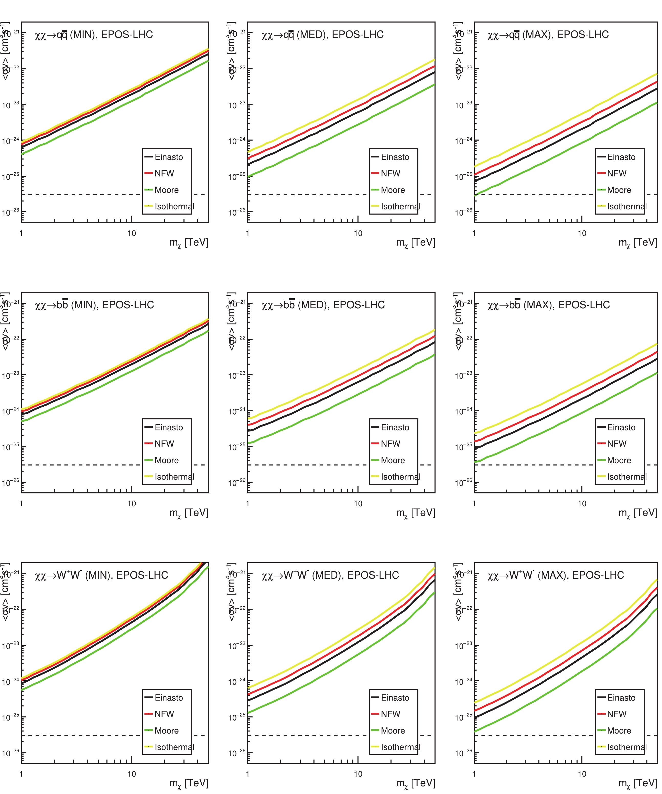
Figure 3. (color online) 95% CL upper limit of DM annihilation cross-sections as functions of DM particle masses, for different decay channels, propagation models and DM profiles, obtained by using the AMS-02
$ \bar{p}/p $ data [11] and the HAWC$ \bar{p}/p $ upper limit [32]. The energy spectrum of the secondary$ \bar{p} $ are calculated by the EPOS-LHC MC generator.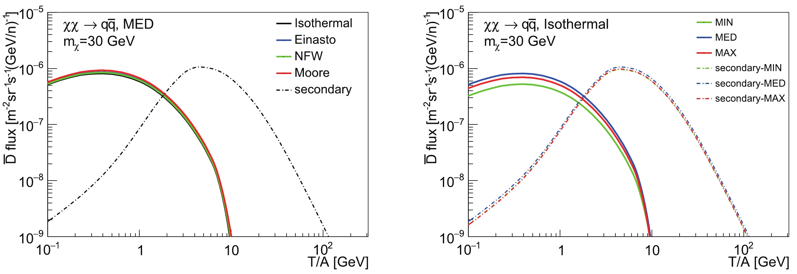
Figure 4. (color online) Comparisons of the maximal
$ \overline{\text{D}} $ fluxes for different propagation models and DM profiles, with DM annihilation into$ q\bar q $ final states and DM mass$ m_{\chi} = 30 $ GeV. The DM annihilation cross-sections are constrained by the AMS-02 and HAWC$ \bar{p}/p $ data, with the spectrum of secondary$ \bar{p} $ calculated using EPOS-LHC. (Left) Flux results in the "MED" propagation model with four different DM profiles. (Right) Flux results in three different propagation models, with DM profile fixed to "Isothermal". The secondary background of the$ \overline{ \rm{D}} $ flux is generated by EPOS-LHC. -
The galactic center (GC) is a promising place for detecting DM interactions, because of the expected high DM density. The 10-year HESS
$ \gamma $ -ray data [34] focus on a small area around the galactic center, and constrains the DM annihilation cross-sections well for “Cuspy” type DM profiles, which have a large gradient at the inner galactic halo. These include the "Einasto" profile and the "NFW" profile. For DM mass$ m_{\chi} \gtrsim 1 $ TeV, the galactic center$ \gamma $ -ray can place more stringent upper limits than the$ \bar{p}/p $ data. However, for “Cored” type DM profiles, which are flat near the galactic center, such as the "Isothermal" profile, the constraints from the$ \gamma $ -ray data are relatively weak.The latest galactic center
$ \gamma $ -ray analysis, with 254 hours' exposure, was published in 2016 by HESS [34]. The upper limits are calculated for several DM profiles and DM annihilation channels, but the$ \gamma $ -ray flux data have not been publicly released. Since the relative statistical error of a data point is inversely proportional to the square root of the number of counts in the bins, we can approximately estimate the 254-hour results by rescaling previous HESS$ \gamma $ -ray data [33], which were published in 2011 and for which exposure time was 112 hours. To obtain the upper limits for other DM profiles and channels, we perform a$ \chi^2 $ analysis to the 112-hour$ \gamma $ -ray flux data and estimate the 254-hour results by rescaling the data errors by a factor$ \sqrt{112/254} $ . The flux residual is defined as$ R^{\mathrm{exp}} = F^{\mathrm{exp}}_{\mathrm{Sr}}-F^{\mathrm{exp}}_{\mathrm{Bg}} $ , where$ F^{\mathrm{exp}}_{\mathrm{Sr}} $ and$ F^{\mathrm{exp}}_{\mathrm{Bg}} $ are the experimental$ \gamma $ -ray flux data from the source region and from the background region respectively, and the error of$ R^{\mathrm{exp}} $ is provided in Ref. [33].$ R^{\mathrm{th}} = F^{\mathrm{th}}_{\mathrm{Sr}}-F^{\mathrm{th}}_{\mathrm{Bg}} $ is the theoretical value of the flux residual, and the differential flux$ F^{\mathrm{th}} $ is calculated by the following formula:$ F^{\mathrm{th}} = \frac{\mathrm{d}\Phi_{\gamma}}{\Omega\mathrm{d}E_{\gamma}} = \frac{\langle\sigma v\rangle}{8\pi m_{\chi}^2\Omega}\frac{\mathrm{d} N_{\gamma}}{\mathrm{d}E_{\gamma}} \int_{\Omega}\int_{\mathrm{l.o.s}}\rho^2(r(s,\theta))\mathrm{d}s \mathrm{d}\Omega, $

(12) where
$ \mathrm{d} N_{\gamma}/\mathrm{d}E_{\gamma} $ is the energy spectrum of photons produced in one DM annihilation, and$ \Omega $ is the total spherical angle of the source or background regions. We adopt the reflected background technique described in Ref. [33] to determine the source region and background regions, and calculate the flux residual to perform the$ \chi^2 $ analysis. We randomly choose 540 pointing positions near the GC, with the maximal distance between the pointing position and the GC being$ 1.5^{\circ} $ . We first calculate the minimal$ \chi^2 $ value, and then the 95% CL upper limit corresponds to$ \Delta\chi^2 = 3.84 $ . The results are shown in Fig. 5. We can see that there are large gaps between the upper limits for different DM profiles. As expected, the constraints are stringent for DM profiles that are cuspy at the GC, but for a cored one like the Isothermal profile, the limits are rather weak. For various DM profiles, the constraints from$ \bar{p}/p $ data are are similar, because the DM densities in the diffusion halo are similar in different DM profiles, except for the GC region. However, for$ \gamma $ -ray data, the GC region provides the most stringent constraints for heavy DM particles, which leads to the large gaps between DM profiles.
Figure 5. (color online) 95% CL upper limit of DM annihilation cross-sections for different annihilation channels and DM profiles, obtained by using the HESS GC
$ \gamma $ -ray data with 112 hours' exposure [33]. The 254-hour results are derived by rescaling the data errors.We compare the upper limits from the
$ \bar{p}/p $ data and from the$ \gamma $ -ray data, as presented in Fig. 6. We use the "MED" propagation model as the benchmark model, and the "Isothermal" and "Einasto" profiles represent the typical "Cored" and "Cuspy" profiles respectively. The "Isothermal" profile is parameterized as follows: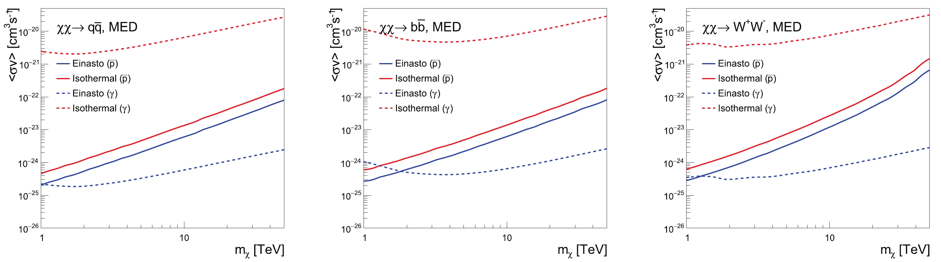
Figure 6. (color online) Comparison between the upper limits from the AMS-02 and HAWC
$ \bar{p}/p $ data and the HESS 254-hour GC$ \gamma $ -ray data. The solid lines stand for constraints from the$ \bar{p}/p $ data, and the dashed lines are the$ \gamma $ -ray limits. The "MED" propagation model is used as a benchmark model.$ \rho_{\mathrm{DM}} = \rho_{\odot}\frac{1+(r_{\odot}/r_{\mathrm{Iso}})^2}{1+(r/r_{\odot})^2}\; , $

(13) where
$ \rho_{\odot} = 0.43\; \mathrm{GeV/cm}^{3} $ is the local DM energy density,$ r_{\mathrm{Iso}} = 3.5\; \mathrm{kpc} $ . The "Einasto" profile can be written as:$ \rho_{\mathrm{DM}} = \rho_{\odot}\exp\left[-\left(\frac{2}{\alpha}\right)\left(\frac{r^{\alpha}- r^{\alpha}_{\odot}}{r^{\alpha}_{\mathrm{Ein}}}\right)\right]\; , $

(14) where
$ \alpha = 0.17 $ and$ r_{\mathrm{Ein}} = 20 $ kpc. As we can see, in all annihilation channels, for the "Isothermal" profile, the upper limits from$ \bar{p}/p $ data are much more stringent than those from the$ \gamma $ -ray data, while for the "Einasto" profile, the$ \gamma $ -ray data give stricter limits than$ \bar{p}/p $ for DM mass larger than 2 TeV.It is worth mentioning that the Fermi-LAT experiment [59] also collected a large amount of
$ \gamma $ -ray data near the GC, and the relatively large region of interest can reduce the large gaps between different DM profiles. However, the energy range of Fermi-LAT observations (from 20 MeV to more than 300 GeV) is much lower than that of HESS, and thus provides a weaker limitation on large DM mass. For example, the analysis in Ref. [60] shows that for a steep profile like “NFW”, HESS gives stronger constraints than Fermi-LAT at$ E\gtrsim1 $ TeV. For a flat profile like “Isothermal”, the Fermi-LAT limits derived in Ref. [61] are slightly weaker than the$ \bar{p}/p $ constraints at$ E\approx 10 $ TeV. From these facts, to make the most conservative conclusion, we use the$ \bar{p}/p $ limits to calculate the maximal$ \overline{\text{D}} $ and$ ^3\overline{\text{He}} $ fluxes in the “Isothermal” profile, and use the HESS$ \gamma $ -ray limits for the “Einasto” profile in the following sections. -
With the DM annihilation cross-section upper limits to hand, we can derive the maximal
$ \overline{\text{D}} $ and$ ^3\overline{\text{He}} $ fluxes for different annihilation channels, propagation models, and DM profiles. As shown in Fig. 4, by constraining the DM annihilation cross-section with the$ \bar{p}/p $ data, the uncertainties from the propagation models are small. We thus present our results for the “MED” propagation model, and other models do not affect our conclusions. For illustrative purposes, the particle mass of the heavy DM is set to be$ m_{\chi} = 10 $ and 50 TeV, which is smaller than the unitarity bound for a self-conjugate DM [62]. However, it is worth mentioning that our analysis is largely model-independent, and we do not assume that DM has thermal origins.Currently, the AMS-02 detector has the strongest detection ability for both
$ \overline{\text{D}} $ and$ ^3\overline{\text{He}} $ . For the$ \overline{\text{D}} $ flux, the AMS-02 detection sensitivity is given in Ref. [39], while the sensitivity for$ ^3\overline{\text{He}} $ has only been released in terms of the$ ^3\overline{\text{He}}/\mathrm{He} $ ratio in Ref. [20]. To study the detection prospects of AMS-02, we present our results in terms of$ \overline{\text{D}} $ fluxes and$ ^3\overline{\text{He}}/\mathrm{He} $ ratios.The results for the “Isothermal” profile with
$ m_{\chi} = 10 $ and 50 TeV are presented in Fig. 7, with the DM annihilation cross-section constrained by the AMS-02 and HAWC$ \bar{p}/p $ data. The top three figures show the results for$ \overline{\text{D}} $ fluxes for different annihilation channels, while the bottom three figures present the$ ^3\overline{\text{He}}/\mathrm{He} $ ratio results. The blue shaded areas represent the prospective AMS-02 detection sensitivity after 18 years of data collection, and the error bands show the uncertainties from coalescence momenta. Note that for$ \overline{\text{D}} $ , the error bands for the secondary background are thinner than the line width. We can see that for$ \overline{\text{D}} $ , the DM contributions exceed the secondary backgrounds in the energy region$ T/A\gtrsim300 $ GeV. For$ b\bar{b} $ and$ W^+W^- $ channels and$ m_{\chi} = 50 $ TeV, the excess can be as large as one order of magnitude. Similarly, for$ ^3\overline{\text{He}} $ , the excess exists at a kinetic energy of around 800 GeV per nucleon, and the primary$ ^3\overline{\text{He}} $ fluxes originating from DM annihilation can be 20 times larger than the secondary background with$ m_{\chi} = 50 $ TeV. Despite the fluxes of these anti-nuclei being small at high kinetic energies, and far below the AMS-02 sensitivities, these excesses can be promising windows for future detections.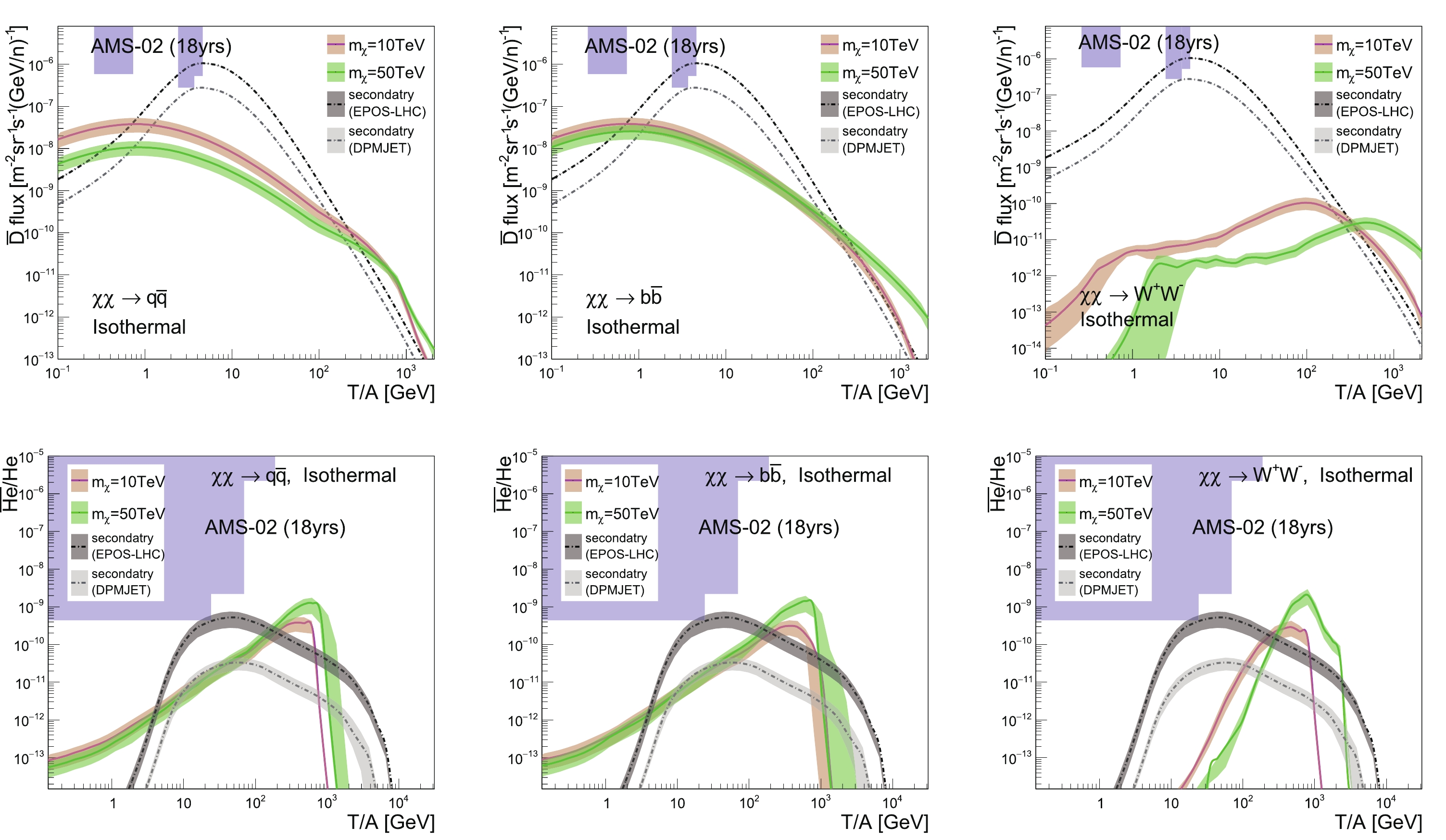
Figure 7. (color online)
$ \overline{\text{D}} $ fluxes (top figures) and$ ^3\overline{\text{He}}/\mathrm{He} $ ratios (bottom figures), for the “Isothermal” profile with large DM mass and the “MED” propagation model. The DM annihilation cross-section is constrained by the AMS-02 and HAWC$ \bar{p}/p $ data. The blue shaded areas represent the 18-year AMS-02 detection sensitivity.The results for the “Einasto” profile are shown in Fig. 8, with the DM annihilation cross-sections constrained by the HESS 10-year GC
$ \gamma $ -ray data. For$ \overline{\text{D}} $ , the DM contributions are below the secondary background in all energy regions and annihilation channels, and thus the high energy window closes. However, for$ ^3\overline{\text{He}} $ , the conclusion depends on the choice of MC generators. The DM contributions are lower than the secondary background given by EPOS-LHC, but can still exceed the DPMJET-III background.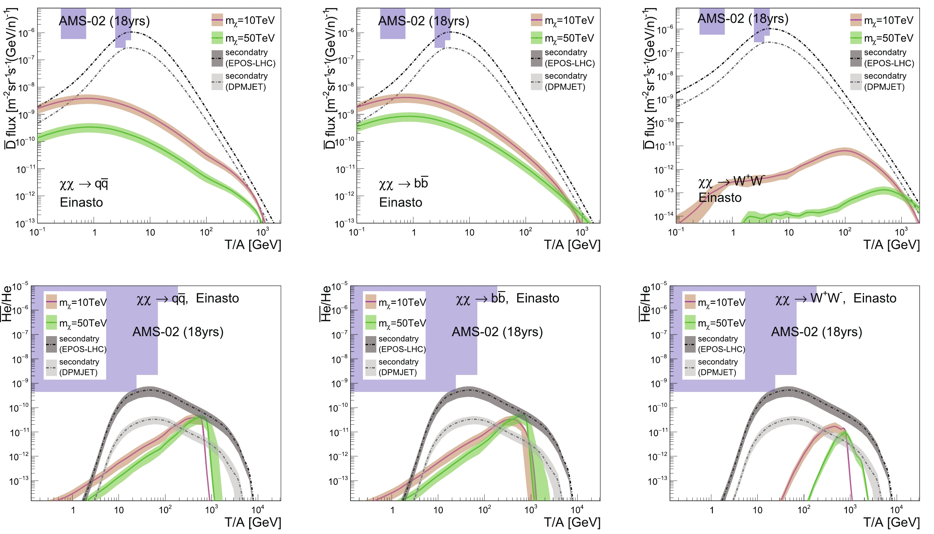
Figure 8. (color online)
$ \overline{\text{D}} $ fluxes (top figures) and$ ^3\overline{\text{He}}/\mathrm{He} $ ratios (bottom figures), for the “Einasto” profile with large DM mass and the “MED” propagation model. The DM annihilation cross-section is constrained by the HESS 10-year GC$ \gamma$ -ray data. The blue shaded areas represent the 18-year AMS-02 detection sensitivity. -
We also consider the process
$ \chi\chi \rightarrow \phi\phi \rightarrow f\bar{f}f\bar{f} $ , where two DM particles first annihilate into a couple of mediators, and then the mediators decay into standard model final states. If the mass of the mediator is much smaller than that of the DM particle, the mediator will be highly boosted. The$ \overline{\text{D}} $ and$ ^3\overline{\text{He}} $ produced in this process are thus expected to assemble in high energy regions, which provides a high signal-to-background ratio for the high energy window.By following the steps described in Sec. IV, we obtain the 95% CL upper limit of cross-sections for the annihilation process with mediators. The results for mediator mass
$ m_{\phi} = 200 $ GeV are presented in Fig. 9. Similar to the results for direct annihilations, for the “Isothermal” profile, the most stringent constraints are from$ \bar{p}/p $ data, while for the “Einasto” profile, the$ \gamma $ -ray limitations are stricter. Again, we use the AMS-02 and HAWC$ \bar{p}/p $ data to constrain the “Isothermal” profile, and the “Einasto” profile is restricted by the HESS GC$ \gamma $ -ray data.
Figure 9. (color online) 95% CL upper limit of DM annihilation cross-sections for different mediator decay channels. The solid lines are derived by using the AMS-02
$ \bar{p}/p $ data and the HAWC$ \bar{p}/p $ upper limit, while the dashed lines represent the limits from the HESS GC$ \gamma $ -ray data. The energy spectra of the secondary$ \bar{p} $ are calculated by EPOS-LHC, and the “MED” propagation model is used.The results for the “Isothermal” profile and “Einasto” profile with
$ m_{\phi} = 200 $ GeV are presented in Fig. 10 and Fig. 11 respectively. As expected, the DM contributions are boosted to high energy regions, and we get similar conclusions as in the direct annihilation channels. For the “Isothermal” profile with$ m_{\chi} = 50 $ TeV, the high energy window opens for both$ \overline{\text{D}} $ and$ ^3\overline{\text{He}} $ in all decay channels, especially for$ ^3\overline{\text{He}} $ , where the excesses can reach two orders of magnitude in the$ q\bar{q} $ and$ b\bar{b} $ channels. For$ m_{\chi} = 10 $ TeV, the DM contributions for$ \overline{\text{D}} $ and$ ^3\overline{\text{He}} $ are comparable to the secondary backgrounds.
Figure 10. (color online)
$ \overline{\text{D}} $ fluxes (top figures) and$ ^3\overline{\text{He}}/\mathrm{He} $ ratios (bottom figures), for the “Isothermal” profile and different mediator decay channels, with the “MED” propagation model. The DM annihilation cross-section is constrained by the AMS-02 and HAWC$ \bar{p}/p $ data.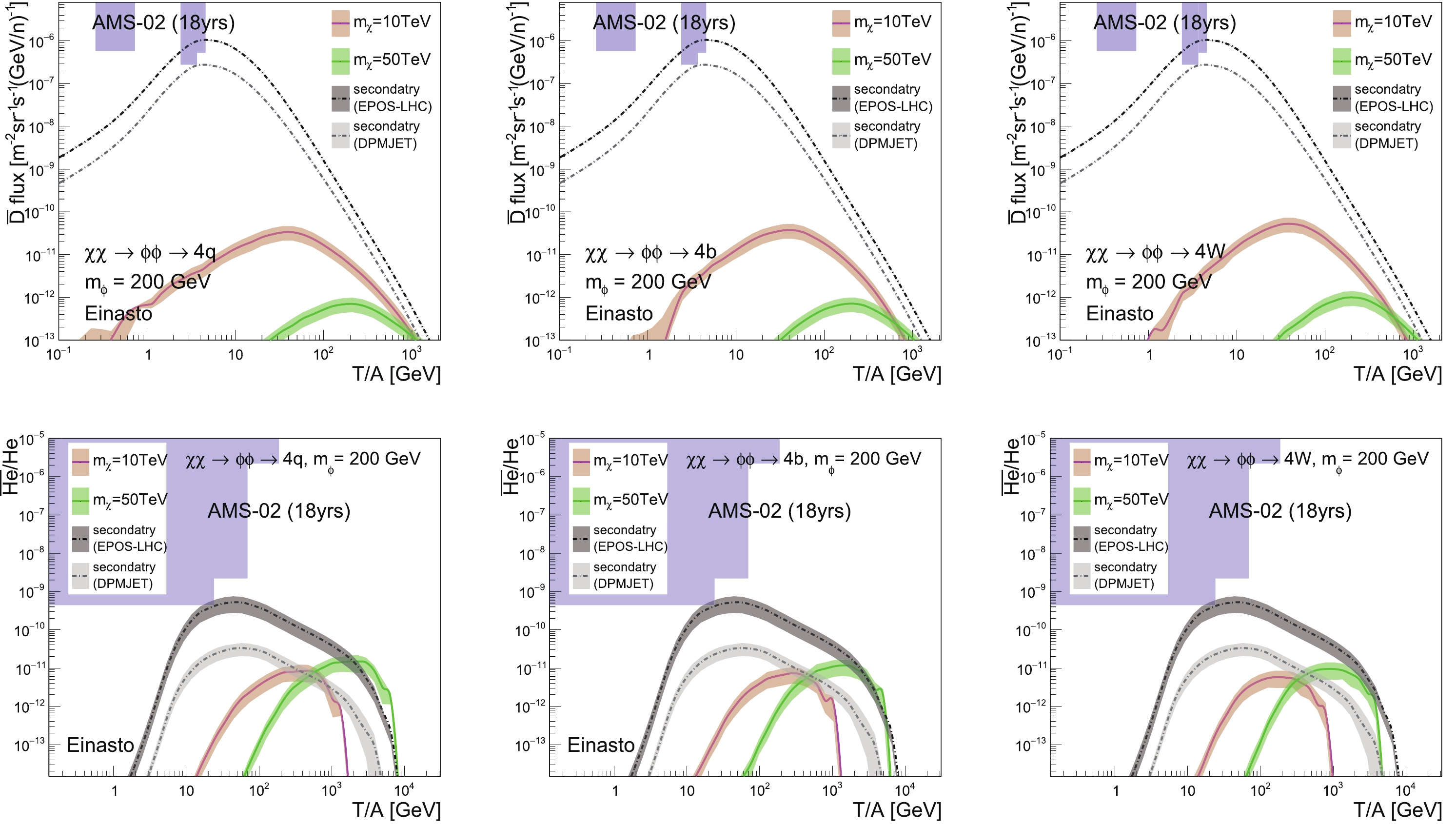
Figure 11. (color online)
$ \overline{\text{D}} $ fluxes (top figures) and$ ^3\overline{\text{He}}/\mathrm{He} $ ratios (bottom figures), for the “Einasto” profile and different mediator decay channels, with the “MED” propagation model are used. The DM annihilation cross section is constrained by the HESS 10-year GC$ \gamma $ -ray data.However, as shown in Fig. 11, for the “Einasto” profile, the excesses in high energy regions disappear for
$ \overline{\text{D}} $ for all DM masses and mediator decay channels. For$ ^3\overline{\text{He}} $ , the contributions from DM with$ m_{\chi} = 50 $ TeV can be larger than the background calculated by using DPMJET-III. For EPOS-LHC, however, the only excess appears in the$ q\bar{q} $ decay channel with$ m_{\chi} = 50 $ TeV.For other mediator masses, we reach the same conclusion. Taking the
$ \chi\chi \rightarrow \phi\phi \rightarrow 4q $ channel as an example, we calculate the$ \overline{\text{D}} $ fluxes and$ ^3\overline{\text{He}} $ ratios for mediator mass$ m_{\phi} = 60 $ , 200 and 600 GeV, and present the results for the “Isothermal” profile in Fig. 12. It can be seen that with the growth of the mediator mass, the DM contributions in low energy regions increase significantly. However, in high energy regions, in which we are interested, the variations of the results are small.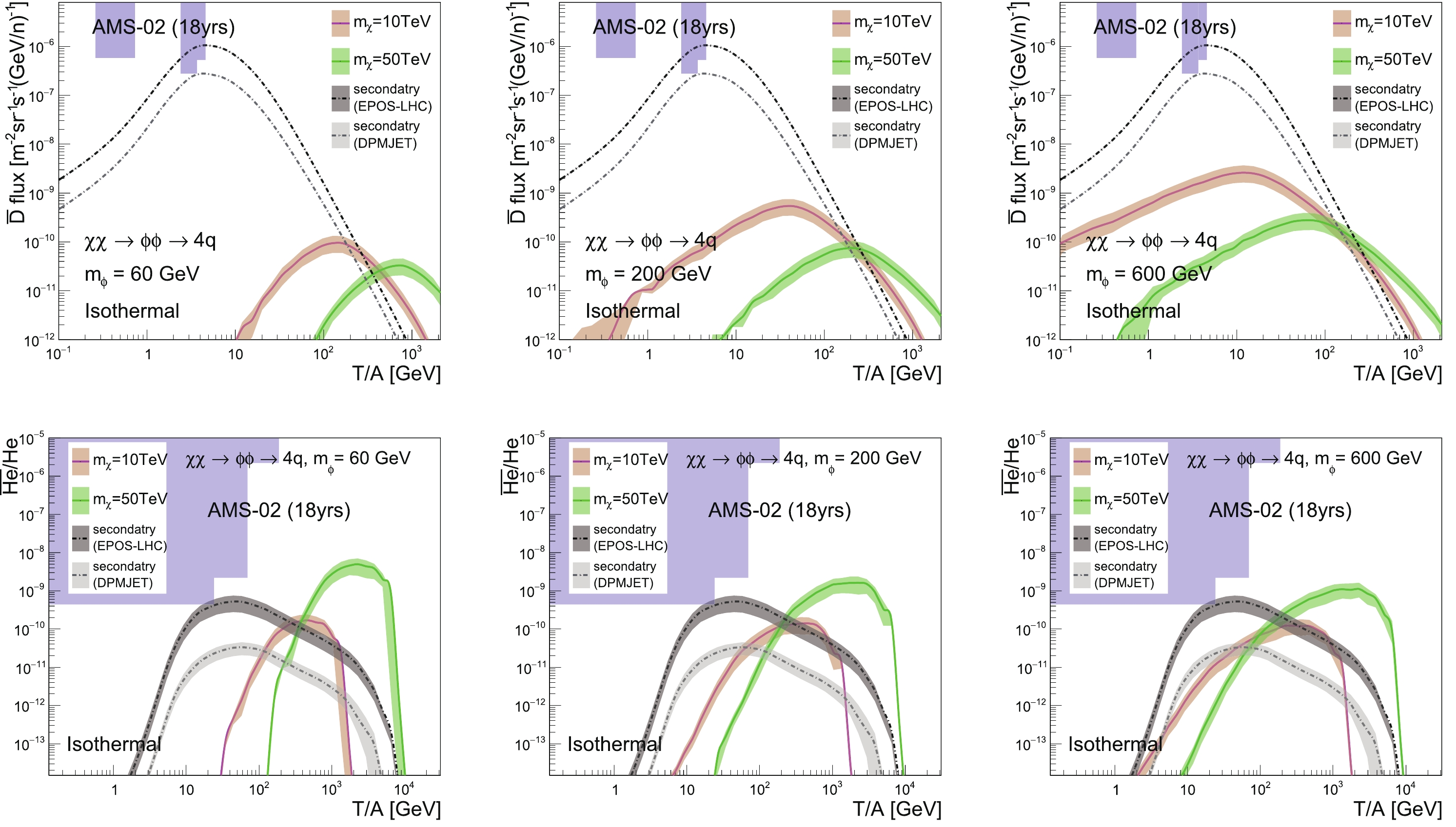
Figure 12. (color online)
$ \overline{\text{D}} $ fluxes (top figures) and$ ^3\overline{\text{He}}/\mathrm{He} $ ratios (bottom figures), for the “Isothermal” profile and$ \chi\chi \rightarrow \phi\phi \rightarrow 4q $ channels, with different mediator masses and the “MED” propagation model. The DM annihilation cross-section is constrained by the AMS-02 and HAWC$ \bar{p}/p $ data. -
In summary, we have explored the possibility of probing DM by high energy CR anti-nuclei. We used the MC generators PYTHIA 8.2, EPOS-LHC and DPMJET-III and the coalescence model to calculate the spectra of anti-nuclei. The coalescence momenta of
$ \overline{\text{D}} $ and$ ^3\overline{\text{He}} $ were derived by fitting the data from ALICE, ALEPH and CERN ISR experiments. The propagation of charged CR particles was calculated by the GALPROP-v54 code, with the inelastic interaction cross-sections between the primary CR and interstellar gases given by MC generators. We used the HESS GC$ \gamma $ -ray data to constrain the DM annihilation cross-sections for the DM profiles with large gradient at GC, while the flat profiles were limited by the AMS-02 and HAWC$ \bar{p}/p $ data.Our results showed that, for a “Cored” type DM density profile like the “Isothermal” profile, the high energy window opened for both
$ \overline{\text{D}} $ and$ ^3\overline{\text{He}} $ in all channels. However, for a “Cuspy” type profile like the “Einasto” profile, the$ \overline{\text{D}} $ contributions from DM annihilations were below the secondary background in both DM direct annihilation and annihilation through mediator decay channels. For$ ^3\overline{\text{He}} $ , the conclusion depended on the choice of MC generators. The$ ^3\overline{\text{He}} $ flux originating from DM annihilations could exceed the secondary background for DPMJET-III, while the excess disappeared for EPOS-LHC.Signals in high energy regions can effectively avoid the uncertainties from the solar activities. Although the fluxes of
$ \overline{\text{D}} $ and$ ^3\overline{\text{He}} $ in high energy regions are far below the sensitivity of current experiments like AMS-02 and GAPS, the high energy window could be a promising probe of DM for next-generation experiments. We believe that with the fast development of detector technologies, DM detection through the high energy window will eventually be possible.
High energy window for probing dark matter with cosmic-ray antideuterium and antihelium
- Received Date: 2021-02-20
- Available Online: 2021-06-15
Abstract: Cosmic-ray (CR) anti-nuclei are often considered important observables for indirect dark matter (DM) detection at low kinetic energies, below GeV per nucleon. Since the primary CR fluxes drop quickly towards high energies, the secondary anti-nuclei in CR are expected to be significantly suppressed in high energy regions (


 DownLoad: