


 Abstract
 HTML
HTML Reference
 Related
 PDF
PDF


-
The doubly heavy baryons with two heavy flavor quarks (the b or c quark) were predicted by the quark model and quantum chromodynamics (QCD) several decades ago [1-3]. Their structure, analogous to a heavy double-star system with an attached light planet [4], is very different from single-heavy-flavor baryons and light baryons. Furthermore, research on the doubly heavy baryons is a powerful tool in investigations of doubly and fully heavy tetraquark states [5, 6]. Therefore, the doubly heavy baryons open a new window for research on the properties of QCD [7].
However, there have been many twists and turns in the history of experimental searches for doubly heavy baryons. In 2002,
$ \Xi_{cc}^+ $ was first reported as observed by the SELEX collaboration via the mode of$ \Xi_{cc}^+\to\Lambda_c^+K^-\pi^+ $ [8]. None of the following measurements by FOCUS [9], BaBar [10], Belle [11], and LHCb [12] found signatures using the same decay mode. Actually, the production rate of the doubly charmed baryons was large enough at the beginning of LHCb running [13, 14]. The remaining problem is the decay properties, i.e. which decay processes have the largest branching fractions and final particles which can easily be detected in the experiments [15]. In 2017, a theoretical analysis of all the decay processes found that$ \Xi_{cc}^{++}\to\Lambda_c^+K^-\pi^+\pi^+ $ and$ \Xi_{c}^+\pi^+ $ are the most favorable for the discovery of doubly charmed baryons [16]. Subsequently, the LHCb collaboration observed the doubly charmed baryon for the first time via$ \Xi_{cc}^{++}\to\Lambda_c^+K^-\pi^+\pi^+ $ [17], following the theoretical suggestions, and confirmed the discovery via$ \Xi_{cc}^{++}\to\Xi_{c}^+\pi^+ $ in 2018 [18]. It is clear that theoretical studies of the decay properties play an important role in experimental searches for the doubly heavy baryons.There are two difficulties in theoretical calculations of the dynamics of doubly charmed baryon decays: charm decay with large non-perturbative contributions, and baryon decay with a three-body problem. For charm decays, QCD-inspired methods do not work well at scales of around 1 GeV. In the charmed meson decays, there are significant non-perturbative contributions to the topological amplitudes which are extracted from the experimental data of the decay branching fractions [19-23]. However, the topological diagrammatic approach cannot be directly used in doubly charmed baryon decays, since there are no available data. The charmed baryon decays are even more complicated [24-50]. As a first attempt to study non-leptonic doubly charmed baryon decays, in Ref. [16], the factorizable contributions were calculated under the factorization hypothesis, and the non-factorizable contributions calculated considering the rescattering mechanism of the final-state-interaction (FSI) effects. In this work, we will systematically illustrate this theoretical framework in the decays of doubly charmed baryons into a charmed baryon and a light pseudoscalar meson.
The success of the factorization and rescattering mechanism in suggesting the discovery channels of the doubly charmed baryons shows that the above framework roughly describes the correct dynamics of doubly charmed baryon decays. There is no doubt that the factorization approach works well for the short-distance tree-emitted diagrams [20, 21, 23, 51, 52]. The problem is how to calculate the long-distance contributions, which are usually considered as FSI effects. Much work has been done to calculate the FSI effects of weak decays of heavy-flavor mesons [53-60]. Before Ref. [16], there was no work on the long-distance contributions of doubly heavy baryon decays, and only a few works on the short-distance factorizable contributions [61, 62]. The non-perturbative contributions are very important in charm decays. The rescattering mechanism of the FSI effect was first investigated for
$ \Lambda_c^+ $ decays in Ref. [60], and first studied for doubly charmed baryon decays in Ref. [16].The theoretical framework of the rescattering mechanism is as follows. The doubly charmed baryon decays via a short-distance tree-emitted process into one baryon and one meson, which scatter with each other by exchanging one particle as a long-distance effect into the final states. It forms a triangle diagram at the hadron level. The short-distance and long-distance contributions are separated to avoid the double-counting problem. In this work, the calculation techniques follow Ref. [58], in which the cutting rules are used to compute the imaginary part of the triangle diagram. There is a basic difference between our framework and those of Refs. [54, 58]. The triangle diagrams of the rescattering mechanism are taken as an independent method by the calculation of hadron-level Feynman diagrams, while in Refs. [54, 58] the triangle diagrams are calculated corresponding to the quark topological diagrams. The problem of the latter method is discussed elsewhere [63].
FSI calculations suffer large theoretical uncertainties. The branching fractions could be changed by one order of magnitude with the variation of the non-perturbative parameters like
$ \eta $ in the form factor of the cutting rules or the cut-off$ \Lambda $ in the loop calculation. The parameters are always determined by the measured results of the branching fractions [54, 58]. However, in the case of doubly charmed baryons, there is no available data to determine the non-perturbative parameters. Therefore, the biggest problem in the FSI calculations is how to control the theoretical uncertainties. The innovation of our method is to calculate the ratios of branching fractions, which are not sensitive to the non-perturbative parameters. The uncertainties of the ratios are thus well under control. That is why Ref. [16] could correctly and reliably predict the modes with the largest branching fractions.Knowledge of the relative sizes of the topological diagrams of heavy baryon decays leads to important implications for the predictions of the most favorable modes to discover the doubly charmed baryons. In the soft-collinear effective theory [64, 65], the power counting rules of
$\dfrac{|C|}{|T|}\sim\dfrac{|C^\prime|}{ |C|}\sim\dfrac{|E_1|}{|C|}\sim\dfrac{|E_2|}{ |C|}\sim {O\left(\dfrac{\Lambda^h_{\rm{QCD}}}{ m_c}\right) }$ are obtained. These relations are manifested by the most precise measurements of the$ \Lambda_c^+ $ decays performed by the BESIII collaboration [66]. In addition, the discovery channel of$ \Xi_{cc}^{++}\to \Lambda_c^+K^-\pi^+\pi^+ $ dominated by$ \Xi_{cc}^{++}\to \Sigma_c^{++}\overline K^{*0} $ can be directly related to the result of$ \Lambda_c^+\to p\phi $ [67] by exactly the same topological diagram, with an interchange of a spectator quark. In this work, we will calculate the topological diagrams by the rescattering mechanism to test the above relations. The flavor$ SU(3) $ symmetry and its breaking effects will also be discussed. It has to be stressed that the weak decays of doubly charmed baryons have been widely studied [61, 62, 68-94], especially after the work of Ref. [16] and the experimental observation of$ \Xi_{cc}^{++} $ . The clarification of our framework will be helpful to understand the dynamics and nature of doubly charmed baryons.This paper is arranged as follows. In Sec. II, we introduce the theoretical framework of the rescattering mechanism and demonstrate the calculation details with
$ \Xi_{cc}^{++}\to\Xi_c^+\pi^+ $ as an example. Then the parameter inputs, numerical results of branching fractions and relevant discussions are presented in Sec. III. At the end, we give a brief summary. The effective hadron-strong-interaction Lagrangians and corresponding strong coupling constants are collected in Appendix A. The expressions of the decay amplitudes for all the decay modes considered are gathered in Appendix B. -
The exclusive non-leptonic weak decays of doubly charmed baryons are induced by the charge currents of charm decays at the tree level. The penguin contributions are safely neglected in the branching fractions of charm decays, due to the smallness of the corresponding CKM matrix elements. The effective Hamiltonian is given by
$ \begin{aligned}[b]{\cal{H}}_{\rm eff} =& \frac{G_F}{\sqrt{2}}\sum\limits_{q^{\prime} = d,s}^{}V_{cq^{\prime}}^\ast V_{uq}[C_1(\mu)O_1(\mu)\\&+C_2(\mu)O_2(\mu)]+{\rm h.c}.. \end{aligned}$

(1) with the four-fermion operators of
$ \begin{aligned}[b] O_1 =& (\bar{u}_\alpha q_\beta)_{V-A}(\bar{q^{\prime}}_\beta c_\alpha)_{V-A},\\ O_2 = &(\bar{u}_\alpha q_\alpha)_{V-A}(\bar{q^{\prime}}_\beta c_\beta)_{V-A}, \end{aligned} $

(2) where
$ q^{(\prime)} = (s,d) $ ,$ \alpha $ and$ \beta $ are color indices,$ V_{cq^{\prime}} $ and$ V_{uq} $ are the Cabibbo-Kobayashi-Maskawa (CKM) matrix elements, and$ G_F = 1.166\times 10^{-5}\rm{ GeV}^{-2} $ is the Fermi constant.$ C_{1,2}(\mu) $ denote the Wilson coefficients, which include the short-distance QCD dynamics scaling from$ \mu = M_W $ to$ \mu = m_c $ . To obtain the amplitudes of$ {\cal{B}}_{cc}\to{\cal{B}}_cP $ decays, one needs to evaluate the next hadronic matrix element of the effective Hamiltonian:$\langle{\cal{B}}_cP|{\cal{H}}_{\rm eff}|{\cal{B}}_{cc}\rangle = \frac{G_F}{\sqrt{2}}V^{\ast}_{cq^{\prime}}V_{uq}\sum\limits_{i = 1,2}C_i\langle{\cal{B}}_cP|O_i|{\cal{B}}_{cc}\rangle. $

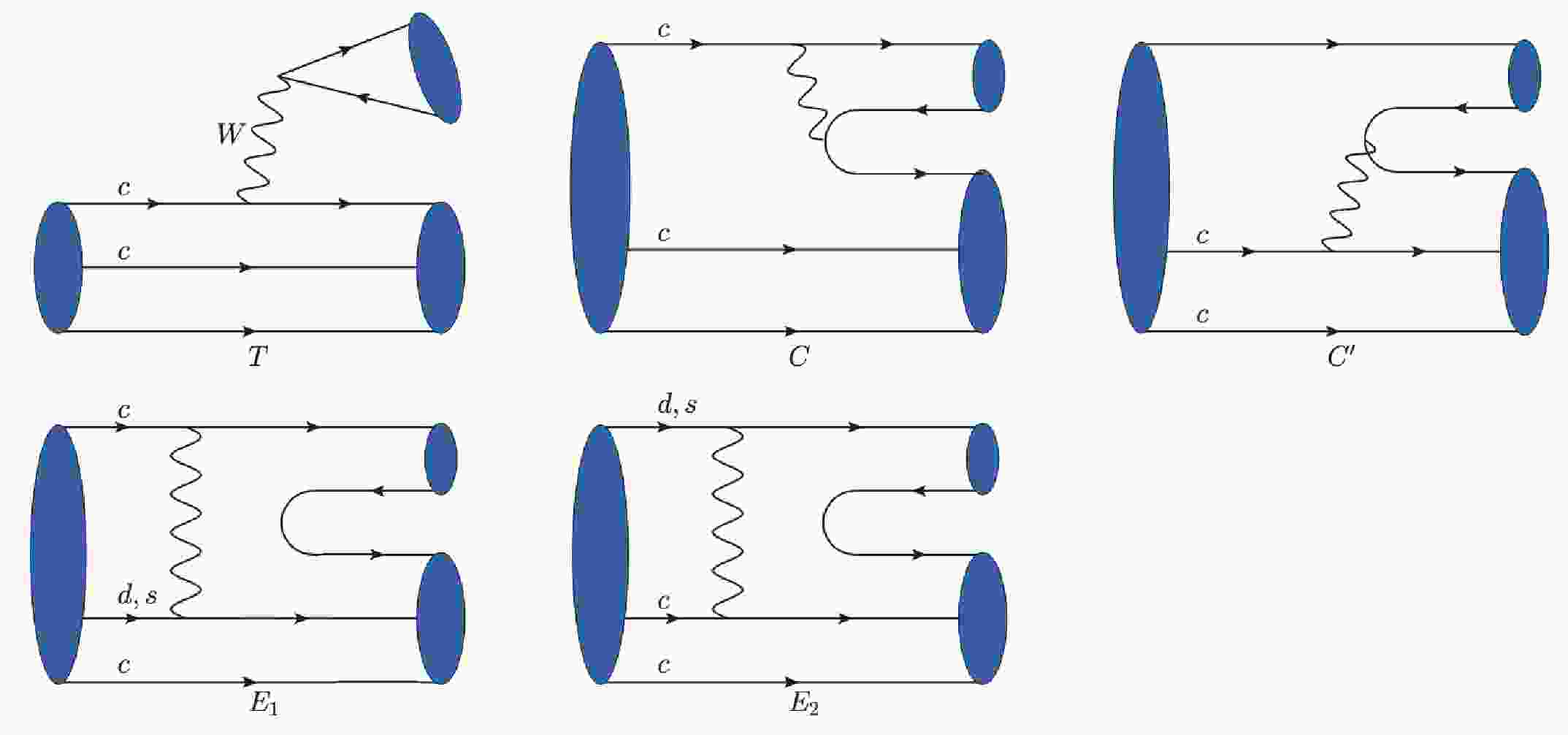
(3) The general tree-level topological diagrams of doubly charmed baryons decaying into a singly charmed baryon and a light meson are displayed in Fig. 1. These diagrams can be sorted by their different topologies. Each diagram contains both short-distance and long-distance contributions. T describes the color-allowed external W-emission diagram, while C and
$ C^\prime $ can both be used to represent color-suppressed internal W-emission diagrams. The C diagram is the one with both the quark and anti-quark of the final light meson state coming from the weak vertex, while for$ C^\prime $ only the antiquark is generated from the weak vertex and the quark is directly transferred from the light spectator of the doubly charmed baryon. There are also two different types of W-exchange diagrams, labeled$ E_1 $ and$ E_2 $ . In$ E_1 $ , the light quark produced by the charmed quark decay is absorbed into the light mesons. In$ E_2 $ , the light quark produced from the charmed quark decay is absorbed into a singly heavy baryon. The possible quark loop (penguin) diagrams relevant to the tree-level topological diagrams also have a non-negligible impact on the estimation of the long-distance contributions in our framework.
Figure 1. (color online) Tree-level topological diagrams for two-body non-leptonic decays of the doubly charmed baryons
${\cal{B}}_{cc} =({\Xi_{cc}^{++}},{\Xi_{cc}^+},{\Omega_{cc}^+})$ to a singly heavy baryon${\cal{B}}_c$ with a light pseudoscalar meson$P=(\pi, K, \eta_1,\eta_8)$ .In the calculation of these topological diagrams, it has been demonstrated that T is dominated by factorizable contributions [95] and can be calculated under the factorization hypothesis. However, this factorizable contribution of the C diagram is heavily suppressed by the color factor at charm scale, with the effective Wilson coefficient
$ a_2(m_c) = C_1(m_c)+C_2(m_c)/N_c $ . The factorizable short-distance contributions are therefore negligible, but the long-distance dynamics of C can play an important role [16]. The short-distance amplitudes of topological diagrams$ C^\prime $ ,$ E_1 $ and$ E_2 $ are also expected to be suppressed at least by one order [95], while the long distance dynamics is more important at the scale of the charm quark mass.In the following sections, we take the second discovery channel
$ \Xi_{cc}^{++}\to\Xi_c^+\pi^+ $ [16, 18] as an example to introduce our framework in detail. This decay contains two contributions of topological amplitude, i.e.$ T+C^\prime $ , in which T is dominated by the short-distance dynamics, while$ C^\prime $ is dominated by the non-factorizable long-distance dynamics. T usually plays the central role compared with$ C^\prime $ (mainly due to the colour suppression). However, from our calculation, it can be seen that the non-factorizable contributions of$ C^\prime $ may have a significant impact on the total amplitude. -
In this section, we discuss how to calculate the factorizable short-distance contributions of the topological amplitudes T and C. The feasible approach is the factorization approach, with the matrix elements
$ \langle{\cal{B}}_cM|O_i|{\cal{B}}_{cc}\rangle $ in Eq. (3) factorized into the product of two parts. One is parameterized as the decay constant of the emitted mesons and the other is expressed as the transition form factors. The factorizable contribution of the T diagram is expressed as:$\begin{aligned}[b] \langle{\cal{B}}_{c}M|{\cal{H}}_{\rm eff}|{\cal{B}}_{cc}\rangle_{SD}^T = \frac{G_F}{\sqrt{2}}V^\ast_{cq^\prime}V_{uq}a_1(\mu)\langle M|\bar{u}\gamma^\mu(1-\gamma_5)q|0\rangle\langle {\cal{B}}_c|\bar{q}^\prime\gamma_\mu(1-\gamma_5)c|{\cal{B}}_{cc} \rangle ,\end{aligned} $ 
(4) while the factorizable C diagram is given by
$\begin{aligned}[b] \langle{\cal{B}}_{c}M|{\cal{H}}_{\rm eff}|{\cal{B}}_{cc}\rangle_{SD}^C = \frac{G_F}{\sqrt{2}}V^\ast_{cq^\prime}V_{uq}a_2(\mu)\langle M|\bar{q}^\prime\gamma^\mu(1-\gamma_5)q|0\rangle\langle{\cal{B}}_c|\bar{u}\gamma_\mu(1-\gamma_5)c|{\cal{B}}_{cc}\rangle,\end{aligned}$

(5) where
$ a_1(a_2) $ represents the effective Wilson coefficients,$ a_1(\mu) = C_1(\mu)+C_2(\mu)/3 $ and$ a_2(\mu) = C_2(\mu)+C_1(\mu)/3 $ , with the Wilson coefficients$ C_1(\mu) = 1.21 $ and$ C_2(\mu) = -0.42 $ at the scale of charm decays$ \mu = m_c $ [21]. The meson M represents both the pseudoscalar and vector mesons, since, as will be seen in the next subsections, the vector meson contributes to the long-distance dynamics as an intermediate state.In both Eqs. (4) and (5), the first hadronic matrix element is parameterized in the same way, as:
$ \langle P(p)|\bar{u}\gamma^\mu(1-\gamma_5)q|0\rangle = -{\rm i}f_Pp^\mu, $

(6) $ \langle V(p)|\bar{u}\gamma^\mu(1-\gamma_5)q|0\rangle = m_Vf_V\epsilon^{\ast \mu}.$

(7) where
$ f_P $ and$ f_V $ are the corresponding decay constants of the pseudoscalar and vector mesons, and$ \epsilon^\mu $ denotes the polarization of the vector meson. The second matrix element is usually defined as:$ \begin{aligned}[b] \langle {\cal{B}}_c(p^\prime,s_z^\prime)| \bar{q}^{\prime}\gamma_\mu(1-\gamma_5)c |{\cal{B}}_{cc}(p,s_z)\rangle = & \bar u(p^\prime,s^\prime_z)\Big [ \gamma_\mu f_1(q^2)+{\rm i}\sigma_{\mu\nu}\frac{q^\nu}{M_{{\cal{B}}_{cc}}} f_2(q^2)+\frac{q^\mu}{M_{{\cal{B}}_{cc}}} f_3(q^2) \Big ] u(p,s_z) -\bar u(p^\prime,s^\prime_z)\\ & \times\Big [ \gamma_\mu g_1(q^2) + {\rm i}\sigma_{\mu\nu}\frac{q^\nu}{M_{{\cal{B}}_{cc}}}g_2(q^2) +\frac{q^\mu}{M_{{\cal{B}}_{cc}}} g_3(q^2) \Big ] \gamma_5 u(p,s_z). \end{aligned} $ 
(8) with
$ q = p-p^\prime $ ,$ M_{{\cal{B}}_{cc}} $ the mass of the doubly charmed baryon, and$ f_i $ ,$ g_i $ the heavy-light transition form factors, which can only be extracted from non-perturbative approaches.In general, the weak decay amplitudes of
$ {\cal{B}}_{cc}\to{\cal{B}}_c P $ and$ {\cal{B}}_c V $ have the following parametrization form:${\cal{A}}({\cal{B}}_{cc}\to{\cal{B}}_c P) = {\rm i}\bar{u}_{{\cal{B}}_c}(A + B\gamma_5) u_{{\cal{B}}_{cc}}, $

(9) $\begin{aligned}[b]{\cal{A}}({\cal{B}}_{cc}\to{\cal{B}}_c V) =& \epsilon^{\ast \mu}\bar{u}_{{\cal{B}}_c} \Bigg [ A_1\gamma_\mu\gamma_5 + A_2\frac{p_\mu({\cal{B}}_c)}{M_{{\cal{B}}_{cc}}}\gamma_5 \\&+B_1\gamma_\mu+B_2\frac{p_\mu({\cal{B}}_c)}{M_{{\cal{B}}_{cc}}} \Bigg ] u_{{\cal{B}}_{cc}}. \end{aligned}$

(10) The formulas of the parameters
$ A,B $ and$ A_{1,2},B_{1,2} $ under the factorization approach are:$\begin{aligned}[b] A =& \lambda f_P(M_{{\cal{B}}_{cc}}-M_{{\cal{B}}_{c}})f_1(m^2), \\ B =& \lambda f_P(M_{{\cal{B}}_{cc}}+M_{{\cal{B}}_{c}})g_1(m^2), \end{aligned}$

(11) $\begin{aligned}[b] A_1 =& -\lambda f_Vm \left ( g_1(m^2)+g_2(m^2)\frac{M_{{\cal{B}}_{cc}}-M_{{\cal{B}}_{c}}}{M_{{\cal{B}}_{cc}}} \right ), \\ A_2 =& -2\lambda f_Vmg_2(m^2), \end{aligned}$

(12) $\begin{aligned}[b] B_1 =& \lambda f_V m \left ( f_1(m^2)-f_2(m^2)\frac{M_{{\cal{B}}_{cc}}+M_{{\cal{B}}_{c}}}{M_{{\cal{B}}_{cc}}} \right ), \\ B_2 =& 2\lambda f_Vmf_2(m^2). \end{aligned}$

(13) where
$ \lambda = \dfrac{G_F}{\sqrt{2}}V_{\rm CKM}a_{1,2}(\mu) $ , and m is the mass of the pseudoscalar or vector meson. -
The long-distance contributions are important but not easy to evaluate. As is done in Ref. [16], we calculate the FSI effects by the rescattering of two intermediate particles at the hadron level using the hadronic strong-interaction effective Lagrangian. The diagram description of the rescattering mechanism is shown in Fig. 2. The weak vertex displayed in hadron-level diagrams only involves the short-distance contributions and thus can be evaluated under the factorization hypothesis. The subsequent scattering process could in principle be either a s-channel resonant-state process or a
$ t/u $ -channel one. The dominant contribution of the s-channel diagram comes from the momentum region$ k^2\sim m_{ \Xi_{cc}^+}^2 $ , which demands that the mass of the exchanged particle (a singly charmed baryon in this case) approaches$ m_{ \Xi_{cc}^+}\sim 3.6 $ GeV. However, the heaviest observed singly charmed baryons to date are much lighter than$ m_{ \Xi_{cc}^+} $ . Therefore, the s-channel diagram is usually highly suppressed by the off-shell effect and can be safely neglected. In our calculations, the main contribution will be the$ t/u $ -channel triangle diagram, as shown in Fig. 2.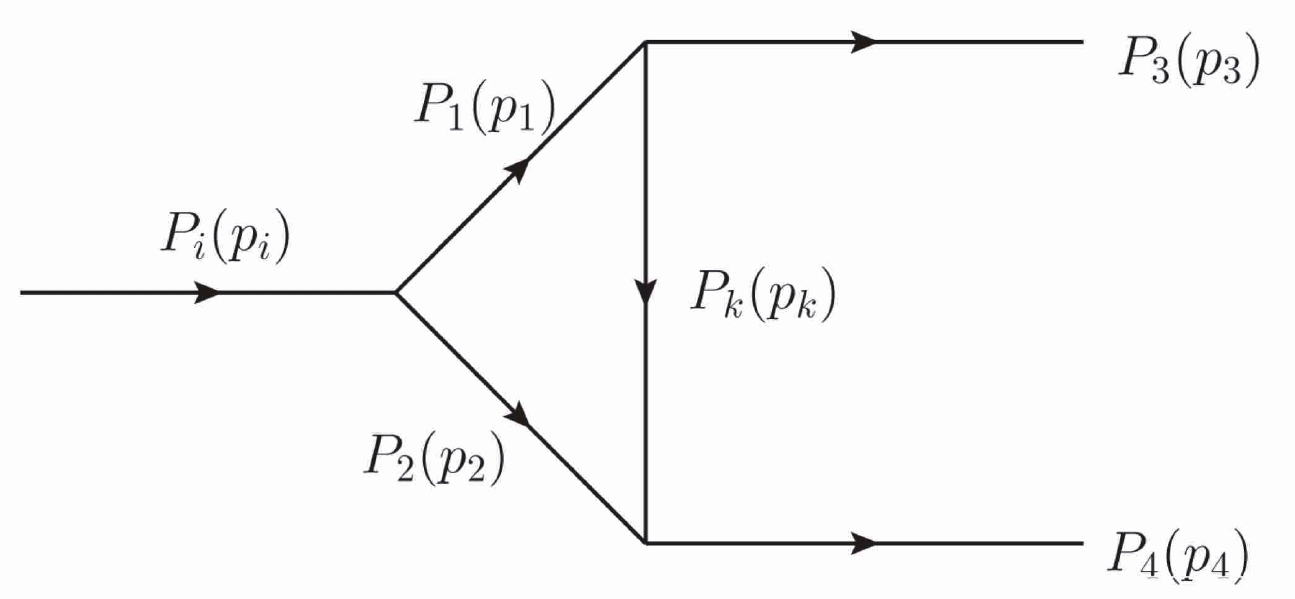
Figure 2. Diagram description of the rescattering mechanism at the hadron level.
The particles in the triangle diagram are labeled as
$ P_n $ , where the subscripts$ n = i,1,2,3,4,k $ represent the parent doubly charmed particle$ (i) $ , two intermediate hadrons$ (1,2) $ , two final hadron states$ (3,4) $ and the exchanged hadron$ (k) $ , respectively, as seen in Fig. 2. The corresponding momenta are assigned as$ p_n $ . In general, there are several methods to calculate the amplitude of a triangle diagram [53-59]. The main difference between them is the method of dealing with the hadronic loop integration.We adopt the optical theorem and Cutkosky cutting rule, as in Ref. [58]. The absorptive part of the amplitude of
$ P_i\to P_3P_4 $ is a product of two distinct parts, the decay of$ P_i\to \{P_1P_2\} $ and the rescattering of$ \{P_1P_2\}\to P_3P_4 $ , with the internal particles ($ P_1 $ and$ P_2 $ ) being on-shell. According to the optical theorem, the absorptive amplitude should sum over all possible on-shell intermediate states$ \{P_1P_2\} $ with a phase integration. It can be expressed as$ \begin{aligned}[b] {\cal{A}}bs [{\cal{M}}(P_i\to P_3P_4)] =& \frac{1}{2}\sum\limits_{\{P_1P_2\}} \int\frac{\rm{d}^3 p_1}{(2\pi)^3 2E_1}\int\frac{\rm{d}^3 p_2}{(2\pi)^3 2E_2}\\&\times(2\pi)^4 \delta^4(p_3 + p_4 - p_1-p_2) \\ &\times M(P_i\to\{P_1P_2\})T^*(P_3P_4\to\{P_1P_2\}). \end{aligned} $

(14) Based on the argument in Refs. [96, 97], the
$ 2 $ -body$ \rightleftharpoons $ n-body rescattering is negligible. In this approach, the loop integration is transferred into the dispersive part, which can be calculated via the dispersion relation${\cal{D}}is[ {\cal{M}}(m_1^2)] = \frac{1}{\pi}\int_s^\infty \frac{{\cal{A}}bs[{\cal{M}}(s^\prime)]}{s^\prime - m_1^2} \rm{d}s^\prime. $

(15) However, it suffers from large ambiguities, since we cannot reliably describe
$ {\cal{M}}(s') $ for the whole region. On the other hand, in the charmed meson decays, the large strong phases of the topological diagrams [20, 21] indicate that the absorptive (imaginary) part is dominant. Therefore, we will only calculate the absorptive part and neglect the dispersive part, as done in Ref. [58]. In a phenomenological analysis, the non-negligible dispersive contributions can be effectively absorbed into the varying of the parameter$ \eta $ , which will be introduced in the following.Next we express the amplitude of the decay mode
$ \Xi_{cc}^{++}\to\Xi_c^+\pi^+ $ as an example. All the rescattering diagrams are represented in Fig. 3, which can be summarized as$ \Xi_{cc}^{++}\to\Xi_c^+(\Xi_c^{\prime+}) \pi^+(\rho^+)\to\Xi_c^+\pi^+ $ . The intermediate particles can be either light pseudoscalar or vector mesons, or anti-triplet or sextet singly charmed baryons. We use the symbol$ {\cal{M}}(P_1,P_2;P_k) $ to denote a triangle amplitude with the intermediate states of$ P_1 $ ,$ P_2 $ and$ P_k $ .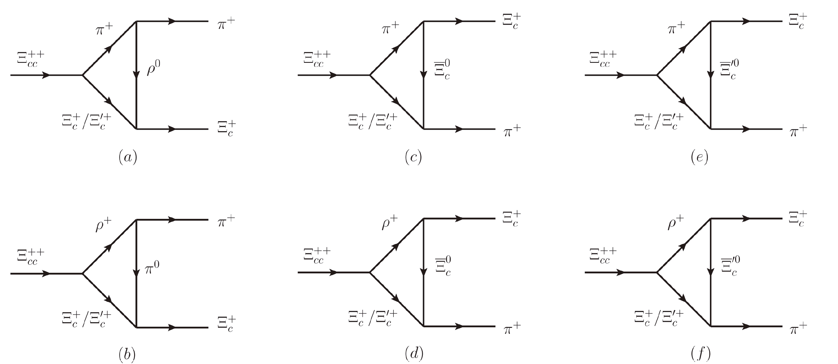
Figure 3. Long-distance rescattering contributions to
${\Xi_{cc}^{++}}\to\Xi_c^+\pi^+$ manifested at hadron level.Figure 3(a) contains two different triangle diagrams, with the intermediate two-particle states of
$ \{\Xi_c^+\pi^+\} $ and$ \{\Xi_c^{\prime+}\pi^+\} $ , respectively. The amplitudes of the weak vertex$ \Xi_{cc}^{++}\to\Xi_c^+\pi^+ $ and$ \Xi_{cc}^{++}\to\Xi_c^{'\prime}\pi^+ $ are taken from Eq. (9) in the factorization approach for the short-distance contributions. The rescattering amplitudes of$ \Xi_c^+\pi^+\to\Xi_c^{+}\pi^+ $ and$ \Xi_c^{\prime+}\pi^+\to\Xi_c^+\pi^+ $ can simply be found from the hadronic strong Lagrangian in Appendix A. Then the absorptive part is written as:$ \begin{aligned}[b] {\cal{A}}bs[{\cal{M}}(\pi^+,\Xi_c^+/\Xi_c^{\prime +};\rho^0)] =\;& \frac{1}{2}\sum\limits_{s_1,\lambda_k}\int\frac{{\rm d}^3\vec{p}_1}{(2\pi)^32E_1}\frac{{\rm d}^3\vec{p}_2}{(2\pi)^32 E_2}(2\pi)^4\delta^4(p_i-p_1-p_2) \\ & \times {\rm i} \bar{u}(p_4,s_4) \left(f_{1\rho^0(\Xi_c^+/\Xi_c^{\prime +})\to\Xi_c^+}\gamma_\nu-\frac{{\rm i}f_{2\rho^0(\Xi_c^+/\Xi_c^{\prime +})\to\Xi_c^+}}{2m_{\Xi_c^+}}\sigma_{\mu\nu}k^\mu\right) u(p_2,s_2)\epsilon^\nu(k,\lambda_k) \\ & \times \frac{F^2(t,m_{\rho})}{t-m_{\rho}^2+im_{\rho}\Gamma_{\rho}}(-{\rm i}g_{\pi^+\to\rho^0\pi^+})\epsilon^{\ast \alpha}(k,\lambda_k) (p_1+p_3)_\alpha \; i\bar{u}(p_2,s_2)(A+B\gamma_5)u(p_i,s_i) \\ =& \int\frac{|\vec{p}_1|{\rm sin}\theta {\rm d}\theta {\rm d}\phi}{32\pi^2m_{\Xi_{cc}^{++}}}\; {\rm i}^2(-{\rm i}g_{\pi^+\to\rho^0\pi^+}) \frac{F^2(t,m_{\rho})}{t-m_{\rho}^2+{\rm i}m_{\rho}\Gamma_{\rho}} \bar{u}(p_4,s_4) \left[ f_{1\rho^0(\Xi_c^+/\Xi_c^{\prime +})\to\Xi_c^+}\left (-p\llap{/}_1-p\llap{/}_3+\frac{k\cdot (p_1+p_3){\not k}}{m_{\rho}^2} \right )\right. \\ & +\left. \frac{f_{2\rho^0(\Xi_c^+/\Xi_c^{\prime +})\to\Xi_c^+}}{2m_{\Xi_c^+}} \left(-{\not k}(p\llap{/}_1+p\llap{/}_3)+k\cdot (p_1+p_3) \right)\right] \cdot (p\llap{/}_2+m_2)(A+B\gamma_5)u(p_i,s_i). \end{aligned} $ 
(16) where
$ t = p_k^2 = (p_3-p_1)^2 $ . In the center-of-mass frame of$ \Xi_{cc}^{++} $ , the$ 3 $ -momentum of the final-state baryon$ \vec{p}_3 $ is defined in the positive z axis direction, with two angles$ \theta $ and$ \phi $ standing for the polar and azimuthal angles of$ \vec{p}_1 $ in the spherical coordinate system.$ g_{\rho\pi\pi} $ ,$ f_{1\Xi_c^+\Xi_c^+\rho^0} $ and$ f_{2\Xi_c^+\Xi_c^+\rho^0} $ are the relevant strong coupling constants, which are usually extracted or calculated in the on-shell condition. However, the exchanged$ \rho^0 $ is generally off-shell, so that the strong coupling constants are not exactly correct. To include the off-shell effect of$ \rho^0 $ , a form factor$ F(t,m_\rho) $ [58] is introduced as$ F(t,m_\rho) = \left(\frac{\Lambda^2-m_\rho^2}{\Lambda^2-t}\right)^n.$

(17) This form factor is normalized to unity in the on-shell situation
$ t = p_k^2 = m_\rho^2 $ . The cutoff$ \Lambda $ has the form of$ \Lambda = m_\rho + \eta \Lambda_{\rm{QCD}}, $

(18) with
$ \Lambda_{\rm{QCD}} = 330\;{\rm{MeV}} $ for the charm decays. The parameter$ \eta $ cannot be calculated from the first-principles QCD method, and usually needs to be determined phenomenologically by the experimental data. The results are always sensitive to the value of$ \eta $ . More discussions about$ \eta $ can be found in Sec. III. Usually, the exponential factor n in Eq. (17) can be taken as$ 1 $ or$ 2 $ , as a monopole or dipole behavior. For the B meson decays in Ref. [58], the resultant branching ratios are almost the same for both choices. Hence in our work, we choose$ n = 1 $ for convenience, following Ref. [58].In the same way, the absorptive amplitudes of the remaining triangle diagrams in Fig. 3 are:
$ \begin{aligned}[b] Abs[{\cal{M}}(\rho^+,\Xi_c^+/\Xi_c^{\prime+};\pi^0)] =& \int\frac{|\vec{p_1}|{\rm sin}\theta {\rm d}\theta {\rm d}\phi}{32\pi^2m_{\Xi_{cc}^{++}}} (-{\rm i}g_{\rho^+\to\pi^0\pi^+})({\rm i}g_{\pi^0(\Xi_c^+/\Xi_c^{\prime+})\to\Xi_c^+})\bar{u}(p_4,s_4){\rm i}\gamma_5(\not{p_2}+m_2) \\ & \times\frac{F^2(t,m_{\pi^0})}{t-m_{\pi^0}^2+{\rm i} m_{\pi^0}\Gamma_{\pi^0}}\Bigg(\left(-2\not{p_3}+\frac{2p_3\cdot p_1\not{p_1}}{m_1^2}\right)(A_1\gamma_5+B_1) \\ & +\frac{-2m_1^2p_3\cdot p_2+2p_3\cdot p_1p_1\cdot p_2}{m_1^2m_{\Xi_{cc}^{++}}}(A_2\gamma_5+B_2)\Bigg)u(p_i,s_i), \end{aligned} $ 
(19) $ \begin{aligned}[b] Abs[{\cal{M}}(\pi^+,\Xi_c^+/\Xi_c^{\prime+};\Xi_c^0)] =& \int\frac{|\vec{p_1}|{\rm sin}\theta {\rm d}\theta {\rm d}\phi}{32\pi^2m_{\Xi_{cc}^{++}}} {\rm i}g_{\pi^+\Xi_c^0\to\Xi_c^+}g_{(\Xi_c^+/\Xi_c^{\prime+})\to\Xi_c^0\pi^+}\bar{u}(p_3,s_3)\gamma_5({\notk}+m_k) \\ &\times\gamma_5(\not{p_2}+m_2)(A+B\gamma_5)u(p_i,s_i)\frac{F^2(t,m_{\Xi_c^0})}{t-m_{\Xi_c^0}^2+im_{\Xi_c^0}\Gamma_{\Xi_c^0}}, \end{aligned} $

(20) $ \begin{aligned}[b] Abs[{\cal{M}}(\rho^+,\Xi_c^+/\Xi_c^{\prime+},\Xi_c^0)] = &\int\frac{|\vec{p_1}|{\rm sin}\theta {\rm d}\theta {\rm d}\phi}{32\pi^2m_{\Xi_{cc}^{++}}}{\rm i}^3\bar{u}(p_3,s_3) \left(f_{\rho^+\Xi_c^0\to\Xi_c^+}\gamma_\nu-\frac{{\rm i}f_{2\rho^+\Xi_c^0\to\Xi_c^+}}{m_k+m_3}\sigma_{\mu\nu}p_1^\mu\right) g_{(\Xi_c^+/\Xi_c^{\prime+})\to\Xi_c^0\pi^+}({\not k}+m_k)\\& \times \frac{F^2(t,m_{\Xi_c^0})}{t-m_{\Xi_c^0}^2+{\rm i} m_{\Xi_c^0}\Gamma_{\Xi_c^0}}\gamma_5\left(-g^{\nu\alpha}+\frac{p_1^\nu p_1^\alpha}{m_1^2}\right) (\not{p_2}+m_2)\left(A_1\gamma_\alpha\gamma_5+A_2\frac{p_{2\alpha}}{m_{ \Xi_{cc}^+}}\gamma_5+B_1\gamma_\alpha+B_2\frac{p_{2\alpha}}{m_{ \Xi_{cc}^+}}\right)u(p_i,s_i), \end{aligned} $

(21) $ \begin{aligned}[b] Abs[{\cal{M}}(\pi^+,\Xi_c^+/\Xi_c^{\prime+};\Xi_c^{\prime 0})] =& \int\frac{|\vec{p_1}|{\rm sin}\theta {\rm d}\theta {\rm d}\phi}{32\pi^2m_{\Xi_{cc}^{++}}} {\rm i}g_{\pi^+\Xi_c^{\prime 0}\to\Xi_c^+}g_{(\Xi_c^+/\Xi_c^{\prime+})\to\Xi_c^{\prime 0}\pi^+}\bar{u}(p_3,s_3)\gamma_5({\notk}+m_k) \\ & \times\gamma_5(\not{p_2}+m_2)(A+B\gamma_5)u(p_i,s_i)\frac{F^2(t,m_{\Xi_c^0})}{t-m_{\Xi_c^0}^2+{\rm i}m_{\Xi_c^0}\Gamma_{\Xi_c^0}}, \end{aligned} $

(22) $ \begin{aligned}[b]Abs[{\cal{M}}(\rho^+,\Xi_c^+/\Xi_c^{\prime+},\Xi_c^{\prime 0})] =& \int\frac{|\vec{p_1}|{\rm sin}\theta {\rm d}\theta {\rm d}\phi}{32\pi^2m_{\Xi_{cc}^{++}}}{\rm i}^3\bar{u}(p_3,s_3) \left(f_{\rho^+\Xi_c^{\prime 0}\to\Xi_c^+}\gamma_\nu-\frac{{\rm i}f_{2\rho^+\Xi_c^{\prime 0}\to\Xi_c^+}}{m_k+m_3}\sigma_{\mu\nu}p_1^\mu\right) \\ & \times g_{(\Xi_c^+/\Xi_c^{\prime+})\to\Xi_c^{\prime 0}\pi^+}({\notk}+m_k) \frac{F^2(t,m_{\Xi_c^0})}{t-m_{\Xi_c^0}^2+{\rm i}m_{\Xi_c^0}\Gamma_{\Xi_c^0}}\gamma_5\left(-g^{\nu\alpha}+\frac{p_1^\nu p_1^\alpha}{m_1^2}\right) \\ &\times(\not{p_2}+m_2)\left(A_1\gamma_\alpha\gamma_5+A_2\frac{p_{2\alpha}}{m_{ \Xi_{cc}^+}}\gamma_5+B_1\gamma_\alpha+B_2\frac{p_{2\alpha}}{m_{ \Xi_{cc}^+}}\right)u(p_i,s_i). \end{aligned} $

(23) Collecting all the pieces together, the amplitude of the decay
$ \Xi_{cc}^{++} \to \Xi_c^+ \pi^+ $ can be written in the following form:$ \begin{array}{l}{\cal{A}}(\Xi_{cc}^{++}\to\Xi_c^+\pi^+) = T_{SD}(\Xi_{cc}^{++}\to\Xi_c^+\pi^+) + {\rm i} Abs \Big[{\cal{M}}(\pi^+,\Xi_c^+/\Xi_c^{\prime +};\rho^0) + {\cal{M}}(\rho^+,\Xi_c^+/\Xi_c^{\prime+};\pi^0) + {\cal{M}}(\pi^+,\Xi_c^+/\Xi_c^{\prime+};\Xi_c^0) \\ &\qquad\qquad\qquad\quad\;\;\; + {\cal{M}}(\rho^+,\Xi_c^+/\Xi_c^{\prime+},\Xi_c^0) + {\cal{M}}(\pi^+,\Xi_c^+/\Xi_c^{\prime+};\Xi_c^{\prime 0}) + {\cal{M}}(\rho^+,\Xi_c^+/\Xi_c^{\prime+},\Xi_c^{\prime 0}) \Big]. \end{array} $

(24) The short-distance contribution of this decay mode is labeled by
$ T_{SD} $ . The analytical expressions for all the other channels are given in Appendix B. -
The width of a two-body decay
$ {\cal{B}}_{cc}\to {\cal{B}}_cP $ is$ \Gamma({\cal{B}}_{cc}(\lambda_i)\to{\cal{B}}_c(\lambda_f)P)={|\vec{p}|\over 8\pi m_{{\cal{B}}_{cc}}}{1\over2}\sum_{\lambda_i,\lambda_f} \Big\vert{\cal{A}}({\cal{B}}_{cc}(\lambda_i)\to{\cal{B}}_c(\lambda_f)P)\Big\vert^2, $

(25) where
$ |\vec{p}| = \sqrt{[m_{{\cal{B}}_{cc}}^2-(m_{{\cal{B}}_c}+m_P)^2][m_{{\cal{B}}_{cc}}^2 -(m_{{\cal{B}}_c}-m_P)^2]} \Big/(2m_{{\cal{B}}_{cc}}) ,$

and
$ \lambda_i $ ,$ \lambda_f $ are the corresponding spin polarizations. -
All the inputs used in this work are clarified here. The mass of
$ \Xi_{cc}^{++} $ has been well measured by LHCb [17, 18]. Many theoretical papers have studied the masses of the doubly charmed baryons [4, 7]. For the ground states, there should be not much difference between the theoretical predictions on the masses, benefitting from the measurement of the mass of$ \Xi_{cc}^{++} $ . We adopt the results from Ref. [98], as shown in Table 1.Table 1. Masses and lifetimes of the doubly charmed baryons used in this work.
The lifetimes of the doubly charmed baryons play an essential role in theoretical predictions and experimental searches [15]. The branching fractions are proportional to the lifetimes,
$ {\cal{BR}}_i = \Gamma_i\cdot\tau $ . Besides, the longer lifetime will be helpful for experiments to reject the large backgrounds at the decay vertex. However, the theoretical predictions of the lifetimes of the doubly charmed baryons have large ambiguities due to the non-perturbative contributions at the charm scale [62, 68, 100, 101]. Currently, the lifetime of$ \Xi_{cc}^{++} $ has been well measured by LHCb [102]. After this measurement, a phenomenological analysis considering the contributions of dimension-7 operators gives$ \tau( \Xi_{cc}^{++}) = 298 $ fs,$ \tau( \Xi_{cc}^+) = 44 $ fs and$ \tau( \Omega_{cc}^+) = 206 $ fs [90]. Another work predicts$ \tau( \Xi_{cc}^+) = 140 $ fs and$ \tau( \Omega_{cc}^+) = 180 $ fs [99]. It can be seen that there are still large uncertainties in understanding the lifetimes of$ \Xi_{cc}^+ $ and$ \Omega_{cc}^+ $ . Since it is just an overall factor of the branching fractions of individual initial particles, the values of the lifetimes could easily be changed in our results. No one result is preferred, but we have to use one of them; our choices are shown in Table 1.The masses and decay constants of all the final state hadrons come from Refs. [4, 103, 104]. The heavy-light transition form factors of
$ {\cal{B}}_{cc}\to {\cal{B}}_c $ have been calculated using several methods. The results of form factors from the light-front quark model [72] have been successfully used in the prediction of the discovery channels in Ref. [16], and are also used in this work. The strong coupling constants of the various hadrons are also important inputs. Some of these can be extracted from the experimental decay widths, such as from$ \Gamma(\rho^0\to\pi^+\pi^-) $ and$ \Gamma(K^{\ast+}\to K^0\pi^+) $ :$ g_{\rho\pi\pi} $ ($ g_{\rho^0\pi^+\pi^-} $ ,$ g_{\rho^\pm\pi^\pm\pi^0} $ ) and$ g_{K^{\ast+} K^0\pi^+} $ are respectively determined as 6.05 and 4.6 [58]. Under the flavor$ SU(3) $ symmetry,$ g_{K^{\ast+} K^0\pi^+} $ can be related to$ g_{\rho\pi\pi} $ , with$ g_{K^{\ast+} K^0\pi^+}^{s} = {\dfrac{1}{\sqrt{2}}} g_{\rho\pi\pi} = 4.28 $ . It deviates from the extracted value of 4.6 by about 7%$ \sim\dfrac{m_s-m_{u,d}}{ \Lambda_{\rm QCD}} $ , which is the flavor$ SU(3) $ breaking effect, mainly caused by the mass difference of the s and$ u,d $ quarks. In our calculation, we take$ g_{K^{\ast+} K^0\pi^+} = 4.6 $ and relate any other$ VPP $ coupling with strange mesons participating to this value, e.g.$ g_{K^{\ast+} K^+\eta_8} = {\dfrac{3}{\sqrt{6}}}g_{K^{\ast+} K^0\pi^+} = 5.63 $ . For coupling constants of the singly heavy baryons coupled with light mesons, we adopt the theoretical calculation results from Refs. [105-110]. A simple calculation of the uncertainty of the strong coupling constants is about 30%, caused by the QCD sum rules [105, 110]. All the strong coupling constants which appear are gathered in Appendix A. -
The form factor in Eq. (17) is introduced into the amplitude of triangle diagrams, to describe the off-shell effect of the exchanged particles. When the exponential factor and
$ \Lambda_{\rm QCD} $ are fixed with specified values (in our case, we take$ n = 1 $ and$ \Lambda_{\rm QCD} = 330 $ MeV), the form factor is a function of three variables, i.e. the momentum squared, the mass of the exchanged particle, and the parameter$ \eta $ ,$ F(k^2, m_{\rm exe}^2, \eta) $ .$ k^2 $ (varying in a range) and$ m_{\rm exe} $ are definite for any individual diagram. The remaining parameter,$ \eta $ , however, is a process-dependent parameter which cannot be calculated from first-principles QCD methods. The value of$ \eta $ is usually determined by experimental data, as in Ref. [58]. In the case of the doubly charmed baryon decays, without any available data, it can be expected that$ \eta $ will cause large uncertainties in the theoretical predictions of the branching fractions.In Fig. 4(a), we display the dependence of the branching fractions on the parameter
$ \eta $ , taking$ \Xi_{cc}^{++} \to \Sigma_c^{++} \overline{K}^0 $ and$ \Xi_{cc}^+ \to \Lambda_c^+ \overline{K}^0 $ as examples, which are both dominated by the long-distance dynamics. It is clear that the branching fractions are very sensitive to the value of$ \eta $ . With$ \eta $ varying in the range between$ 1.0 $ and$ 2.0 $ , the branching fractions could be changed by nearly one order of magnitude. This is a well-known feature of FSI effects, which have very large theoretical uncertainties.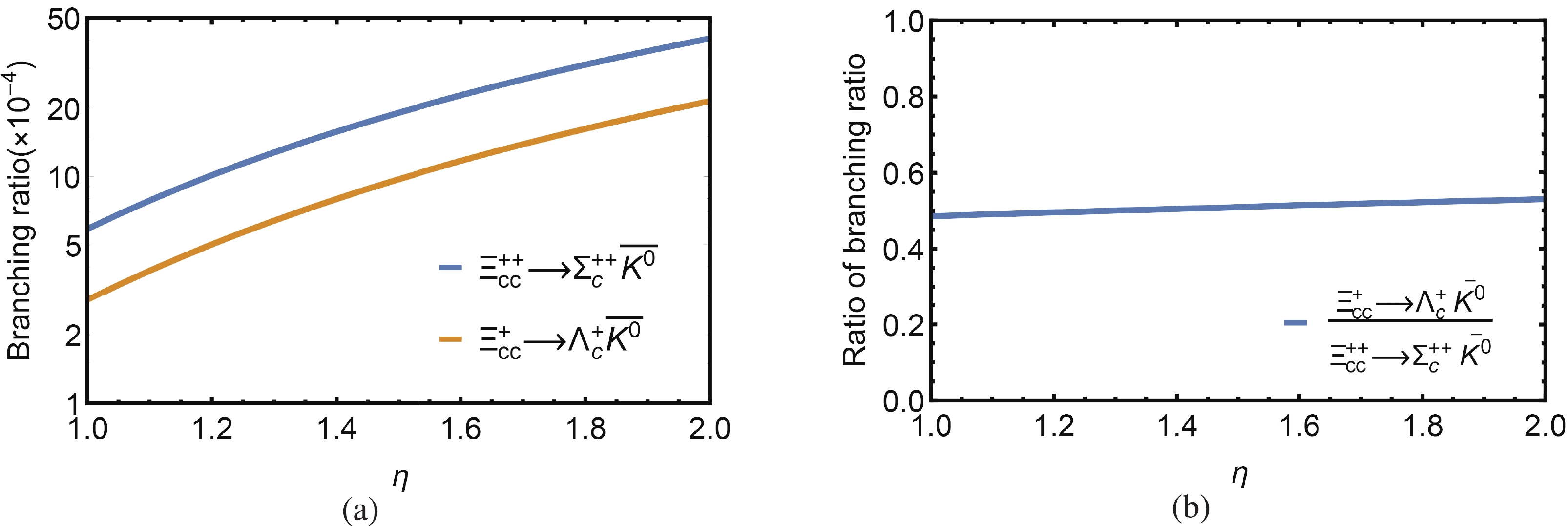
Figure 4. (color online) (a) Theoretical predictions for the branching ratios of
$\Xi_{cc}^{++}\to\Sigma_c^{++}\overline{K}^{0}$ and$\Xi_{cc}^{+}\to\Lambda_c^+\overline{K}^{0}$ in logarithmic coordinates; (b) ratio of branching fractions with$\eta$ varying from 1.0 to 2.0.The problem of large uncertainty induced by varying the value of
$ \eta $ can be solved by the ratio of branching fractions, first proposed in Ref. [16]. From Fig. 4(a), we can easily find that the dependences of the branching ratios of$ \Xi_{cc}^{++} \to \Sigma_c^{++} \overline{K}^0 $ and$ \Xi_{cc}^+ \to \Lambda_c^+ \overline{K}^0 $ on$ \eta $ have similar line shapes. That means that the dependence of the ratio of the two branching fractions on$ \eta $ can be mostly canceled. Therefore, the ratio of branching fractions will be insensitive to the value of$ \eta $ , as Fig. 4(b) shows. From Fig. 4(a), the branching fraction of$ \Xi_{cc}^{++}\to \Sigma_c^{++}\overline K^0 $ changes from$ 0.59\times 10^{-3} $ to$ 4.06\times 10^{-3} $ with the parameter$ \eta $ varying from 1.0 to 2.0. Similarly, for$ \Xi_{cc}^{+}\to \Lambda_c^{+}\overline K^0 $ , it changes from$ 0.29\times 10^{-3} $ to$ 2.15\times 10^{-3} $ . The branching fractions of both processes vary by nearly one order of magnitude. Taking the central values of the above results, they are$ (2.33\pm1.74)\times10^{-3} $ and$ (1.22\pm0.93)\times10^{-3} $ , respectively, with the uncertainties around 75%. However, the ratio of the above branching fractions is$ 0.48\sim 0.53 $ , seen in Fig. 4(b). Written as$ 0.51\pm0.03 $ , the uncertainty of the ratio is 5%. Therefore, almost 70% of the uncertainties of the absolute branching fractions are cancelled by the ratio of branching fractions. Similar cancelation behavior also happens between all other decay channels. The reason for this cancelation is as follows. The difference in $\eta$ of the triangle diagrams for the two modes of$ \Xi_{cc}^{++} \to \Sigma_c^{++} \overline{K}^0 $ and$ \Xi_{cc}^+ \to \Lambda_c^+ \overline{K}^0 $ mainly stems from the strong coupling constants and the masses of the particles in the rescattering diagrams. The corresponding quantities for different decay modes can be related under the flavor$ SU(3) $ symmetry. The dependence on$ \eta $ should be similar for both these modes, and can thus be mostly cancelled in the ratio of branching fractions. In this way, the theoretical uncertainties can be brought under control. That is why we could successfully predict the discovery channels of$ \Xi_{cc}^{++} $ in Ref. [16]. In this work, we will present the results of branching fractions with different values of$ \eta $ , to show the absolute uncertainty of any individual mode. The reader can take a ratio between any two processes to get a more reliable result.Note that the above cancellation can be broken down by the so-called triangle singularity, in which all the intermediate particles are on-shell. We will not tackle this issue in this work. Besides, as discussed in Ref. [58], the values of
$ \eta $ are not identical for different classes of decay modes. For example, the values of$ \eta $ are different for$ B\to D\pi $ and$ B\to \pi\pi $ decays, to satisfy the constraints from the experimental data. This can be easily understood in that the exchanged particles are different in different decay modes. Therefore, we should be careful to consider the values of$ \eta $ for different classes of decay processes. -
We list all the branching ratios of the decay modes
$ {\cal{B}}_{cc}\to{\cal{B}}_cP $ in Tables 2-5. The short-distance dynamics dominant channels (with T topology) are presented in Table 2. For the long-distance-dominated processes, the numerical results are classified into three groups according to the CKM matrix elements: (a) the Cabibbo-favored (CF) decays induced by$ c\to su\bar{d} $ (with the CKM element$ V_{cs}^\ast V_{ud} $ ) are listed in Table 3; (b) the singly Cabibbo-suppressed (SCS) decays induced by$ c\to du\bar{d} $ or$ c\to su\bar{s} $ (with the CKM element$ V_{cd}^\ast V_{ud} $ or$ V_{cs}^\ast V_{us} $ ) are listed in Table 4; and (c) the doubly Cabibbo-suppressed (DCS) decays induced by$ c\to du\bar{s} $ (with the CKM element$ V_{cd}^\ast V_{us} $ ) are given in Table 5. The topological amplitudes for the channels with the sextet single charmed baryons are distinguished from the anti-triplet baryons by adding a$ tilde $ , e.g.$ \tilde{T} $ .Particle Decay mode Topology $ {\cal{BR}}_{T_{SD}} $ (%)

$ {\cal{BR}}_{\eta=1.0} $ (%)

$ {\cal{BR}}_{\eta=1.5} $ (%)

$ {\cal{BR}}_{\eta=2.0} $ (%)

CKM $ \Xi_{cc}^{++} $ 

$ \to\Xi_c^+\pi^+ $ 

$ \lambda_{sd} (T+C^{\prime}) $ 

6.76 7.11 8.48 10.75 CF $ \to\Xi_c^{\prime +}\pi^+ $ 

$ {{1}/{\sqrt{2}}}\lambda_{sd}\big(\tilde{T}+\tilde{C}^{\prime}\big) $ 

4.71 4.72 4.72 4.74 CF $ \to\Sigma_c^+\pi^+ $ 

$ {{1}/{\sqrt{2}}}\lambda_{d}\big(\tilde{T}+\tilde{C}^{\prime}\big) $ 

0.248 0.251 0.255 0.261 SCS $ \to\Lambda_c^+\pi^+ $ 

$ \lambda_d(T+C^{\prime}) $ 

0.386 0.390 0.393 0.396 SCS $ \to\Xi_c^{\prime +}K^+ $ 

$ {{1}/{\sqrt{2}}}\lambda_s \big(\tilde{T}+\tilde{C}^{\prime}\big) $ 

0.303 0.304 0.304 0.305 SCS $ \to\Xi_c^+K^+ $ 

$ \lambda_s(T+C^{\prime}) $ 

0.538 0.538 0.538 0.538 SCS $ \to\Lambda_c^+K^+ $ 

$ \lambda_{ds}(T+C^{\prime}) $ 

0.028 0.029 0.030 0.031 DCS $ \to\Sigma_c^+K^+ $ 

$ {{1}/{\sqrt{2}}}\lambda_{ds}\big(\tilde{T}+ \tilde{C}^{\prime}\big) $ 

0.016 0.016 0.018 0.021 DCS
$ \Xi_{cc}^{+} $ 

$ \to\Xi_c^0\pi^+ $ 

$ \lambda_{sd}(T-E_2) $ 

4.08 4.34 4.58 4.74 CF $ \to\Xi_c^{\prime 0}\pi^+ $ 

$ {{1}/{\sqrt{2}}} \lambda_{sd} \big(\tilde{T}+\tilde{E}_2\big) $ 

2.84 2.84 2.84 2.84 CF $ \to\Sigma_c^0\pi^+ $ 

$ \lambda_d(\tilde{T}+\tilde{E}_2) $ 

0.31 0.32 0.33 0.35 SCS $ \to\Xi_c^{\prime 0}K^+ $ 

$ {{1}/{\sqrt{2}}}\big(\lambda_s \tilde{T} + \lambda_d \tilde{E}_2\big) $ 

0.18 0.18 0.18 0.18 SCS $ \to\Xi_c^{0}K^+ $ 

$ \lambda_s T + \lambda_d E_2 $ 

0.32 0.32 0.33 0.33 SCS $ \to\Sigma_c^0K^+ $ 

$ \lambda_{ds}\tilde{T} $ 

0.02 DCS
$ \Omega_{cc}^{+} $ 

$ \to\Omega_c^{0}\pi^+ $ 

$ \lambda_{sd}\tilde{T} $ 

6.09 CF $ \to\Xi_c^{0}\pi^+ $ 

$ -\lambda_d T - \lambda_s E_2 $ 

0.23 0.23 0.23 0.23 SCS $ \to\Xi_c^{\prime 0}\pi^+ $ 

$ {{1}/{\sqrt{2}}}\big(\lambda_d \tilde{T} + \lambda_s \tilde{E}_2\big) $ 

0.16 0.16 0.17 0.17 SCS $ \to\Omega_c^{0}K^+ $ 

$ \lambda_s\big(\tilde{T}+\tilde{E}_2\big) $ 

0.38 0.40 0.40 0.40 SCS $ \to\Xi_c^0K^+ $ 

$ \lambda_{ds}(-T+E_2) $ 

0.019 0.091 0.091 0.091 DCS $ \to\Xi_c^{\prime 0}K^+ $ 

$ {{1}/{\sqrt{2}}}\lambda_{ds} \big(\tilde{T}+\tilde{E}_2\big) $ 

0.011 0.011 0.011 0.011 DCS Table 2. Branching ratios for the short-distance dynamics dominated modes. "CF", "SCS" and "DCS" represent CKM favored, singly CKM suppressed and doubly CKM suppressed processes, respectively.
Particles Decay modes Topology $ {\cal{BR}}_{T_{SD}}(\times 10^{-6}) $ 

$ {\cal{BR}}_{\eta=1.0}(\times 10^{-6}) $ 

$ {\cal{BR}}_{\eta=1.5}(\times 10^{-6}) $ 

$ {\cal{BR}}_{\eta=2.0}(\times 10^{-6}) $ 

$ \Xi_{cc}^{++} $ 

$ \to\Sigma_c^{++}K^0 $ 

$ \tilde{C} $ 

0.043 1.31 4.69 10.75
$ \Xi_{cc}^{+} $ 

$ \to\Sigma_c^+K^0 $ 

$ {{1}/{\sqrt{2}}}\big(\tilde{C} + \tilde{C}^{\prime}\big) $ 

0.035 4.52 16.0 36.4 $ \to\Lambda_c^+K^0 $ 

$ -C+C^{\prime} $ 

0.05 2.39 8.88 21.0
$ \Omega_{cc}^{+} $ 

$ \to\Sigma_c^+\pi^0 $ 

$ {{1}/{2}}(-\tilde{E}_1+\tilde{E}_2) $ 

0.07 0.23 0.52 $ \to\Sigma_c^+\eta_1 $ 

$ {{1}/{\sqrt{6}}}\big(\tilde{C}^{\prime}+\tilde{E}_1+\tilde{E}_2\big) $ 

0.14 0.45 0.89 $ \to\Sigma_c^+\eta_8 $ 

$ {{1}/{2\sqrt{3}}}\big(-2\tilde{C}^{\prime}+\tilde{E}_1+\tilde{E}_2\big) $ 

0.09 0.30 0.66 $ \to\Lambda_c^+\pi^0 $ 

$ -{{1}/{\sqrt{2}}}(E_1+E_2) $ 

0.19 0.61 1.34 $ \to\Lambda_c^+\eta_1 $ 

$ {{1}/{\sqrt{3}}}(C^{\prime}+E_1-E_2) $ 

0.59 1.89 4.13 $ \to\Lambda_c^+\eta_8 $ 

$ -{{1}/{\sqrt{6}}}(2C^{\prime}-E_1+E_2) $ 

0.28 0.89 1.97 $ \to\Sigma_c^0\pi^+ $ 

$ \tilde{E}_2 $ 

0.14 0.45 0.91 $ \to\Sigma_c^{++}\pi^- $ 

$ \tilde{E}_1 $ 

0.16 0.59 1.31 $ \to\Xi_c^{\prime +}K^0 $ 

$ {{1}/{\sqrt{2}}}\big(\tilde{C}+\tilde{E}_1\big) $ 

0.028 9.68 31.9 68.0 $ \to\Xi_c^+K^0 $ 

$ -C+E_1 $ 

0.045 0.82 2.84 6.54 Table 5. Same as Table 3 but for the long-distance-dominated doubly Cabibbo-suppressed modes.
Particles Decay modes Topology $ {\cal{BR}}_{T_{SD}}(\times 10^{-3}) $ 

$ {\cal{BR}}_{\eta=1.0}(\times 10^{-3}) $ 

$ {\cal{BR}}_{\eta=1.5}(\times 10^{-3}) $ 

$ {\cal{BR}}_{\eta=2.0}(\times 10^{-3}) $ 

$ \Xi_{cc}^{++} $ 

$ \to\Sigma_c^{++}\overline{K}^0 $ 

$ \tilde{C} $ 

0.015 0.59 1.91 4.06
$ \Xi_{cc}^{+} $ 

$ \to\Omega_c^0K^+ $ 

$ \tilde{E}_2 $ 

0.049 0.15 0.29 $ \to\Sigma_c^+\overline{K}^0 $ 

$ {{1}/{\sqrt{2}}}\big(\tilde{C}+\tilde{E}_1\big) $ 

0.009 1.55 4.72 9.95 $ \to\Lambda_c^+\overline{K}^0 $ 

$ -C+E_1 $ 

0.017 0.29 0.98 2.15 $ \to\Sigma_c^{++}K^- $ 

$ \tilde{E}_1 $ 

0.075 0.26 0.55 $ \to\Xi_c^{\prime +}\pi^0 $ 

$ {{1}/{2}}(-\tilde{C}^{\prime}+\tilde{E}_2) $ 

0.33 0.98 1.97 $ \to\Xi_c^{\prime +}\eta_1 $ 

$ {{1}/{\sqrt{6}}}(\tilde{C}^{\prime}+\tilde{E}_1+\tilde{E}_2) $ 

0.57 1.73 3.50 $ \to\Xi_c^{\prime +}\eta_8 $ 

$ {{1}/{2\sqrt{3}}}(\tilde{C}^{\prime}-2\tilde{E}_1+\tilde{E}_2) $ 

0.22 0.66 1.37 $ \to\Xi_c^+\pi^0 $ 

$ -{{1}/{\sqrt{2}}}(C^{\prime}+E_2) $ 

3.24 10.2 21.0 $ \to\Xi_c^+\eta_1 $ 

$ {{1}/{\sqrt{3}}}(C^{\prime}+E_1-E_2) $ 

0.18 0.57 1.20 $ \to\Xi_c^+\eta_8 $ 

$ {{1}/{\sqrt{6}}}(C^{\prime}-2E_1-E_2) $ 

0.11 0.35 0.66
$ \Omega_{cc}^{+} $ 

$ \to\Xi_c^{\prime +}\overline{K}^0 $ 

$ {{1}/{\sqrt{2}}}(\tilde{C}+\tilde{C}^{\prime}) $ 

0.010 1.10 3.38 6.84 $ \to\Xi_c^+\overline{K}^0 $ 

$ -C+C^{\prime} $ 

0.017 0.73 2.30 4.38 Table 3. Branching ratios for the long-distance-dominated Cabibbo-favored (
$ \lambda_{sd} $ ) modes. For the channels involving internalW-emission contributions, the short-distance factorizable contributions are also listed in the fourth column, for comparison. Particles Decay modes Topology $ {\cal{BR}}_{T_{SD}}(\times 10^{-5}) $ 

$ {\cal{BR}}_{\eta=1.0}(\times 10^{-5}) $ 

$ {\cal{BR}}_{\eta=1.5}(\times 10^{-5}) $ 

$ {\cal{BR}}_{\eta=2.0}(\times 10^{-5}) $ 

$ \Xi_{cc}^{++} $ 

$ \to\Sigma_c^{++}\pi^0 $ 

$ -{{1}/{\sqrt{2}}}\tilde{C} $ 

0.062 3.39 11.5 25.4 $ \to\Sigma_c^{++}\eta_1 $ 

$ {{1}/{\sqrt{3}}}(\lambda_d+\lambda_s) \tilde{C} $ 

0.022 1.18 2.43 4.35 $ \to\Sigma_c^{++}\eta_8 $ 

$ {{1}/{\sqrt{6}}}(\lambda_d-2\lambda_s) \tilde{C} $ 

0.059 3.24 8.62 15.3
$ \Xi_{cc}^{+} $ 

$ \to\Sigma_c^{+}\pi^0 $ 

$ {{1}/{2}}\lambda_d\big(-\tilde{C}-\tilde{C}^{\prime}+\tilde{E}_1+\tilde{E}_2\big) $ 

0.038 3.85 12.1 25.0 $ \to\Sigma_c^{+}\eta_1 $ 

$ {{1}/{\sqrt{6}}}\big[\lambda_d\big(\tilde{C}+\tilde{C}^{\prime}+\tilde{E}_1+\tilde{E}_2\big) + \lambda_s\tilde{C}\big] $ 

0.026 2.52 7.69 16.4 $ \to\Sigma_c^{+}\eta_8 $ 

$ {{1}/{2\sqrt{3}}}\big[\lambda_d\big(\tilde{C}+\tilde{C}^{\prime}+\tilde{E}_1+\tilde{E}_2\big) - 2\lambda_s\tilde{C}\big] $ 

0.016 1.64 4.52 8.70 $ \to\Lambda_c^{+}\pi^0 $ 

$ {{1}/{\sqrt{2}}}\lambda_d(C-C^{\prime}-E_1-E_2) $ 

0.057 1.53 4.76 9.79 $ \to\Lambda_c^{+}\eta_1 $ 

$ {{1}/{\sqrt{3}}}\big[\lambda_d\big(C^{\prime}-C+E_1-E_2\big) - \lambda_sC\big] $ 

0.031 0.84 1.90 4.07 $ \to\Lambda_c^{+}\eta_8 $ 

$ {{1}/{\sqrt{6}}}\big[\lambda_d\big(C^{\prime}-C+E_1-E_2\big) + 2\lambda_sC\big] $ 

0.020 0.55 0.93 1.59 $ \to\Sigma_c^{++}\pi^- $ 

$ \lambda_d \tilde{E}_1 $ 

0.38 1.18 2.46 $ \to\Xi_c^{\prime +}K^0 $ 

$ {{1}/{\sqrt{2}}} \big(\lambda_s\tilde{C}^{\prime}+\lambda_d\tilde{E}_1\big) $ 

1.17 3.79 8.00 $ \to\Xi_c^+K^0 $ 

$ \lambda_sC^{\prime}+\lambda_dE_1 $ 

2.77 8.75 18.1
$ \Omega_{cc}^{+} $ 

$ \to\Sigma_c^+\overline{K}^0 $ 

$ {{1}/{\sqrt{2}}}\big(\lambda_d \tilde{C}^{\prime} + \lambda_s \tilde{E}_1\big) $ 

0.26 0.75 1.48 $ \to\Lambda_c^+\overline{K}^0 $ 

$ \lambda_dC^{\prime}+\lambda_sE_1 $ 

0.52 1.66 3.49 $ \to\Sigma_c^{++}K^- $ 

$ \lambda_s \tilde{E}_1 $ 

0.23 0.77 1.69 $ \to\Xi_c^{\prime +}\pi^0 $ 

$ {{1}/{2}}\big(-\lambda_d \tilde{C} + \lambda_s \tilde{E}_2\big) $ 

0.38 1.48 3.61 $ \to\Xi_c^{\prime +}\eta_1 $ 

$ {{1}/{\sqrt{6}}}\big[\lambda_s\big(\tilde{C}+\tilde{C}^{\prime}+\tilde{E}_1+\tilde{E}_2\big) + \lambda_d\tilde{C}\big] $ 

0.49 1.71 3.45 $ \to\Xi_c^{\prime +}\eta_8 $ 

$ {{1}/{2\sqrt{3}}}\big[\lambda_s\big(\tilde{E}_2-2\tilde{C}-2\tilde{C}^{\prime}-2\tilde{E}_1\big) +\lambda_d\tilde{C}\big] $ 

2.04 6.26 13.0 $ \to\Xi_c^+\pi^0 $ 

$ {{1}/{\sqrt{2}}}(\lambda_dC-\lambda_sE_2) $ 

4.50 13.2 26.0 $ \to\Xi_c^+\eta_1 $ 

$ {{1}/{\sqrt{3}}}\big[\lambda_s\big(C^{\prime}-C+E_1-E_2\big) - \lambda_dC\big] $ 

11.3 37.3 77.3 $ \to\Xi_c^+\eta_8 $ 

$ {{1}/{\sqrt{6}}}\big[\lambda_s\big(2C-2C^{\prime}+2E_1-E_2\big) -\lambda_dC\big] $ 

6.66 21.9 45.5 Table 4. Same as Table 3 but for the long-distance-dominated singly Cabibbo-suppressed modes.
In Table 2, it is clear that the factorizable short-distance contributions of diagram amplitude T are dominant relative to the long-distance contributions of
$ C^{\prime} $ and$ E_2 $ . When the parameter$ \eta $ tends to$ 2.0 $ , the long-distance contributions of$ C^{\prime} $ and$ E_2 $ also have a visible or comparable effect. On the other hand, from Tables 3-5, the long-distance dynamics dominates the decay modes in Table 3 to 5, since the only calculable short-distance amplitude$ C_{SD} $ is heavily suppressed by the effective Wilson coefficient$ a_2(\mu) $ at the charm mass scale, i.e.$ a_2(m_c) = -0.017 $ is much smaller than$ a_1(m_c) = 1.07 $ . The latter is used at the weak decay vertex of the triangle diagram in our calculations. -
The topological diagrams have the relations of
$ {\dfrac{|C|}{ |T|}}\sim{\dfrac{|C^{\prime}|}{ |C|}}\sim{\dfrac{|E_1|}{ |C|}}\sim{\dfrac{|E_2|}{ |C|}}\sim O\left({\dfrac{\Lambda^h_{\rm{QCD}}}{ m_Q}}\right) $ in heavy baryon decays, manifested by the soft-collinear effective theory [64, 65]. These relations are important in phenomenological studies on the searches for double-heavy-flavor baryons, and give us more hints on the dynamics of heavy baryon decays. From the above relations, all the tree-level topological diagrams are at the same order in charmed baryon decays, due to$ \Lambda^h_{\rm{QCD}}/ m_c\sim1 $ . It would be very useful to numerically test these relations in our framework.From the amplitudes of
$ \Xi_{cc}^{++}\to \Sigma_c^{++}\overline{K}^{0} $ $\big( \tilde{C} \big)$ and$ \Xi_{cc}^{++}\to \Xi_c^{\prime +}\pi^+ $ $\big( {1/\sqrt{2}}\big(\tilde{T}+\tilde{C}^{\prime}\big) \big)$ , we obtain the ratios$ \tilde{C}_{LD}/\tilde{T}_{SD} $ and$ \tilde{C}^{\prime}_{LD}/\tilde{C}_{LD} $ :$ \frac{|\tilde{C}_{LD}|}{|\tilde{T}_{SD}|} = \frac{|{\cal{A}}(\Xi_{cc}^{++}\to \Sigma_c^{++}\overline{K}^{0})|_{LD}}{\sqrt{2}|{\cal{A}}(\Xi_{cc}^{++}\to \Xi_c^{\prime +}\pi^+)|_{SD}} = 0.21\sim 0.55, $

(26) $ \frac{|\tilde{C}^{\prime}_{LD}|}{|\tilde{C}_{LD}|} = \frac{\sqrt{2}|{\cal{A}}(\Xi_{cc}^{++}\to \Xi_c^{\prime +}\pi^+)|_{LD}}{|{\cal{A}}(\Xi_{cc}^{++}\to \Sigma_c^{++}\overline{K}^{0})|_{LD}} = 1.33\sim 1.45. $

(27) The ratio
$ \tilde{C}^{\prime}_{LD}/\tilde{C}_{LD} $ can also be calculated by the decay channels$ \Xi_{cc}^{++} \to \Sigma_c^{++}\pi^0 $ $\big( -{1/\sqrt{2}}\tilde{C} \big)$ ,$ \Xi_{cc}^{++} \to \Sigma_c^+\pi^+ $ $\big( {1/\sqrt{2}}\big(\tilde{T}+\tilde{C}^{\prime}\big) \big)$ ,$ \Xi_{cc}^{++} \to \Xi_c^{\prime +}K^+ $ $\big( {1/\sqrt{2}}\big(\tilde{T}+\tilde{C}^{\prime}\big) \big)$ and$ \Xi_{cc}^{++}\to $ $ \Sigma_c^{++}K^0 $ $\big( \tilde{C} \big)$ ,$ \Xi_{cc}^{++}\to\Sigma_c^+K^+ $ $\big( {1/\sqrt{2}}\big(\tilde{T}+\tilde{C}^{\prime}\big) \big)$ as:$ \frac{|\tilde{C}^{\prime}_{LD}|}{|\tilde{C}_{LD}|} = \frac{|{\cal{A}}(\Xi_{cc}^{++}\to\Sigma_c^+\pi^+)|_{LD}}{|{\cal{A}}(\Xi_{cc}^{++}\to\Sigma_c^{++}\pi^0)|_{LD}} = 0.72\sim 0.88, $

(28) $ \frac{|\tilde{C}^{\prime}_{LD}|}{|\tilde{C}_{LD}|} = \frac{|{\cal{A}}(\Xi_{cc}^{++}\to\Xi_c^{\prime+}K^+)|_{LD}}{|{\cal{A}}(\Xi_{cc}^{++}\to\Sigma_c^{++}\pi^0)|_{LD}} = 0.69\sim 0.85, $

(29) $ \frac{|\tilde{C}^{\prime}_{LD}|}{|\tilde{C}_{LD}|}= \frac{\sqrt{2}|{\cal{A}}(\Xi_{cc}^{++}\to\Sigma_c^+K^+)|_{LD}}{|{\cal{A}}(\Xi_{cc}^{++}\to\Sigma_c^{++}K^0)|_{LD}} = 0.98\sim 1.24. $

(30) In the following, to consider the relations between C,
$ E_1 $ and$ E_2 $ , it would be more convenient to study the processes with a pure topological diagram. The advantage of avoiding interference between diagrams is that they could be directly determined by experimental data in the future.In Table 3, by the three single amplitude channels
$ \Xi_{cc}^{+}\to\Sigma_c^{++}K^- $ $\big( \tilde{E}_1 \big)$ ,$ \Xi_{cc}^{+} \to\Omega_c^0K^+ $ $\big( \tilde{E}_2 \big)$ and$ \Xi_{cc}^{++}\to\Sigma_c^{++}\overline{K}^{0} $ $\big( \tilde{C} \big)$ , the ratios among the amplitudes$ \tilde{E}_{1LD} $ ,$ \tilde{E}_{2LD} $ and$ \tilde{C}_{LD} $ can easily be calculated, giving:$ \frac{|\tilde{E}_{1LD}|}{|\tilde{C}_{LD}|} = \frac{|{\cal{A}}(\Xi_{cc}^+\to\Sigma_c^{++}K^-)|_{LD}}{|{\cal{A}}(\Xi_{cc}^{++}\to\Sigma_c^{++}\overline{K}^{0})|_{LD}} = 0.45\sim 0.46, $

(31) $ \frac{|\tilde{E}_{2LD}|}{|\tilde{C}_{LD}|} = \frac{|{\cal{A}}(\Xi_{cc}^+\to\Omega_c^0K^+)|_{LD}}{|{\cal{A}}(\Xi_{cc}^{++}\to\Sigma_c^{++}\overline{K}^{0})|_{LD}} = 0.38\sim 0.40, $

(32) $ \frac{|\tilde{E}_{1LD}|}{|\tilde{E}_{2LD}|} = \frac{|{\cal{A}}(\Xi_{cc}^+\to\Sigma_c^{++}K^-)|_{LD}}{|{\cal{A}}(\Xi_{cc}^+\to\Omega_c^0K^+)|_{LD}} = 1.12\sim 1.24. $

(33) From above, the ratios
$ \tilde{E}_{1LD}/\tilde{C}_{SD} $ and$ \tilde{E}_{2LD}/\tilde{C}_{SD} $ have similar values, at first order. The ratios between$ \tilde{E}_{1LD} $ and$ \tilde{C}_{SD} $ can also be calculated from Table 4, i.e. from the modes$ \Xi_{cc}^{++}\to\Sigma_c^{++}\pi^0 $ $\big( -{1}/{\sqrt{2}}\tilde{C} \big)$ ,$ \Xi_{cc}^{+}\to $ $ \Sigma_c^{++}\pi^- $ $\big( \tilde{E}_1 \big)$ and$ \Omega_{cc}^{+}\to\Sigma_c^{++}K^- $ $\big( \tilde{E}_1 \big)$ :$ \frac{|\tilde{E}_{1LD}|}{|\tilde{C}_{LD}|} = \frac{|{\cal{A}}(\Xi_{cc}^+\to\Sigma_c^{++}\pi^-)|_{LD}}{\sqrt{2}|{\cal{A}}(\Xi_{cc}^{++}\to\Sigma_c^{++}\pi^0)|_{LD}} = 0.28\sim 0.26, $

(34) $ \frac{|\tilde{E}_{1LD}|}{|\tilde{C}_{LD}|} = \frac{|{\cal{A}}(\Omega_{cc}^+\to\Sigma_c^{++}K^-)|_{LD}}{\sqrt{2}|{\cal{A}}(\Xi_{cc}^{++}\to\Sigma_c^{++}\pi^0)|_{LD}} = 0.29\sim 0.30. $

(35) We can verify the results using the data from Table 5. By the three channels
$ \Xi_{cc}^{++}\to\Sigma_c^{++}K^0 $ $\big( \tilde{C} \big)$ ,$ \Omega_{cc}^{+}\to\Sigma_c^0\pi^+ $ $\big( \tilde{E}_2 \big)$ and$ \Omega_{cc}^{+}\to\Sigma_c^{++}\pi^- $ $\big( \tilde{E}_1 \big)$ , we get the ratios as:$ \frac{|\tilde{E}_{2LD}|}{|\tilde{C}_{LD}|} = \frac{|{\cal{A}}(\Omega_{cc}^+\to\Sigma_c^0\pi^+)|_{LD}}{|{\cal{A}}(\Xi_{cc}^{++}\to\Sigma_c^{++}K^0)|_{LD}} = 0.34\sim 0.37, $

(36) $ \frac{|\tilde{E}_{1LD}|}{|\tilde{C}_{LD}|} = \frac{|{\cal{A}}(\Omega_{cc}^+\to\Sigma_c^{++}\pi^-)|_{LD}}{|{\cal{A}}(\Xi_{cc}^{++}\to\Sigma_c^{++}K^0)|_{LD}} = 0.40\sim 0.41.$

(37) From Eqs. (26-37), considering the relatively large parameter uncertainty, all these results are consistent with the relations found in [64, 65],
$ \frac{|C|}{|T|}\sim\frac{|C^{\prime}|}{|C|}\sim\frac{|E_1|}{|C|}\sim\frac{|E_2|}{|C|}\sim {\cal{O}}\left({\Lambda^h_{\rm QCD}\over m_c}\right)\sim {\cal{O}}(1). $

(38) Some results in Eqs. (26-37) are different from each other. This can be understood by the flavor
$ SU(3) $ breaking effects, shown in the following subsection.As mentioned in Sec. II A, the long-distance quark-loop diagrams are also taken into account in our calculations. Taking
$ \Xi_{cc}^+\to\Sigma_c^{++}\pi^- $ as an example, the quark-loop topological diagrams and the corresponding hadronic triangle diagrams are shown in Fig. 5. It can be expected that any individual loop diagram is as large as the tree diagrams. However, the d-quark and s-quark loop diagrams are mostly cancelled due to the GIM mechanism. Therefore, the total contribution of quark loop diagrams comes from the flavor$ SU(3) $ symmetry breaking effects. Numerically, the magnitudes of the d-quark loop, s-quark loop and the sum of the both loop diagrams are$ |{\cal{A}}_{d}| = 2.6\times 10^{-7} $ GeV,$ |{\cal{A}}_{s}| = 1.0\times 10^{-7} $ GeV,$ |{\cal{A}}_{d+s}| = $ $ 1.5\times 10^{-7} $ GeV, respectively. It can be seen that the long-distance dynamics contributes the relatively large$ SU(3) $ breaking effect. It is difficult to test this effect in the doubly charmed baryons in experiments. We will investigate the long-distance quark-loop contributions in the D meson and$ \Lambda_c $ decays in a future study.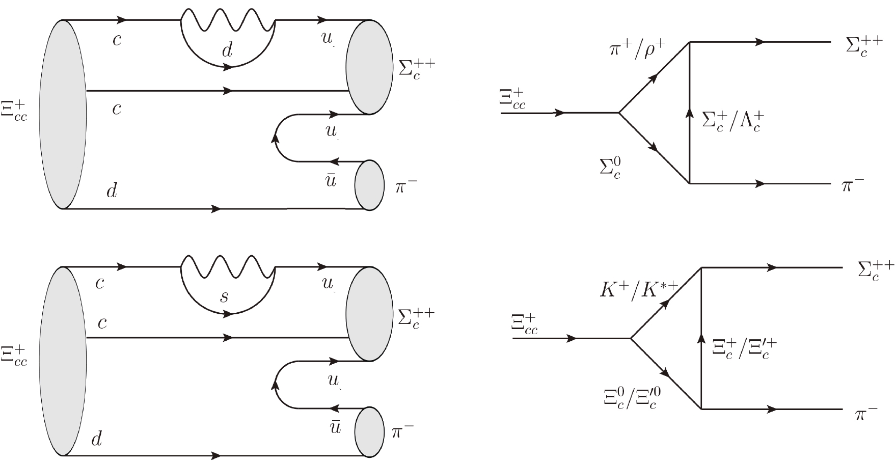
Figure 5. Quark-loop topological diagrams and their corresponding hadronic triangle diagrams for
$\Xi_{cc}^+\to\Sigma_c^{++}\pi^-$ . -
Flavor
$ SU(3) $ symmetry is very significant in the weak decays of heavy hadrons. In terms of a few SU(3) irreducible amplitudes, a number of relations between the widths of doubly charmed baryon decays are obtained [73]. It is important to numerically test the flavor$ SU(3) $ symmetry and its breaking effects.In the following, we show our numerical results for the ratios of decay widths. In the
$ SU(3) $ limit, they should be unity. Any deviation would indicate$ SU(3) $ breaking effects.$ \Gamma\big( \Xi_{cc}^{++}\to\Lambda_c^+\pi^+ \big)/\Gamma\big( \Xi_{cc}^{++}\to\Xi_c^+K^+ \big) = |\lambda_d(T+C^{\prime})|^2/|\lambda_s(T+C^{\prime})|^2= 0.73\sim 0.74, $ 
(39) $ \Gamma\big( \Xi_{cc}^+\to\Xi_c^+K^0\big) / \Gamma\big( \Omega_{cc}^+\to\Lambda_c^+\overline{K}^0 \big)\ \ = |\lambda_s C^{\prime}+\lambda_d E_1|^2/|\lambda_d C^{\prime}+\lambda_s E_1|^2 = 6.67\sim 6.85, $

(40) $ \Gamma\big( \Omega_{cc}^+\to\Xi_c^0\pi^+ \big)/ \Gamma\big( \Xi_{cc}^+\to\Xi_c^0K^+ \big)\ \ = |-\lambda_d T-\lambda_s E_2 |^2/| \lambda_s T+\lambda_d E_2|^2= 0.54\sim 0.56, $

(41) $ \Gamma\big( \Xi_{cc}^{++}\to\Sigma_c^{++}\pi^0 \big)/\frac{1}{3}\Gamma\big( \Xi_{cc}^{++}\to\Sigma_c^{++}\eta_8 \big) = |-\frac{1}{\sqrt{2}}\tilde{C} |^2/|-\frac{1}{\sqrt{6}}(\lambda_d-2\lambda_s)\tilde{C} |^2= 3.14\sim 4.98, $

(42) $ \Gamma\big( \Xi_{cc}^{++}\to\Sigma_c^+\pi^+ \big)/ \Gamma\big( \Xi_{cc}^{++}\to\Xi_c^{\prime+}K^+ \big)\ \ = | \frac{1}{\sqrt{2}}\lambda_d(\tilde{T}+\tilde{C}^{\prime})|^2/| \frac{1}{\sqrt{2}}\lambda_s(\tilde{T}+\tilde{C}^{\prime})|^2 = 1.28\sim 1.30, $

(43) $ \Gamma\big( \Xi_{cc}^+\to\Sigma_c^{++}\pi^- \big)/\Gamma\big( \Omega_{cc}^+\to\Sigma_c^{++}K^- \big)\ \ = |\lambda_d \tilde{E}_1|^2/|\lambda_s \tilde{E}_1 |^2 = 1.87\sim 2.12, $

(44) $ \Gamma\big( \Xi_{cc}^+\to\Sigma_c^{0}\pi^+ \big) / \Gamma\big( \Omega_{cc}^+\to\Omega_c^{0}K^+ \big)\ = | \lambda_d(\tilde{T}+\tilde{E}_2)|^2/|\lambda_s(\tilde{T}+\tilde{E}_2) |^2 = 1.03\sim 1.13, $

(45) $ \Gamma\big( \Xi_{cc}^+\to\Xi_c^{\prime+}K^0 \big)/\Gamma\big( \Omega_{cc}^+\to\Sigma_c^+\overline{K}^0 \big)\ = | \frac{1}{\sqrt{2}}(\lambda_s\tilde{C}^{\prime}+\lambda_d\tilde{E}_1)|^2/|\frac{1}{\sqrt{2}}(\lambda_d\tilde{C}^{\prime}+\lambda_s\tilde{E}_1) |^2= 5.79\sim 6.95,$

(46) $ \Gamma\big( \Omega_{cc}^+\to\Xi_c^{\prime 0}\pi^+ \big)/ \Gamma\big( \Xi_{cc}^+\to\Xi_c^{\prime 0}K^+ \big)\ = | \frac{1}{\sqrt{2}}(\lambda_d\tilde{T}^{\prime}+\lambda_s\tilde{E}_2|^2/|\frac{1}{\sqrt{2}}(\lambda_s\tilde{T}^{\prime}+\lambda_d\tilde{E}_2) |^2 = 0.69\sim 0.74. $

(47) From the above numerical results, it can be found that the long-distance final-state interactions can contribute to the large
$ SU(3) $ breaking effect. It stems from the exchanged particles, hadronic strong coupling constants, transition form factors, decay constants, and interference between different diagrams. In our calculation of Eq. (40) and Eq. (46), the large values mainly stem from the strong coupling constants. Taking$ \Gamma\big( \Xi_{cc}^{+}\to\Xi_c^+K^0\big) / $ $ \Gamma\big( \Omega_{cc}^{+}\to\Lambda_c^+\overline{K}^0 \big) = 6.67\sim 6.85 $ as an example, a factor of 2.5 in the amplitude could account for the large ratio. The decay mode$ \Xi_{cc}^{+}\to\Xi_c^+K^0 $ is dominated by the triangle diagram$ {\cal{M}}(K^+,\Xi_c^0;\rho^+) $ , while$ \Omega_{cc}^{+}\to\Lambda_c^+\overline{K}^0 $ is dominated by$ {\cal{M}}(\pi^+,\Xi_c^0;K^{\ast +}) $ . To evaluate these two triangle diagrams, we need strong coupling constants$ f_1(\Xi_c^+\to\Xi_c^0\rho^+) = 8.5 $ ,$ f_2(\Xi_c^+\to\Xi_c^0\rho^+) = 10.6 $ [105] and$ f_1(\Xi_c^0\to\Lambda_c^+K^{\ast -}) = -4.6 $ ,$ f_2(\Xi_c^0\to\Lambda_c^+K^{\ast -}) = -6 $ [105]. Therefore,$ \Gamma\big( \Xi_{cc}^{+}\to\Xi_c^+K^0\big) $ is much larger than$ \Gamma\big( \Omega_{cc}^{+}\to\Lambda_c^+\overline{K}^0 \big) $ . As for$ \Gamma\big( \Xi_{cc}^{+}\to\Xi_c^{\prime+}K^0 \big)/\Gamma\big( \Omega_{cc}^{+}\to\Sigma_c^{+}\overline{K}^0 \big) = 5.79\sim 6.95 $ , with the dominant triangle diagrams$ {\cal{M}}(K^+,\Xi_c^0;\rho^+) $ and$ {\cal{M}}(\pi^+, $ $ \Xi_c^0;K^{\ast +}) $ , the relevant strong coupling constants are$ f_1(\Xi_c^{\prime +}\to\Xi_c^0\rho^+) = 2.1 $ ,$ f_2(\Xi_c^{\prime +}\to\Xi_c^0\rho^+) = 116 $ [105] and$ f_1(\Sigma_c^{+}\to\Xi_c^0K^{\ast +}) = -2.2 $ ,$ f_2(\Sigma_c^{+}\to\Xi_c^0K^{\ast +}) = -13 $ [105], respectively, which leads to the large value in Eq. (46). All the values of strong couplings are taken from the literature. These non-perturbative quantities actually have large theoretical uncertainties, and need to be carefully studied in the future. -
In this work, we have introduced the whole theoretical framework of the rescattering mechanism by investigating the forty-nine two-body baryon decays
$ {\cal{B}}_{cc}\to{\cal{B}}_{c}P $ , where$ {\cal{B}}_{cc} = (\Xi_{cc}^{++} , \Xi_{cc}^+,\Omega_{cc}^+) $ are the doubly charmed baryons,$ {\cal{B}}_{c} = ({\cal{B}}_{\bar{3}}, {\cal{B}}_{6}) $ are the singly charmed baryons and$ P = (\pi,K,\eta_{1,8}) $ are the light pseudoscalar mesons. It has been interpreted in detail for the physical foundation of the rescattering mechanism at the hadron level. Furthermore, as a self-consistent test of the rescattering mechanism, the relations of topological diagrams and flavor$ SU(3) $ symmetry have been discussed. The main points are the following:$ (1) $ We have provided theoretical predictions for the branching ratios of all the$ {\cal{B}}_{cc}\to{\cal{B}}_{c}P $ decays considered, and discussed the dependence on the parameter$ \eta $ .$ (2) $ The numerical results of the branching ratios show the same conclusion as the charm meson decays: the non-factorizable long-distance contributions play an important role in doubly charmed baryon decays.$ (3) $ We have obtained the same counting rules as the analysis in SCET for the topological amplitudes in charm decays, that is${\dfrac{|C|}{|T|}}\sim{\dfrac{|C^{\prime}|}{ |C|}}\sim{\dfrac{|E_1|}{|C|}}\sim{\dfrac{|E_2|}{ |C|}}\sim O\left({\dfrac{\Lambda^h_{\rm{QCD}}}{ m_c}}\right)\sim O(1)$ , which will be significant guidance for further studies of charmed baryon decays.$ (4) $ Large$ SU(3) $ symmetry breaking effects are obtained in our method. More studies on the$ SU(3) $ breaking effects of the doubly charmed baryon decays are needed in the future. -
We are grateful to all our collaborators in this series of studies on the doubly heavy baryons. Especially, we are grateful to Cai-Dian Lü, Run-Hui Li, Wei Wang, Zhen-Xing Zhao and Zhi-Tian Zou for collaboration on theoretical work, and to Yuan-Ning Gao, Ji-Bo He and Yan-Xi Zhang for discussions on the experimental searches.
-
The effective Lagrangians used in the rescattering mechanism are those given in Refs. [105-110]:
$\tag{A1} {\cal{L}}_{VPP} = \frac{{\rm i}g_{VPP}}{\sqrt{2}}{\rm Tr}[V^\mu[P,\partial_\mu P] ], $

(A1) $\tag{A2} {\cal{L}}_{VVV} = \frac{{\rm i}g_{VVV}}{\sqrt{2}}{\rm Tr}[(\partial_\nu V_\mu V^\mu-V^\mu\partial_\nu V_\mu)V^\nu], $

(A2) $ \tag{A3}{\cal{L}}_{PB_6B_6} = g_{PB_6B_6}{\rm Tr}[\bar{B}_6i\gamma_5PB_6], $

(A3) $\tag{A4} {\cal{L}}_{PB_{\bar{3}}B_{\bar{3}}} = g_{PB_{\bar{3}}B_{\bar{3}}}{\rm Tr}[\bar{B}_{\bar{3}}i\gamma_5PB_{\bar{3}}], $

(A4) $\tag{A5} {\cal{L}}_{PB_6B_{\bar{3}}} = g_{PB_6B_{\bar{3}}}{\rm Tr}[\bar{B}_6i\gamma_5PB_{\bar{3}}]+{\rm h.c.}, $

(A5) $ \tag{A6}\begin{aligned}[b]{\cal{L}}_{VB_6B_6} =& f_{1VB_6B_6}{\rm Tr}[\bar{B}_6\gamma_\mu V^\mu B_6]\\&+\frac{f_{2PB_6B_6}}{2m_6}Tr[\bar{B}_6\sigma_{\mu\nu}\partial^\mu V^\nu B_6],\end{aligned} $

(A6) $\tag{A7}\begin{aligned}[b] {\cal{L}}_{VB_{\bar{3}}B_{\bar{3}}} =& f_{1PB_{\bar{3}}B_{\bar{3}}}{\rm Tr}[\bar{B}_{\bar{3}}\gamma_\mu V^\mu B_{\bar{3}}]\\& +\frac{f_{2PB_{\bar{3}}B_{\bar{3}}}}{2m_3}{\rm Tr}[\bar{B}_{\bar{3}}\sigma_{\mu\nu}\partial^\mu V^\nu B_{\bar{3}}], \end{aligned}$

(A7) $\tag{A8}\begin{aligned}[b] {\cal{L}}_{VB_6B_{\bar{3}}} =& \{f_{1VB_6B_{\bar{3}}}{\rm Tr}[\bar{B}_6\gamma_\mu V^\mu B_{\bar{3}}] \\&+\frac{f_{2VB_6B_{\bar{3}}}}{m_6+m_3}{\rm Tr}[\bar{B}_6\sigma_{\mu\nu}\partial^\mu V^\nu B_{\bar{3}}]\}+{\rm h.c}., \end{aligned}$

(A8) $\tag{A9}\begin{aligned}[b] P({J^P} = {0^ - }) =& \left( {\begin{array}{*{20}{c}} {\dfrac{{{\pi ^0}}}{{\sqrt 2 }} + \dfrac{{{\eta _8}}}{{\sqrt 6 }}}&{{\pi ^ + }}&{{K^ + }}\\ {{\pi ^ - }}&{ - \dfrac{{{\pi ^0}}}{{\sqrt 2 }} + \dfrac{{{\eta _8}}}{{\sqrt 6 }}}&{{K^0}}\\ {{K^ - }}&{{{\bar K}^0}}&{ - \sqrt {\dfrac{2}{3}} {\eta _8}} \end{array}} \right) \\&+ \frac{1}{{\sqrt 3 }}\left( {\begin{array}{*{20}{c}} {{\eta _1}}&0&0\\ 0&{{\eta _1}}&0\\ 0&0&{{\eta _1}} \end{array}} \right),\end{aligned} $

(A9) $\tag{A10}V({J^P} = {1^ - }) = \left( {\begin{array}{*{20}{c}} {\dfrac{{{\rho ^0}}}{{\sqrt 2 }} + \dfrac{\omega }{{\sqrt 2 }}}&{{\rho ^ + }}&{{K^{ * + }}}\\ {{\rho ^ - }}&{ - \dfrac{{{\rho ^0}}}{{\sqrt 2 }} + \dfrac{\omega }{{\sqrt 2 }}}&{{K^{ * 0}}}\\ {{K^{ * - }}}&{{{\bar K}^{ * 0}}}&\phi \end{array}} \right),$

(A10) $\tag{A11}\begin{aligned}[b] &{B_6}\left({J^P} = {\frac{1}{2}^ + }\right) = \left( {\begin{array}{*{20}{c}} {\Sigma _c^{ + + }}&{\dfrac{{\Sigma _c^ + }}{{\sqrt 2 }}}&{\dfrac{{\Xi _c^{\prime + }}}{{\sqrt 2 }}}\\ {\dfrac{{\Sigma _c^ + }}{{\sqrt 2 }}}&{\Sigma _c^0}&{\dfrac{{\Xi _c^{\prime 0}}}{{\sqrt 2 }}}\\ {\dfrac{{\Xi _c^{\prime + }}}{{\sqrt 2 }}}&{\dfrac{{\Xi _c^{\prime 0}}}{{\sqrt 2 }}}&{\Omega _c^0} \end{array}} \right),\\& {B_{\bar 3}}\left({J^P} = {\frac{1}{2}^ + }\right) = \left( {\begin{array}{*{20}{c}} 0&{\Lambda _c^ + }&{\Xi _c^ + }\\ { - \Lambda _c^ + }&0&{\Xi _c^0}\\ { - \Xi _c^ + }&{ - \Xi _c^0}&0 \end{array}} \right). \end{aligned}$

(A11) Strong coupling constants are collected in Tables A1, A2 and A3.
Vertex g Vertex g Vertex g Vertex g Vertex g $ \rho^+\to\pi^0\pi^+ $ 

6.05 $ \rho^0\to\pi^+\pi^- $ 

6.05 $ \rho^+\to K^+\overline{K}^{0} $ 

4.60 $ \rho^0\to K^0\overline{K}^{0} $ 

−3.25 $ \rho^0\to K^+K^- $ 

3.25 $ \phi\to K^-K^+ $ 

4.60 $ \overline{K}^{\ast 0}\to\eta_8\overline{K}^{0} $ 

5.63 $ \overline{K}^{\ast 0}\to K^-\pi^+ $ 

4.60 $ \overline{K}^{\ast 0}\to \overline{K}^{0}\pi^0 $ 

−3.25 $ K^{\ast +}\to K^+\pi^0 $ 

3.25 $ K^{\ast +}\to\eta_8 K^+ $ 

5.63 $ K^{\ast +}\to\pi^+K^0 $ 

4.60 $ K^{\ast 0}\to\pi^-K^+ $ 

4.60 $ K^{\ast 0}\to K^0\eta_8 $ 

5.63 $ K^{\ast 0}\to\pi^0K^0 $ 

−3.25 $ \omega\to K^+K^- $ 

3.25 $ \phi\to\overline{K}^{0}K^0 $ 

4.60 $ \omega\to K^0\overline{K}^{0} $ 

3.25 $ \rho^+\to\rho^0\rho^+ $ 

7.38 $ \rho^0\to\rho^-\rho^+ $ 

7.38 $ \rho^+\to K^{\ast +}\overline{K}^{\ast 0} $ 

5.22 $ \rho^0\to K^{\ast +}K^{\ast -} $ 

3.69 $ \omega\to K^{\ast +}K^{\ast -} $ 

3.69 $ \overline{K}^{\ast 0}\to\phi\overline{K}^{\ast 0} $ 

5.22 $ \overline{K}^{\ast 0}\to\overline{K}^{\ast 0}\rho^0 $ 

−3.69 $ \overline{K}^{\ast 0}\to\overline{K}^{\ast 0}\omega $ 

3.69 $ K^{\ast +}\to\rho^+K^{\ast 0} $ 

5.22 $ K^{\ast +}\to\phi K^{\ast +} $ 

5.22 $ K^{\ast +}\to\omega K^{\ast +} $ 

3.69 $ K^{\ast 0}\to \rho^0 K^{\ast 0} $ 

−3.69 $ K^{\ast 0}\to \omega K^{\ast 0} $ 

3.69 $ K^{\ast 0}\to K^{\ast 0}\phi $ 

5.22 $ \phi\to K^{\ast -}K^{\ast +} $ 

5.22 $ \omega\to K^{\ast 0}\overline{K}^{\ast 0} $ 

3.69 $ \phi\to\overline{K}^{\ast 0}K^{\ast 0} $ 

5.22 $ \rho^0\to K^{\ast 0}\overline{K}^{\ast 0} $ 

−3.69 $ K^{\ast +}\to K^{\ast +}\rho^0 $ 

3.69 $ \overline{K}^{\ast 0}\to K^{\ast -} \rho^+ $ 

5.22 Table A1. Strong coupling constants of VPP and VVV vertices.
Vertex g Vertex g Vertex g Vertex g Vertex g $ \Xi_c^+\to\Lambda_c^+\overline{K}^{0} $ 

0.9 $ \Lambda_c^+\to\Xi_c^+K^0 $ 

0.9 $ \Xi_c^+\to\Xi_c^+\eta_8 $ 

−0.7 $ \Lambda_c^+\to\Lambda_c^+\eta_8 $ 

0.81 $ \Xi_c^0\to\Lambda_c^+K^- $ 

−0.9 $ \Xi_c^0\to\Xi_c^0\eta_8 $ 

−0.7 $ \Xi_c^0\to\Xi_c^+\pi^- $ 

0.99 $ \Xi_c^+\to\Xi_c^0\pi^+ $ 

0.99 $ \Xi_c^0\to\Xi_c^0\pi^0 $ 

−0.7 $ \Xi_c^+\to\Xi_c^+\pi^0 $ 

0.7 $ \Sigma_c^+\to\Xi_c^+ K^0 $ 

−5.0 $ \Xi_c^+\to\Sigma_c^{++} K^- $ 

−7.1 $ \Sigma_c^{++}\to\Xi_c^+ K^+ $ 

−7.1 $ \Xi_c^+\to\Xi_c^{\prime +}\eta_8 $ 

5.4 $ \Xi_c^{\prime +}\to\Xi_c^+\eta_8 $ 

5.4 $ \Sigma_c^+\to\Lambda_c^+\pi^0 $ 

6.5 $ \Lambda_c^+\to\Sigma_c^{++}\pi^- $ 

−6.5 $ \Sigma_c^{++}\to\Lambda_c^+\pi^+ $ 

−6.5 $ \Lambda_c^+\to\Sigma_c^0\pi^+ $ 

6.5 $ \Sigma_c^0\to\Lambda_c^+\pi^- $ 

6.5 $ \Xi_c^{\prime +}\to\Lambda_c^+\overline{K}^{0} $ 

−4.6 $ \Lambda_c^+\to\Xi_c^{\prime 0}K^+ $ 

4.6 $ \Xi_c^{\prime 0}\to\Lambda_c^+K^- $ 

4.4 $ \Xi_c^0\to\Sigma_c^+K^- $ 

−5.0 $ \Sigma_c^+\to\Xi_c^0K^+ $ 

−5.0 $ \Sigma_c^0\to\Xi_c^0K^0 $ 

−7.1 $ \Xi_c^0\to\Xi_c^{\prime 0}\eta_8 $ 

5.4 $ \Xi_c^{\prime 0}\to\Xi_c^0\eta_8 $ 

5.4 $ \Xi_c^0\to\Omega_c^0K^0 $ 

6.5 $ \Omega_c^0\to\Xi_c^0\overline{K}^{0} $ 

6.5 $ \Xi_c^{\prime +}\to\Xi_c^0\pi^+ $ 

4.4 $ \Xi_c^0\to\Xi_c^{\prime 0}\pi^0 $ 

3.1 $ \Xi_c^{\prime 0}\to\Xi_c^0\pi^0 $ 

3.1 $ \Xi_c^+\to\Omega_c^0K^+ $ 

6.5 $ \Omega_c^0\to\Xi_c^+K^- $ 

6.5 $ \Xi_c^{\prime +}\to\Xi_c^+\pi^0 $ 

3.1 $ \Xi_c^+\to\Xi_c^{\prime 0}\pi^+ $ 

4.4 $ \Xi_c^{\prime 0}\to\Xi_c^+\pi^- $ 

4.4 $ \Xi_c^{\prime +}\to\Sigma_c^+\overline{K}^{0} $ 

6.4 $ \Sigma_c^+\to\Xi_c^{\prime +}K^0 $ 

6.4 $ \Sigma_c^{++}\to\Xi_c^{\prime +}K^+ $ 

9.0 $ \Xi_c^{\prime +}\to\Xi_c^{\prime +}\eta_8 $ 

−2.3 $ \Sigma_c^+\to\Sigma_c^+\eta_8 $ 

4.6 $ \Sigma_c^+\to\Sigma_c^{++}\pi^- $ 

8.0 $ \Sigma_c^{++}\to\Sigma_c^+\pi^+ $ 

8.0 $ \Sigma_c^{++}\to\Sigma_c^{++}\pi^0 $ 

8.0 $ \Xi_c^{\prime 0}\to\Sigma_c^+K^- $ 

6.4 $ \Sigma_c^+\to\Xi_c^{\prime 0}K^+ $ 

6.4 $ \Xi_c^{\prime 0}\to\Sigma_c^0\overline{K}^{0} $ 

9.0 $ \Sigma_c^0\to\Xi_c^{\prime 0}K^0 $ 

9.0 $ \Omega_c^0\to\Omega_c^0\eta_8 $ 

−10.4 $ \Omega_c^0\to\Xi_c^{\prime +}K^- $ 

9.0 $ \Xi_c^{\prime +}\to\Omega_c^0K^+ $ 

9.0 $ \Omega_c^0\to\Xi_c^{\prime 0}\overline{K}^{0} $ 

9 $ \Xi_b^{\prime-}\to\Omega_c^0K^0 $ 

9 $ \Sigma_c^+\to\Sigma_c^0\pi^+ $ 

8.0 $ \Sigma_c^0\to\Sigma_c^0\eta_8 $ 

4.6 $ \Sigma_c^0\to\Sigma_c^0\pi^0 $ 

−8.0 $ \Xi_c^{\prime 0}\to\Xi_c^{\prime +}\pi^- $ 

5.7 $ \Xi_c^{\prime +}\to\Xi_c^{\prime 0}\pi^+ $ 

5.7 $ \Xi_c^{\prime +}\to\Xi_c^{\prime +}\pi^0 $ 

4.0 $ \Lambda_c^+\to\Xi_c^0K^+ $ 

−0.9 $ \Xi_c^+\to\Sigma_c^+\overline{K}^{0} $ 

−5.0 $ \Lambda_c^+\to\Sigma_c^+\pi^0 $ 

6.5 $ \Lambda_c^+\to\Xi_c^{\prime +}K^0 $ 

−4.6 $ \Xi_c^0\to\Sigma_c^0\overline{K}^{0} $ 

−6.5 $ \Xi_c^0\to\Xi_c^{\prime +}\pi^- $ 

4.4 $ \Xi_c^+\to\Xi_c^{\prime +}\pi^0 $ 

3.1 $ \Xi_c^{\prime +}\to\Sigma_c^{++}K^- $ 

9.0 $ \Sigma_c^{++}\to\Sigma_c^{++}\eta_8 $ 

4.6 $ \Xi_c^{\prime 0}\to\Xi_c^{\prime 0}\eta_8 $ 

−2.3 $ \Sigma_c^0\to\Sigma_c^+\pi^- $ 

6.5 $ \Xi_c^{\prime 0}\to\Xi_c^{\prime 0}\pi^0 $ 

−4.0 $ \Xi_c^+\to\Xi_c^+\eta_1 $ 

0.07 $ \Lambda_c^+\to\Lambda_c^+\eta_1 $ 

0.75 $ \Xi_c^0\to\Xi_c^0\eta_1 $ 

0.07 $ \Xi_c^{\prime +}\to\Xi_c^{\prime +}\eta_1 $ 

2.6 $ \Sigma_c^+\to\Sigma_c^+\eta_1 $ 

2.6 $ \Sigma_c^{++}\to\Sigma_c^{++}\eta_1 $ 

2.6 $ \Xi_c^{\prime 0}\to\Xi_c^{\prime 0}\eta_1 $ 

2.6 $ \Omega_c^0\to\Omega_c^0\eta_1 $ 

11.0 $ \Sigma_c^0\to\Sigma_c^0\eta_1 $ 

2.6 Table A2. Strong coupling constants of
$ P{\cal{B}}_{\bar{3}}{\cal{B}}_{\bar{3}} $ ,$ P{\cal{B}}_{\bar{3}}{\cal{B}}_6 $ and$ P{\cal{B}}_6{\cal{B}}_6 $ vertices.Vertex $ f_1 $ 

$ f_2 $ 

Vertex $ f_1 $ 

$ f_2 $ 

Vertex $ f_1 $ 

$ f_2 $ 

Vertex $ f_1 $ 

$ f_2 $ 

$ \Lambda_c^+\to\Lambda_c^+\omega $ 

4.9 6 $ \Lambda_c^+\to\Xi_c^+K^{\ast 0} $ 

4.6 6 $ \Xi_c^+\to\Lambda_c^+\overline{K}^{\ast 0} $ 

4.6 6 $ \Xi_c^+\to\Xi_c^+\phi $ 

4.6 6 $ \Xi_c^0\to\Lambda_c^+K^{\ast -} $ 

−4.6 −6 $ \Xi_c^0\to\Xi_c^0\phi $ 

4.6 16 $ \Xi_c^0\to\Xi_c^+\rho^- $ 

8.5 10.6 $ \Xi_c^+\to\Xi_c^0\rho^+ $ 

8.5 10.6 $ \Xi_c^0\to\Xi_c^0\rho^0 $ 

−6 −7.5 $ \Xi_c^+\to\Xi_c^+\omega $ 

5.5 7.5 $ \Xi_c^+\to\Xi_c^+\rho^0 $ 

6 7.5 $ \Lambda_c^+\to\Sigma_c^+\rho^0 $ 

2.6 16 $ \Lambda_c^+\to\Sigma_c^{++}\rho^- $ 

−2.6 −16 $ \Sigma_c^{++}\to\Lambda_c^+\rho^+ $ 

−2.6 −16 $ \Lambda_c^+\to\Xi_c^{\prime +}K^{\ast 0} $ 

−2.3 −14 $ \Xi_c^{\prime +}\to\Lambda_c^+\overline{K}^{\ast 0} $ 

−2.3 −14 $ \Sigma_c^+\to\Xi_c^+K^{\ast 0} $ 

−2.2 −13 $ \Xi_c^+\to\Sigma_c^{++}K^{\ast -} $ 

−3.1 −18.4 $ \Sigma_c^{++}\to\Xi_c^+K^{\ast +} $ 

−3.1 −18.4 $ \Xi_c^+\to\Xi_c^{\prime +}\phi $ 

−2.1 −13 $ \Lambda_c^+\to\Sigma_c^0\rho^+ $ 

2.6 16 $ \Sigma_c^0\to\Lambda_c^+\rho^- $ 

2.6 16 $ \Lambda_c^+\to\Xi_c^{\prime 0}K^{\ast +} $ 

2.3 14.1 $ \Xi_c^{\prime 0}\to\Lambda_c^+K^{\ast -} $ 

2.3 14.1 $ \Sigma_c^+\to\Xi_c^0K^{\ast +} $ 

−2.2 −13 $ \Xi_c^0\to\Sigma_c^0\overline{K}^{\ast 0} $ 

−2.2 −13 $ \Sigma_c^0\to\Xi_c^0K^{\ast 0} $ 

−2.2 −13 $ \Xi_c^0\to\Xi_c^{\prime 0}\phi $ 

−2.1 −13 $ \Xi_c^0\to\Omega_c^0K^{\ast 0} $ 

3.3 20 $ \Omega_c^0\to\Xi_c^0\overline{K}^{\ast 0} $ 

3.3 20 $ \Xi_c^0\to\Xi_c^{\prime +}\rho^- $ 

2.1 115.6 $ \Xi_c^{\prime +}\to\Xi_c^0\rho^+ $ 

2.1 115.6 $ \Xi_c^{\prime 0}\to\Xi_c^0\omega $ 

1.2 8 $ \Xi_c^0\to\Xi_c^{\prime 0}\rho^0 $ 

−1.5 −11 $ \Xi_c^{\prime 0}\to\Xi_c^0\rho^0 $ 

−1.5 −11 $ \Xi_c^+\to\Omega_c^0K^{\ast +} $ 

3.3 20 $ \Xi_c^+\to\Xi_c^{\prime 0}\rho^+ $ 

2.1 15.6 $ \Xi_b^{\prime-}\to\Xi_c^+\rho^- $ 

2.1 15.6 $ \Xi_c^+\to\Xi_c^{\prime +}\omega $ 

1.5 11 $ \Xi_c^{\prime +}\to\Xi_c^+\omega $ 

1.5 11 $ \Xi_c^{\prime +}\to\Xi_c^+\rho^0 $ 

1.5 11.0 $ \Sigma_c^+\to\Sigma_c^+\omega $ 

3.5 24 $ \Sigma_c^+\to\Sigma_b^{\prime +}\rho^- $ 

4.0 27.0 $ \Sigma_c^{++}\to\Sigma_c^+\rho^+ $ 

4 27 $ \Xi_c^{\prime +}\to\Sigma_c^+\overline{K}^{\ast 0} $ 

3.5 21.2 $ \Sigma_c^{++}\to\Sigma_c^{++}\omega $ 

3.5 24 $ \Sigma_c^{++}\to\Sigma_c^{++}\rho^0 $ 

4 27 $ \Sigma_c^{++}\to\Xi_c^{\prime +}K^{\ast +} $ 

5 30 $ \Xi_c^{\prime +}\to\Xi_c^{\prime +}\phi $ 

4 21 $ \Omega_c^0\to\Omega_c^0\phi $ 

11 52 $ \Omega_c^0\to\Xi_c^{\prime +}K^{\ast -} $ 

7 35 $ \Xi_c^{\prime +}\to\Omega_c^0K^{\ast +} $ 

7 35 $ \Xi_c^{\prime 0}\to\Omega_c^0K^{\ast 0} $ 

7 35 $ \Sigma_c^0\to\Sigma_c^+\rho^- $ 

4 27 $ \Sigma_c^+\to\Sigma_c^0\rho^+ $ 

4 27 $ \Sigma_c^0\to\Sigma_c^0\omega $ 

3.5 24 $ \Sigma_c^0\to\Xi_c^{\prime 0}K^{\ast 0} $ 

5 30 $ \Xi_c^{\prime 0}\to\Sigma_c^0\overline{K}^{\ast 0} $ 

5 30 $ \Sigma_c^+\to\Xi_c^{\prime 0}K^{\ast +} $ 

3.5 21.2 $ \Xi_c^{\prime 0}\to\Sigma_c^+K^{\ast -} $ 

3.5 21.2 $ \Xi_c^{\prime 0}\Xi_c^{\prime +}\rho^- $ 

3.5 22.6 $ \Xi_c^{\prime +}\to\Xi_c^{\prime 0}\rho^+ $ 

3.5 22.6 $ \Xi_c^{\prime 0}\to\Xi_c^{\prime 0}\omega $ 

2.4 15 $ \Xi_c^{\prime 0}\to\Xi_c^{\prime 0}\rho^0 $ 

−2.5 −16 $ \Xi_c^{\prime +}\to\Xi_c^{\prime +}\rho^0 $ 

2.5 16 $ \Lambda_c^+\to\Xi_c^0K^{\ast +} $ 

−4.6 −6 $ \Xi_c^0\to\Xi_c^0\omega $ 

5.5 7.5 $ \Sigma_c^+\to\Lambda_c^+\rho^0 $ 

2.6 16 $ \Xi_c^+\to\Sigma_c^+\overline{K}^{\ast 0} $ 

−2.2 −13 $ \Xi_c^{\prime +}\to\Xi_c^+\phi $ 

−2.1 −13 $ \Xi_c^0\to\Sigma_c^+K^{\ast -} $ 

−2.2 −13 $ \Xi_c^{\prime 0}\to\Xi_c^0\phi $ 

−2.1 −13 $ \Xi_c^0\to\Xi_c^{\prime 0}\omega $ 

1.2 8 $ \Omega_c^0\to\Xi_c^+K^{\ast -} $ 

3.5 20 $ \Xi_c^+\to\Xi_c^{\prime +}\rho^0 $ 

1.2 8 $ \Sigma_c^+\to\Xi_c^{\prime +}K^{\ast 0} $ 

3.5 21.2 $ \Xi_c^{\prime +}\to\Sigma_c^{++}K^{\ast -} $ 

5.0 30.0 $ \Omega_c^0\to\Xi_c^{\prime 0}\overline{K}^{\ast 0} $ 

5 30 $ \Sigma_c^0\to\Sigma_c^0\rho^0 $ 

−4 −27 $ \Xi_c^{\prime 0}\to\Xi_c^{\prime 0}\phi $ 

4 21 $ \Xi_c^{\prime +}\to\Xi_c^{\prime +}\omega $ 

2.4 15 Table A3. Strong coupling constants of
$ V{\cal{B}}_{\bar{3}}{\cal{B}}_{\bar{3}} $ ,$ V{\cal{B}}_{\bar{3}}{\cal{B}}_6 $ and$ V{\cal{B}}_6{\cal{B}}_6 $ vertices. -
The expressions of amplitudes for all forty-seven
$ {\cal{B}}_{cc}\to{\cal{B}}_cP $ decays considered in this paper are as follows:$ \tag{B1} \begin{aligned}[b] {\cal{A}}(\Xi_{cc}^{++}\to\Lambda_c^+K^+) =& {\cal{T}}(\Xi_{cc}^{++}\to\Lambda_c^+K^+)+{\cal{M}}(K^+,\Lambda_c^+;\omega)+{\cal{M}}(K^+,\Sigma_c^+;\rho^0)+{\cal{M}}(K^{\ast +},\Lambda_c^+;\eta_8)+{\cal{M}}(K^{\ast +},\Sigma_c^+;\pi^0) \\&+{\cal{M}}(K^+,\Lambda_c^+;\Xi_c^0)+{\cal{M}}(K^+,\Lambda_c^+;\Xi_c^{\prime 0})+{\cal{M}}(K^+,\Sigma_c^+;\Xi_c^0)+{\cal{M}}(K^+,\Sigma_c^+;\Xi_c^{\prime 0})+{\cal{M}}(K^{\ast +},\Lambda_c^+;\Xi_c^0) \\&+{\cal{M}}(K^{\ast +},\Lambda_c^+;\Xi_c^{\prime 0})+{\cal{M}}(K^{\ast +},\Sigma_c^+;\Xi_c^0)+{\cal{M}}(K^{\ast +},\Sigma_c^+;\Xi_c^{\prime 0}), \\ \end{aligned}$

(B1) $ \tag{B2} \begin{aligned}[b] {\cal{A}}(\Xi_{cc}^{++}\to\Lambda_c^+\pi^+) =& {\cal{T}}(\Xi_{cc}^{++}\to\Lambda_c^+\pi^+)+{\cal{M}}(\pi^+,\Sigma_c^+;\rho^0)+{\cal{M}}(\rho^+,\Sigma_c^+;\pi^0)+{\cal{M}}(K^+,\Xi_c^+;K^{\ast 0})+{\cal{M}}(K^+,\Xi_c^{\prime +};K^{\ast 0}) \\&+{\cal{M}}(K^{\ast +},\Xi_c^+;K^0)+{\cal{M}}(K^{\ast +},\Xi_c^{\prime +};K^0)+{\cal{M}}(\pi^+,\Lambda_c^+;\Sigma_c^0)+{\cal{M}}(\pi^+,\Sigma_c^+;\Sigma_c^0)+{\cal{M}}(\rho^+,\Lambda_c^+;\Sigma_c^0) \\&+{\cal{M}}(\rho^+,\Sigma_c^+;\Sigma_c^0)+{\cal{M}}(K^+,\Xi_c^+;\Xi_c^0)+{\cal{M}}(K^+,\Xi_c^+;\Xi_c^{\prime 0})+{\cal{M}}(K^+,\Xi_c^{\prime +};\Xi_c^0)+{\cal{M}}(K^+,\Xi_c^{\prime +};\Xi_c^{\prime 0}) \\ &+{\cal{M}}(K^{\ast +},\Xi_c^+;\Xi_c^0)+{\cal{M}}(K^{\ast +},\Xi_c^+;\Xi_c^{\prime 0})+{\cal{M}}(K^{\ast +},\Xi_c^{\prime +};\Xi_c^0)+{\cal{M}}(K^{\ast +},\Xi_c^{\prime +};\Xi_c^{\prime 0}), \end{aligned} $

(B2) $ \tag{B3} \begin{aligned}[b] {\cal{A}}(\Xi_{cc}^{++}\to\Xi_c^+K^+) =& {\cal{T}}(\Xi_{cc}^{++}\to\Xi_c^+K^+)+{\cal{M}}(K^+,\Xi_c^+;\rho^0)+{\cal{M}}(K^+,\Xi_c^+;\omega)+{\cal{M}}(K^+,\Xi_c^{\prime +};\rho^0)+{\cal{M}}(K^+,\Xi_c^{\prime +};\omega) \\&+{\cal{M}}(K^{\ast +},\Xi_c^+;\pi^0)+{\cal{M}}(K^{\ast +},\Xi_c^+;\eta_8)+{\cal{M}}(K^{\ast +},\Xi_c^{\prime +};\pi^0)+{\cal{M}}(K^{\ast +},\Xi_c^{\prime +};\eta_8)+{\cal{M}}(\pi^+,\Lambda_c^+;\overline{K}^{\ast 0}) \\ &+{\cal{M}}(\pi^+,\Sigma_c^+;\overline{K}^{\ast 0})+{\cal{M}}(\rho^+,\Lambda_c^+;\overline{K}^{0})+{\cal{M}}(\rho^+,\Sigma_c^+;\overline{K}^{0})+{\cal{M}}(K^+,\Xi_c^+;\phi)+{\cal{M}}(K^+,\Xi_c^{\prime +};\phi) \\ &+{\cal{M}}(K^{\ast +},\Xi_c^+;\eta_8)+{\cal{M}}(K^{\ast +},\Xi_c^{\prime +};\eta_8)+{\cal{M}}(K^+,\Xi_c^+;\Omega_c^0)+{\cal{M}}(K^+,\Xi_c^{\prime +};\Omega_c^0)+{\cal{M}}(K^{\ast +},\Xi_c^+;\Omega_c^0) \\ &+{\cal{M}}(K^{\ast +},\Xi_c^{\prime +};\Omega_c^0)+{\cal{M}}(\pi^+,\Lambda_c^+;\Xi_c^0)+{\cal{M}}(\pi^+,\Lambda_c^+;\Xi_c^{\prime 0})+{\cal{M}}(\pi^+,\Sigma_c^+;\Xi_c^0)+{\cal{M}}(\pi^+,\Sigma_c^+;\Xi_c^{\prime 0}) \\ &+{\cal{M}}(\rho^+,\Lambda_c^+;\Xi_c^0)+{\cal{M}}(\rho^+,\Lambda_c^+;\Xi_c^{\prime 0})+{\cal{M}}(\rho^+,\Sigma_c^+;\Xi_c^0)+{\cal{M}}(\rho^+,\Sigma_c^+;\Xi_c^{\prime 0}), \end{aligned} $

(B3) $ \tag{B4} \begin{aligned}[b] {\cal{A}}(\Xi_{cc}^{++}\to\Xi_c^+\pi^+) =& {\cal{T}}(\Xi_{cc}^{++}\to\Xi_c^+\pi^+)+{\cal{M}}(\pi^+,\Xi_c^+;\rho^0)+{\cal{M}}(\pi^+,\Xi_c^{\prime +};\rho^0)+{\cal{M}}(\rho^+,\Xi_c^+;\pi^0)+{\cal{M}}(\rho^+,\Xi_c^{\prime +};\pi^0) \\ &+{\cal{M}}(\pi^+,\Xi_c^+;\Xi_c^0)+{\cal{M}}(\pi^+,\Xi_c^+;\Xi_c^{\prime 0})+{\cal{M}}(\pi^+,\Xi_c^{\prime +};\Xi_c^0)+{\cal{M}}(\pi^+,\Xi_c^{\prime +};\Xi_c^{\prime 0})+{\cal{M}}(\rho^+,\Xi_c^+;\Xi_c^0) \\ &+{\cal{M}}(\rho^+,\Xi_c^+;\Xi_c^{\prime 0})+{\cal{M}}(\rho^+,\Xi_c^{\prime +};\Xi_c^0)+{\cal{M}}(\rho^+,\Xi_c^{\prime +};\Xi_c^{\prime 0}), \end{aligned} $

(B4) $ \tag{B5} \begin{aligned}[b] {\cal{A}}(\Xi_{cc}^+\to\Lambda_c^+\overline{K}^0 ) =& {\cal{C}}_{SD}(\Xi_{cc}^+\to\Lambda_c^+\overline{K}^0)+{\cal{M}}(\pi^+,\Xi_c^0;K^{\ast +})+{\cal{M}}(\pi^+,\Xi_c^{\prime 0};K^{\ast +})+{\cal{M}}(\rho^+,\Xi_c^0;K^+)+{\cal{M}}(\rho^+,\Xi_c^{\prime 0};K^+) \\ &+{\cal{M}}(\pi^+,\Xi_c^0;\Sigma_c^0)+{\cal{M}}(\pi^+,\Xi_c^{\prime 0};\Sigma_c^0)+{\cal{M}}(\rho^+,\Xi_c^0;\Sigma_c^0)+{\cal{M}}(\rho^+,\Xi_c^{\prime 0};\Sigma_c^0), \end{aligned} $

(B5) $ \tag{B6} \begin{aligned}[b] {\cal{A}}(\Xi_{cc}^+\to\Lambda_c^+K^0) =& {\cal{C}}_{SD}(\Xi_{cc}^+\to\Lambda_c^+K^0)+{\cal{M}}(K^+,\Sigma_c^0;\rho^+)+{\cal{M}}(K^{\ast +},\Sigma_c^0;\pi^+)+{\cal{M}}(K+,\Sigma_c^0;\Xi_c^0)+{\cal{M}}(K^+,\Sigma_c^0;\Xi_c^{\prime 0}) \\ &+{\cal{M}}(K^{\ast +},\Sigma_c^0;\Xi_c^0)+{\cal{M}}(K^{\ast +},\Sigma_c^0;\Xi_c^{\prime 0}), \end{aligned} $

(B6) $\tag{B7} \begin{aligned}[b]{\cal{A}}(\Xi_{cc}^+\to\Lambda_c^+\pi^0) =& {\cal{C}}_{SD}(\Xi_{cc}^+\to\Lambda_c^+\pi^0)+{\cal{M}}(\pi^+,\Sigma_c^0;\rho^+)+{\cal{M}}(\rho^+,\Sigma_c^0;\pi^+)+{\cal{M}}(K^+,\Xi_c^0;K^{\ast +})+{\cal{M}}(K^+,\Xi_c^{\prime 0};K^{\ast +}) \\ &+{\cal{M}}(K^{\ast +},\Xi_c^0;K^+)+{\cal{M}}(K^{\ast +},\Xi_c^{\prime 0};K^+)+{\cal{M}}(\pi^+,\Sigma_c^0;\Sigma_c^0)+{\cal{M}}(\rho^+,\Sigma_c^0;\Sigma_c^0)+{\cal{M}}(K^+,\Xi_c^0;\Xi_c^0) \\ &+{\cal{M}}(K^+,\Xi_c^0;\Xi_c^{\prime 0})+{\cal{M}}(K^+,\Xi_c^{\prime 0};\Xi_c^0)+{\cal{M}}(K^+,\Xi_c^{\prime 0};\Xi_c^{\prime 0}), \end{aligned} $

(B7) $ \tag{B8} \begin{aligned}[b] {\cal{A}}(\Xi_{cc}^+\to\Lambda_c^+\eta_1) =& {\cal{C}}_{SD}(\Xi_{cc}^+\to\Lambda_c^+\eta_1)+{\cal{M}}(K^+,\Xi_c^0;\Xi_c^0)+{\cal{M}}(K^+,\Xi_c^{\prime 0};\Xi_c^{\prime 0})+{\cal{M}}(K^{\ast +},\Xi_c^0;\Xi_c^0)+{\cal{M}}(K^{\ast +},\Xi_c^{\prime 0};\Xi_c^{\prime 0}) \\ &+{\cal{M}}(\pi^+,\Sigma_c^0;\Sigma_c^0)+{\cal{M}}(\rho^+,\Sigma_c^0;\Sigma_c^0), \end{aligned} $

(B8) $ \tag{B9} \begin{aligned}[b] {\cal{A}}(\Xi_{cc}^+\to\Lambda_c^+\eta_8) =& {\cal{C}}_{SD}(\Xi_{cc}^+\to\Lambda_c^+\eta_8)+{\cal{M}}(K^+,\Xi_c^0;K^{\ast +})+{\cal{M}}(K^+,\Xi_c^{\prime 0};K^{\ast +})+{\cal{M}}(K^{\ast +},\Xi_c^0;K^+)+{\cal{M}}(K^{\ast +},\Xi_c^{\prime 0};K^+) \\ &+{\cal{M}}(K^+,\Xi_c^0;\Xi_c^0)+{\cal{M}}(K^+,\Xi_c^0;\Xi_c^{\prime 0})+{\cal{M}}(K^+,\Xi_c^{\prime 0};\Xi_c^0)+{\cal{M}}(K^+,\Xi_c^{\prime 0};\Xi_c^{\prime 0})+{\cal{M}}(K^{\ast +},\Xi_c^0;\Xi_c^0) \\ &+{\cal{M}}(K^{\ast +},\Xi_c^0;\Xi_c^{\prime 0})+{\cal{M}}(K^{\ast +},\Xi_c^{\prime 0};\Xi_c^0)+{\cal{M}}(K^{\ast +},\Xi_c^{\prime 0};\Xi_c^{\prime 0})+{\cal{M}}(\pi^+,\Sigma_c^0;\Sigma_c^0)+{\cal{M}}(\rho^+,\Sigma_c^0;\Sigma_c^0), \end{aligned} $

(B9) $\tag{B10} \begin{aligned}[b]{\cal{A}}(\Xi_{cc}^+\to\Xi_c^+K^0) =& {\cal{C}}_{SD}(\Xi_{cc}^+\to\Xi_c^+K^0)+{\cal{M}}(K^+,\Xi_c^0;\rho^+)+{\cal{M}}(K^+,\Xi_c^{\prime 0};\rho^+)+{\cal{M}}(K^{\ast +},\Xi_c^0;\rho^+)+{\cal{M}}(K^{\ast +},\Xi_c^{\prime 0};\rho^+) \\ &+{\cal{M}}(K^+,\Xi_c^0;\Omega_c^0)+{\cal{M}}(K^+,\Xi_c^{\prime 0};\Omega_c^0)+{\cal{M}}(K^{\ast +},\Xi_c^0;\Omega_c^0)+{\cal{M}}(K^{\ast +},\Xi_c^{\prime 0};\Omega_c^0)+{\cal{M}}(\pi^+,\Sigma_c^0;\Xi_c^0) \\ &+{\cal{M}}(\pi^+,\Sigma_c^0;\Xi_c^{\prime 0})+{\cal{M}}(\rho^+,\Sigma_c^0;\Xi_c^0)+{\cal{M}}(\rho^+,\Sigma_c^0;\Xi_c^{\prime 0}), \end{aligned} $

(B10) $\tag{B11} \begin{aligned}[b]{\cal{A}}(\Xi_{cc}^+\to\Xi_c^0K^+) =& {\cal{T}}(\Xi_{cc}^+\to\Xi_c^0K^+)+{\cal{M}}(\pi^+,\Sigma_c^0;\overline{K}^{\ast 0})+{\cal{M}}(\rho^+,\Sigma_c^0;\overline{K}^{0})+{\cal{M}}(K^+,\Xi_c^0;\phi)+{\cal{M}}(K^+,\Xi_c^{\prime 0};\phi) \\ &+{\cal{M}}(K^{\ast +},\Xi_c^0;\eta_8)+{\cal{M}}(K^{\ast +},\Xi_c^{\prime 0};\eta_8), \end{aligned} $

(B11) $\tag{B12} {\cal{A}}(\Xi_{cc}^+\to\Xi_c^0\pi^+) = {\cal{T}}(\Xi_{cc}^+\to\Xi_c^0\pi^+)+{\cal{M}}(\pi^+,\Xi_c^0;\rho^0)+{\cal{M}}(\pi^+,\Xi_c^{\prime 0};\rho^0)+{\cal{M}}(\rho^+,\Xi_c^0;\pi^0)+{\cal{M}}(\rho^+,\Xi_c^{\prime 0};\pi^0), $

(B12) $\tag{B13}\begin{aligned}[b] {\cal{A}}(\Xi_{cc}^+\to\Xi_c^+\pi^0) = &{\cal{C}}_{SD}(\Xi_{cc}^+\to\Xi_c^+\pi^0)+{\cal{M}}(\pi^+,\Xi_c^0;\rho^+)+{\cal{M}}(\pi^+,\Xi_c^{\prime 0};\rho^+)+{\cal{M}}(\rho^+,\Xi_c^0;\pi^+)+{\cal{M}}(\rho^+,\Xi_c^{\prime 0};\pi^+) \\ &+{\cal{M}}(\pi^+,\Xi_c^0;\Xi_c^0)+{\cal{M}}(\pi^+,\Xi_c^0;\Xi_c^{\prime 0})+{\cal{M}}(\pi^+,\Xi_c^{\prime 0};\Xi_c^0)+{\cal{M}}(\pi^+,\Xi_c^{\prime 0};\Xi_c^{\prime 0})+{\cal{M}}(\rho^+,\Xi_c^0;\Xi_c^0) \\ &+{\cal{M}}(\rho^+,\Xi_c^0;\Xi_c^{\prime 0})+{\cal{M}}(\rho^+,\Xi_c^{\prime 0};\Xi_c^0)+{\cal{M}}(\rho^+,\Xi_c^{\prime 0};\Xi_c^{\prime 0}), \end{aligned}$

(B13) $\tag{B14} {\cal{A}}(\Xi_{cc}^+\to\Xi_c^+\eta_1) = {\cal{M}}(\pi^+,\Xi_c^0;\Xi_c^0)+{\cal{M}}(\pi^+,\Xi_c^{\prime 0};\Xi_c^{\prime 0})+{\cal{M}}(\rho^+,\Xi_c^0;\Xi_c^0)+{\cal{M}}(\rho^+,\Xi_c^{\prime 0};\Xi_c^{\prime 0}), $

(B14) $\tag{B15}\begin{aligned}[b] {\cal{A}}(\Xi_{cc}^+\to\Xi_c^+\eta_8) =& {\cal{M}}(\pi^+,\Xi_c^0;\Xi_c^0)+{\cal{M}}(\pi^+,\Xi_c^{0};\Xi_c^{\prime 0})+{\cal{M}}(\pi^+,\Xi_c^{\prime 0};\Xi_c^0)+{\cal{M}}(\pi^+,\Xi_c^{\prime 0};\Xi_c^{\prime 0})+{\cal{M}}(\rho^+,\Xi_c^0;\Xi_c^0) \\ &+{\cal{M}}(\rho^+,\Xi_c^{0};\Xi_c^{\prime 0})+{\cal{M}}(\rho^+,\Xi_c^{\prime 0};\Xi_c^0)+{\cal{M}}(\rho^+,\Xi_c^{\prime 0};\Xi_c^{\prime 0}), \end{aligned}$

(B15) $\tag{B16} {\cal{A}}(\Xi_{cc}^+\to\Xi_c^{\prime +}\eta_1) = {\cal{M}}(\pi^+,\Xi_c^0;\Xi_c^0)+{\cal{M}}(\pi^+,\Xi_c^{\prime 0};\Xi_c^{\prime 0})+{\cal{M}}(\rho^+,\Xi_c^0;\Xi_c^0)+{\cal{M}}(\rho^+,\Xi_c^{\prime 0};\Xi_c^{\prime 0}),$

(B16) $\tag{B17}\begin{aligned}[b] {\cal{A}}(\Xi_{cc}^+\to\Xi_c^{\prime +}\eta_8) = &{\cal{M}}(\pi^+,\Xi_c^0;\Xi_c^0)+{\cal{M}}(\pi^+,\Xi_c^{0};\Xi_c^{\prime 0})+{\cal{M}}(\pi^+,\Xi_c^{\prime 0};\Xi_c^0)+{\cal{M}}(\pi^+,\Xi_c^{\prime 0};\Xi_c^{\prime 0})+{\cal{M}}(\rho^+,\Xi_c^0;\Xi_c^0) \\ &+{\cal{M}}(\rho^+,\Xi_c^{0};\Xi_c^{\prime 0})+{\cal{M}}(\rho^+,\Xi_c^{\prime 0};\Xi_c^0)+{\cal{M}}(\rho^+,\Xi_c^{\prime 0};\Xi_c^{\prime 0}), \end{aligned}$

(B17) $\tag{B18}{\cal{A}}(\Xi_{cc}^+\to\Sigma_c^0K^+) = {\cal{T}}(\Xi_{cc}^+\to\Sigma_c^0K^+), $

(B18) $\tag{B19}{\cal{A}}(\Omega_{cc}^+\to\Omega_c^0\pi^+) = {\cal{T}}(\Omega_{cc}^+\to\Omega_c^0\pi^+),$

(B19) $\tag{B20} {\cal{A}}(\Omega_{cc}^+\to\Lambda_c^+\eta_1) = {\cal{C}}_{SD}(\Omega_{cc}^+\to\Lambda_c^+\eta_1)+{\cal{M}}(K^+,\Xi_c^0;\Xi_c^0)+{\cal{M}}(K^+,\Xi_c^{\prime 0};\Xi_c^{\prime 0})+{\cal{M}}(K^{\ast +},\Xi_c^0;\Xi_c^0)+{\cal{M}}(K^{\ast +},\Xi_c^{\prime 0};\Xi_c^{\prime 0}),$

(B20) $\tag{B21}\begin{aligned}[b] {\cal{A}}(\Omega_{cc}^+\to\Lambda_c^+\eta_8) =& {\cal{C}}_{SD}(\Omega_{cc}^+\to\Lambda_c^+\eta_8)+{\cal{M}}(K^+,\Xi_c^0;K^{\ast +})+{\cal{M}}(K^+,\Xi_c^{\prime 0};K^{\ast +})+{\cal{M}}(K^{\ast +},\Xi_c^0;K^+) \\ &+{\cal{M}}(K^{\ast +},\Xi_c^{\prime 0};K^+)+{\cal{M}}(K^+,\Xi_c^0;\Xi_c^0)+{\cal{M}}(K^+,\Xi_c^0;\Xi_c^{\prime 0})+{\cal{M}}(K^+,\Xi_c^{\prime 0};\Xi_c^0)+{\cal{M}}(K^+,\Xi_c^{\prime 0};\Xi_c^{\prime 0}) \\ &+{\cal{M}}(K^{\ast +},\Xi_c^0;\Xi_c^0)+{\cal{M}}(K^{\ast +},\Xi_c^0;\Xi_c^{\prime 0})+{\cal{M}}(K^{\ast +},\Xi_c^{\prime 0};\Xi_c^0)+{\cal{M}}(K^{\ast +},\Xi_c^{\prime 0};\Xi_c^{\prime 0}), \end{aligned}$

(B21) $\tag{B22}\begin{aligned}[b] {\cal{A}}(\Omega_{cc}^+\to\Xi_c^{\prime +}\eta_1) =& {\cal{C}}_{SD}(\Omega_{cc}^+\to\Xi_c^{\prime +}\eta_1)+{\cal{M}}(K^+,\Omega_c^0;\Omega_c^0)+{\cal{M}}(K^{\ast +},\Omega_c^0;\Omega_c^0)+{\cal{M}}(\pi^+,\Xi_c^0;\Xi_c^0)+{\cal{M}}(\pi^+,\Xi_c^{\prime 0};\Xi_c^{\prime 0}) \\&+{\cal{M}}(\rho^+,\Xi_c^0;\Xi_c^0)+{\cal{M}}(\rho^+,\Xi_c^{\prime 0};\Xi_c^{\prime 0}), \end{aligned}$

(B22) $\tag{B23}\begin{aligned}[b] {\cal{A}}(\Omega_{cc}^+\to\Xi_c^{\prime +}\eta_8) =& {\cal{C}}_{SD}(\Omega_{cc}^+\to\Xi_c^{\prime +}\eta_8)+{\cal{M}}(K^+,\Omega_c^0;K^{\ast +})+{\cal{M}}(K^{\ast +},\Omega_c^0;K^+)+{\cal{M}}(K^+,\Omega_c^0;\Omega_c^0)+{\cal{M}}(K^{\ast +},\Omega_c^0;\Omega_c^0) \\ &+{\cal{M}}(\pi^+,\Xi_c^0;\Xi_c^0)+{\cal{M}}(\pi^+,\Xi_c^{\prime};\Xi_c^0)+{\cal{M}}(\pi^+,\Xi_c^0;\Xi_c^{\prime})+{\cal{M}}(\pi^+,\Xi_c^{\prime 0};\Xi_c^{\prime 0}) \\ &+{\cal{M}}(\rho^+,\Xi_c^0;\Xi_c^0)+{\cal{M}}(\rho^+,\Xi_c^{\prime};\Xi_c^0)+{\cal{M}}(\rho^+,\Xi_c^0;\Xi_c^{\prime})+{\cal{M}}(\rho^+,\Xi_c^{\prime 0};\Xi_c^{\prime 0}), \end{aligned}$

(B23) $\tag{B24}\begin{aligned}[b] {\cal{A}}(\Omega_{cc}^+\to\Xi_c^+\eta_1) =& {\cal{C}}_{SD}(\Omega_{cc}^+\to\Xi_c^+\eta_1)+{\cal{M}}(K^+,\Omega_c^0;\Omega_c^0)+{\cal{M}}(K^{\ast +},\Omega_c^0;\Omega_c^0)+{\cal{M}}(\pi^+,\Xi_c^0;\Xi_c^0)+{\cal{M}}(\pi^+,\Xi_c^{\prime 0};\Xi_c^{\prime 0}) \\ &+{\cal{M}}(\rho^+,\Xi_c^0;\Xi_c^0)+{\cal{M}}(\rho^+,\Xi_c^{\prime 0};\Xi_c^{\prime 0}), \end{aligned}$

(B24) $\tag{B25}\begin{aligned}[b] {\cal{A}}(\Omega_{cc}^+\to\Xi_c^+\eta_8) =& {\cal{C}}_{SD}(\Omega_{cc}^+\to\Xi_c^+\eta_8)+{\cal{M}}(K^+,\Omega_c^0;K^{\ast +})+{\cal{M}}(K^{\ast +},\Omega_c^0;K^+)+{\cal{M}}(K^+,\Omega_c^0;\Omega_c^0)+{\cal{M}}(K^{\ast +},\Omega_c^0;\Omega_c^0) \\ &+{\cal{M}}(\pi^+,\Xi_c^0;\Xi_c^0)+{\cal{M}}(\pi^+,\Xi_c^{\prime};\Xi_c^0)+{\cal{M}}(\pi^+,\Xi_c^0;\Xi_c^{\prime})+{\cal{M}}(\pi^+,\Xi_c^{\prime 0};\Xi_c^{\prime 0}) \\ &+{\cal{M}}(\rho^+,\Xi_c^0;\Xi_c^0)+{\cal{M}}(\rho^+,\Xi_c^{\prime};\Xi_c^0)+{\cal{M}}(\rho^+,\Xi_c^0;\Xi_c^{\prime})+{\cal{M}}(\rho^+,\Xi_c^{\prime 0};\Xi_c^{\prime 0}), \end{aligned}$

(B25) $\tag{B26}{\cal{A}}(\Omega_{cc}^+\to\Sigma_c^+\eta_1) = {\cal{C}}_{SD}(\Omega_{cc}^+\to\Sigma_c^+\eta_1)+{\cal{M}}(K^+,\Xi_c^0;\Xi_c^0)+{\cal{M}}(K^+,\Xi_c^{\prime 0};\Xi_c^{\prime 0})+{\cal{M}}(K^{\ast +},\Xi_c^0;\Xi_c^0)+{\cal{M}}(K^{\ast +},\Xi_c^{\prime 0};\Xi_c^{\prime 0}),$

(B26) $\tag{B27}\begin{aligned}[b] {\cal{A}}(\Omega_{cc}^+\to\Sigma_c^+\eta_8) = &{\cal{C}}_{SD}(\Omega_{cc}^+\to\Sigma_c^+\eta_8)+{\cal{M}}(K^+,\Xi_c^0;K^{\ast +})+{\cal{M}}(K^+,\Xi_c^{\prime 0};K^{\ast +})+{\cal{M}}(K^{\ast +},\Xi_c^0;K^+) \\ &+{\cal{M}}(K^{\ast +},\Xi_c^{\prime 0};K^+)+{\cal{M}}(K^+,\Xi_c^0;\Xi_c^0)+{\cal{M}}(K^+,\Xi_c^0;\Xi_c^{\prime 0})+{\cal{M}}(K^+,\Xi_c^{\prime 0};\Xi_c^0)+{\cal{M}}(K^+,\Xi_c^{\prime 0};\Xi_c^{\prime 0}) \\ &+{\cal{M}}(K^{\ast +},\Xi_c^0;\Xi_c^0)+{\cal{M}}(K^{\ast +},\Xi_c^0;\Xi_c^{\prime 0})+{\cal{M}}(K^{\ast +},\Xi_c^{\prime 0};\Xi_c^0)+{\cal{M}}(K^{\ast +},\Xi_c^{\prime 0};\Xi_c^{\prime 0}), \end{aligned}$

(B27) $\tag{B28}\begin{aligned}[b] {\cal{A}}(\Omega_{cc}^+\to\Lambda_c^+\overline{K}^0) =& {\cal{C}}_{SD}(\Omega_{cc}^+\to\Lambda_c^+\overline{K}^0)+{\cal{M}}(\pi^+,\Xi_c^0;K^{\ast +})+{\cal{M}}(\pi^+,\Xi_c^{\prime 0};K^{\ast +})+{\cal{M}}(\rho^+,\Xi_c^0;K^+)+{\cal{M}}(\rho^+,\Xi_c^{\prime 0};K^+) \\ &+{\cal{M}}(\pi^+,\Xi_c^0;\Sigma_c^0)+{\cal{M}}(\pi^+,\Xi_c^{\prime 0};\Sigma_c^0)+{\cal{M}}(\rho^+,\Xi_c^0;\Sigma_c^0)+{\cal{M}}(\rho^+,\Xi_c^{\prime 0};\Sigma_c^0)+{\cal{M}}(K^+,\Omega_c^0;\Xi_c^0) \\ &+{\cal{M}}(K^+,\Omega_c^0;\Xi_c^{\prime 0})+{\cal{M}}(K^{\ast +},\Omega_c^0;\Xi_c^0)+{\cal{M}}(K^{\ast +},\Omega_c^0;\Xi_c^{\prime 0}), \end{aligned}$

(B28) $\tag{B29}\begin{aligned}[b] {\cal{A}}(\Omega_{cc}^+\to\Lambda_c^+\pi^0) =& {\cal{M}}(K^+,\Xi_c^0;K^{\ast +})+{\cal{M}}(K^+,\Xi_c^{\prime 0};K^{\ast +})+{\cal{M}}(K^{\ast +},\Xi_c^0;K^+)+{\cal{M}}(K^{\ast +},\Xi_c^{\prime 0};K^+) \\ &+{\cal{M}}(K^+,\Xi_c^0;\Xi_c^0)+{\cal{M}}(K^+,\Xi_c^0;\Xi_c^{\prime 0})+{\cal{M}}(K^+,\Xi_c^{\prime 0};\Xi_c^0)+{\cal{M}}(K^+,\Xi_c^{\prime 0};\Xi_c^{\prime 0}) \\ &+{\cal{M}}(K^{\ast +},\Xi_c^0;\Xi_c^0)+{\cal{M}}(K^{\ast +},\Xi_c^0;\Xi_c^{\prime 0})+{\cal{M}}(K^{\ast +},\Xi_c^{\prime 0};\Xi_c^0)+{\cal{M}}(K^{\ast +},\Xi_c^{\prime 0};\Xi_c^{\prime 0}), \end{aligned}$

(B29) $\tag{B30} {\cal{A}}(\Omega_{cc}^+\to\Xi_c^0K^+) = {\cal{T}}(\Omega_{cc}^+\to\Xi_c^0K^+)+{\cal{M}}(K^+,\Xi_c^0;\phi)+{\cal{M}}(K^+,\Xi_c^{\prime 0};\phi)+{\cal{M}}(K^{\ast +},\Xi_c^0;\eta_8)+{\cal{M}}(K^{\ast +},\Xi_c^{\prime 0};\eta_8), $

(B30) $ \tag{B31}\begin{aligned}[b]{\cal{A}}(\Omega_{cc}^+\to\Xi_c^0\pi^+) = &{\cal{T}}(\Omega_{cc}^+\to\Xi_c^0\pi^+)+{\cal{M}}(\pi^+,\Xi_c^0;\rho^0)+{\cal{M}}(\pi^+,\Xi_c^{\prime 0};\rho^0)+{\cal{M}}(\rho^+,\Xi_c^0;\pi^0)+{\cal{M}}(\rho^+,\Xi_c^{\prime 0};\pi^0) \\ &+{\cal{M}}(K^+,\Omega_c^0;K^{\ast 0})+{\cal{M}}(K^{\ast +},\Omega_c^0;K^{0}), \end{aligned}$

(B31) $\tag{B32}\begin{aligned}[b] {\cal{A}}(\Omega_{cc}^+\to\Xi_c^+\overline{K}^0) = &{\cal{C}}_{SD}(\Omega_{cc}^+\to\Xi_c^+\overline{K}^0)+{\cal{M}}(\pi^+,\Omega_c^0;K^{\ast +})+{\cal{M}}(\rho^+,\Omega_c^0;K^+)+{\cal{M}}(\pi^+,\Omega_c^0;\Xi_c^0)+{\cal{M}}(\pi^+,\Omega_c^0;\Xi_c^{\prime 0}) \\ &+{\cal{M}}(\rho^+,\Omega_c^0;\Xi_c^0)+{\cal{M}}(\rho^+,\Omega_c^0;\Xi_c^{\prime 0}), \end{aligned}$

(B32) $\tag{B33}\begin{aligned}[b] {\cal{A}}(\Omega_{cc}^+\to\Xi_c^+K^0) = &{\cal{C}}_{SD}(\Omega_{cc}^+\to\Xi_c^+K^0)+{\cal{M}}(K^+,\Xi_c^0;\rho^+)+{\cal{M}}(K^+,\Xi_c^{\prime 0};\rho^+)+{\cal{M}}(K^{\ast +},\Xi_c^0;\pi^+)+{\cal{M}}(K^{\ast +},\Xi_c^{\prime 0};\pi^+) \\ &+{\cal{M}}(K^+,\Xi_c^0;\Omega_c^0)+{\cal{M}}(K^+,\Xi_c^0{\prime -};\Omega_c^0)+{\cal{M}}(K^{\ast +},\Xi_c^0;\Omega_c^0)+{\cal{M}}(K^{\ast +},\Xi_c^{\prime 0};\Omega_c^0), \end{aligned}$

(B33) $\tag{B34}\begin{aligned}[b] {\cal{A}}(\Omega_{cc}^+\to\Xi_c^+\pi^0) =& {\cal{C}}_{SD}(\Omega_{cc}^+\to\Xi_c^+\pi^0)+{\cal{M}}(\pi^+,\Xi_c^0;\rho^+)+{\cal{M}}(\pi^+,\Xi_c^{\prime 0};\rho^+)+{\cal{M}}(\rho^+,\Xi_c^0;\pi^+)+{\cal{M}}(\rho^+,\Xi_c^{\prime 0};\pi^+) \\ &+{\cal{M}}(K^+,\Omega_c^0;K^{\ast +})+{\cal{M}}(K^{\ast +},\Omega_c^0;K^+)+{\cal{M}}(\pi^+,\Xi_c^0;\Xi_c^0)+{\cal{M}}(\pi^+,\Xi_c^0;\Xi_c^{\prime 0})+{\cal{M}}(\pi^+,\Xi_c^{\prime 0};\Xi_c^0) \\&+{\cal{M}}(\pi^+,\Xi_c^{\prime 0};\Xi_c^{\prime 0})+{\cal{M}}(\rho^+,\Xi_c^0;\Xi_c^0)+{\cal{M}}(\rho^+,\Xi_c^0;\Xi_c^{\prime 0})+{\cal{M}}(\rho^+,\Xi_c^{\prime 0};\Xi_c^0)+{\cal{M}}(\rho^+,\Xi_c^{\prime 0};\Xi_c^{\prime 0}), \end{aligned}$

(B34) $\tag{B35}\begin{aligned}[b] {\cal{A}}(\Xi_{cc}^{++}\to\Sigma_c^+K^+) =& {\cal{T}}(\Xi_{cc}^{++}\to\Sigma_c^+K^+)+{\cal{M}}(K^+,\Lambda_c^+;\rho^0)+{\cal{M}}(K^+,\Sigma_c^+;\omega)+{\cal{M}}(K^{\ast +},\Lambda_c^+;\pi^0)+{\cal{M}}(K^{\ast +},\Sigma_c^+;\eta_8) \\ &+{\cal{M}}(K^+,\Lambda_c^+;\Xi_c^0)+{\cal{M}}(K^+,\Lambda_c^+;\Xi_c^{\prime 0})+{\cal{M}}(K^+,\Sigma_c^+;\Xi_c^0)+{\cal{M}}(K^+,\Sigma_c^+;\Xi_c^{\prime 0})+{\cal{M}}(K^{\ast +},\Lambda_c^+;\Xi_c^0) \\ &+{\cal{M}}(K^{\ast +},\Lambda_c^+;\Xi_b^{\prime})+{\cal{M}}(K^{\ast +},\Sigma_c^+;\Xi_c^0)+{\cal{M}}(K^{\ast +},\Sigma_c^+;\Xi_c^{\prime 0}), \end{aligned}$

(B35) $\tag{B36}\begin{aligned}[b] {\cal{A}}(\Xi_{cc}^{++}\to\Sigma_c^+\pi^+) = &{\cal{T}}(\Xi_{cc}^{++}\to\Sigma_c^+\pi^+)+{\cal{M}}(\pi^+,\Lambda_c^+;\rho^0)+{\cal{M}}(\rho^+,\Lambda_c^+;\pi^0)+{\cal{M}}(K^+,\Xi_c^+;K^{\ast 0})+{\cal{M}}(K^+,\Xi_c^{\prime +};K^{\ast 0}) \\ &+{\cal{M}}(K^{\ast +},\Xi_c^+;K^{0})+{\cal{M}}(K^{\ast +},\Xi_c^{\prime +};K^{0})+{\cal{M}}(\pi^+,\Lambda_c^+;\Sigma_c^0)+{\cal{M}}(\pi^+,\Sigma_c^+;\Sigma_c^0)+{\cal{M}}(\rho^+,\Lambda_c^+;\Sigma_c^0) \\ &+{\cal{M}}(\rho^+,\Sigma_c^+;\Sigma_c^0)+{\cal{M}}(K^+,\Xi_c^+;\Xi_c^0)+{\cal{M}}(K^+,\Xi_c^+;\Xi_c^{\prime 0})+{\cal{M}}(K^+,\Xi_c^{\prime +};\Xi_c^0)+{\cal{M}}(K^+,\Xi_c^{\prime +};\Xi_c^{\prime 0}) \\ &+{\cal{M}}(K^{\ast +},\Xi_c^+;\Xi_c^0)+{\cal{M}}(K^{\ast +},\Xi_c^+;\Xi_c^{\prime 0})+{\cal{M}}(K^{\ast +},\Xi_c^{\prime +};\Xi_c^0)+{\cal{M}}(K^{\ast +},\Xi_c^{\prime +};\Xi_c^{\prime 0}), \end{aligned}$

(B36) $\tag{B37}\begin{aligned}[b] {\cal{A}}(\Xi_{cc}^{++}\to\Sigma_c^{++}\overline{K}^0) = &{\cal{C}}_{SD}(\Xi_{cc}^{++}\to\Sigma_c^{++}\overline{K}^0)+{\cal{M}}(\pi^+,\Xi_c^+;K^{\ast +})+{\cal{M}}(\pi^+,\Xi_c^{\prime +};K^{\ast +})+{\cal{M}}(\rho^+,\Xi_c^+;K^+) \\ &+{\cal{M}}(\rho^+,\Xi_c^{\prime +};K^+)+{\cal{M}}(\pi^+,\Xi_c^+;\Sigma_c^+)+{\cal{M}}(\pi^+,\Xi_c^+;\Lambda_c^+)+{\cal{M}}(\pi^+,\Xi_c^{\prime +};\Sigma_c^+)+{\cal{M}}(\pi^+,\Xi_c^{\prime +};\Lambda_c^+) \\ &+{\cal{M}}(\rho^+,\Xi_c^+;\Sigma_c^+)+{\cal{M}}(\rho^+,\Xi_c^+;\Lambda_c^+)+{\cal{M}}(\rho^+,\Xi_c^{\prime +};\Sigma_c^+)+{\cal{M}}(\rho^+,\Xi_c^{\prime +};\Lambda_c^+), \end{aligned}$

(B37) $\tag{B38}\begin{aligned}[b] {\cal{A}}(\Xi_{cc}^{++}\to\Sigma_c^{++}K^0) =& {\cal{C}}_{SD}(\Xi_{cc}^{++}\to\Sigma_c^{++}K^0)+{\cal{M}}(K^{\ast +},\Lambda_c^+;\pi^+)+{\cal{M}}(K^{\ast +},\Sigma_c^+;\pi^+)+{\cal{M}}(K^+,\Lambda_c^+;\rho^+) \\ &+{\cal{M}}(K^+,\Sigma_c^+;\rho^+)+{\cal{M}}(K^+,\Lambda_c^+;\Xi_c^+)+{\cal{M}}(K^+,\Lambda_c^+;\Xi_c^{\prime +})+{\cal{M}}(K^+,\Sigma_c^+;\Xi_c^+)+{\cal{M}}(K^+,\Sigma_c^+;\Xi_c^{\prime +}) \\ &+{\cal{M}}(K^{\ast +},\Lambda_c^+;\Xi_c^+)+{\cal{M}}(K^{\ast +},\Lambda_c^+;\Xi_c^{\prime +})+{\cal{M}}(K^{\ast +},\Sigma_c^+;\Xi_c^+)+{\cal{M}}(K^{\ast +},\Sigma_c^+;\Xi_c^{\prime +}), \end{aligned}$

(B38) $\tag{B39}\begin{aligned}[b] {\cal{A}}(\Xi_{cc}^{++}\to\Sigma_c^{++}\pi^0) =& {\cal{C}}_{SD}(\Xi_{cc}^{++}\to\Sigma_c^{++}\pi^0)+{\cal{M}}(\pi^+,\Lambda_c^+;\rho^+)+{\cal{M}}(\pi^+,\Sigma_c^+;\rho^+)+{\cal{M}}(\rho^+,\Lambda_c^+;\pi^+)+{\cal{M}}(\rho^+,\Sigma_c^+;\pi^+) \\ &+{\cal{M}}(\pi^+,\Lambda_c^+;\Sigma^+)+{\cal{M}}(\pi^+,\Sigma_c^+;\Lambda^+)+{\cal{M}}(\rho^+,\Lambda_c^+;\Sigma^+)+{\cal{M}}(\rho^+,\Sigma_c^+;\Lambda^+)+{\cal{M}}(K^+,\Xi_c^+;K^{\ast +}) \\ &+{\cal{M}}(K^+,\Xi_c^{\prime +};K^{\ast +})+{\cal{M}}(K^{\ast +},\Xi_c^+;K^+)+{\cal{M}}(K^{\ast +},\Xi_c^{\prime +};K^+)+{\cal{M}}(K^+,\Xi_c^+;\Xi_c^+) \\ &+{\cal{M}}(K^+,\Xi_c^+;\Xi_c^{\prime +})+{\cal{M}}(K^+,\Xi_c^{\prime +};\Xi_c^+)+{\cal{M}}(K^+,\Xi_c^{\prime +};\Xi_c^{\prime +})+{\cal{M}}(K^{\ast +},\Xi_c^+;\Xi_c^+) \\ &+{\cal{M}}(K^{\ast +},\Xi_c^+;\Xi_c^{\prime +})+{\cal{M}}(K^{\ast +},\Xi_c^{\prime +};\Xi_c^+)+{\cal{M}}(K^{\ast +},\Xi_c^{\prime +};\Xi_c^{\prime +}), \end{aligned}$

(B39) $\tag{B40}\begin{aligned}[b] {\cal{A}}(\Xi_{cc}^{++}\to\Xi_c^{\prime +}K^+) =& {\cal{T}}(\Xi_{cc}^{++}\to\Xi_c^{\prime +}K^+)+{\cal{M}}(K^+,\Xi_c^+;\rho^0)+{\cal{M}}(K^+,\Xi_c^+;\omega)+{\cal{M}}(K^+,\Xi_c^{\prime +};\rho^0)+{\cal{M}}(K^+,\Xi_c^{\prime +};\omega) \\ &+{\cal{M}}(K^{\ast +},\Xi_c^+;\pi^0)+{\cal{M}}(K^{\ast +},\Xi_c^+;\eta_8)+{\cal{M}}(K^{\ast +},\Xi_c^{\prime +};\pi^0)+{\cal{M}}(K^{\ast +},\Xi_c^{\prime +};\eta_8)+{\cal{M}}(\pi^+,\Lambda_c^+;\overline{K}^{\ast 0}) \\ &+{\cal{M}}(\pi^+,\Sigma_c^+;\overline{K}^{\ast 0})+{\cal{M}}(\rho^+,\Lambda_c^+;\overline{K}^{0})+{\cal{M}}(\rho^+,\Sigma_c^+;\overline{K}^{0})+{\cal{M}}(K^+,\Xi_c^+;\phi)+{\cal{M}}(K^+,\Xi_c^{\prime +};\phi) \\ &+{\cal{M}}(K^+,\Xi_c^+;\Omega_c^0)+{\cal{M}}(K^+,\Xi_c^{\prime +};\Omega_c^0)+{\cal{M}}(K^{\ast +},\Xi_c^+;\Omega_c^0)+{\cal{M}}(K^{\ast +},\Xi_c^{\prime +};\Omega_c^0)+{\cal{M}}(\pi^+,\Lambda_c^+;\Xi_c^0) \\ &+{\cal{M}}(\pi^+,\Lambda_c^+;\Xi_c^{\prime 0})+{\cal{M}}(\pi^+,\Sigma_c^+;\Xi_c^0)+{\cal{M}}(\pi^+,\Sigma_c^+;\Xi_c^{\prime 0})+{\cal{M}}(\rho^+,\Lambda_c^+;\Xi_c^0)+{\cal{M}}(\rho^+,\Lambda_c^+;\Xi_c^{\prime 0}) \\ &+{\cal{M}}(\rho^+,\Sigma_c^+;\Xi_c^0)+{\cal{M}}(\rho^+,\Sigma_c^+;\Xi_c^{\prime 0}), \end{aligned}$

(B40) $\tag{B41}\begin{aligned}[b] {\cal{A}}(\Xi_{cc}^{++}\to\Xi_c^{\prime +}\pi^+) =& {\cal{T}}(\Xi_{cc}^{++}\to\Xi_c^{\prime +}\pi^+)+{\cal{M}}(\pi^+,\Xi_c^+;\rho^0)+{\cal{M}}(\pi^+,\Xi_c^{\prime +};\rho^0)+{\cal{M}}(\rho^+,\Xi_c^+;\pi^0)+{\cal{M}}(\rho^+,\Xi_c^{\prime +};\pi^0) \\ &+{\cal{M}}(\pi^+,\Xi_c^+;\Xi_c^0)+{\cal{M}}(\pi^+,\Xi_c^+;\Xi_c^{\prime 0})+{\cal{M}}(\pi^+,\Xi_c^{\prime +};\Xi_c^0)+{\cal{M}}(\pi^+,\Xi_c^{\prime +};\Xi_c^{\prime 0})+{\cal{M}}(\rho^+,\Xi_c^+;\Xi_c^0) \\ &+{\cal{M}}(\rho^+,\Xi_c^+;\Xi_c^{\prime 0})+{\cal{M}}(\rho^+,\Xi_c^{\prime +};\Xi_c^0)+{\cal{M}}(\rho^+,\Xi_c^{\prime +};\Xi_c^{\prime 0}) , \end{aligned}$

(B41) $\tag{B42}\begin{aligned}[b] {\cal{A}}(\Xi_{cc}^{++}\to\Sigma_c^{++}\eta_1) =& {\cal{C}}_{SD}(\Xi_{cc}^{++}\to\Sigma_c^{++}\eta_1)+{\cal{M}}(\pi^+,\Sigma_c^+;\Sigma_c^+)+{\cal{M}}(\pi^+,\Lambda_c^+;\Lambda_c^+)+{\cal{M}}(\rho^+,\Sigma_c^+;\Sigma_c^+)+{\cal{M}}(\rho^+,\Lambda_c^+;\Lambda_c^+) \\&+{\cal{M}}(K^+,\Xi_c^+;\Xi_c^+)+{\cal{M}}(K^+,\Xi_c^{\prime +};\Xi_c^{\prime +})+{\cal{M}}(K^{\ast +},\Xi_c^+;\Xi_c^+)+{\cal{M}}(K^{\ast +},\Xi_c^{\prime +};\Xi_c^{\prime +}), \end{aligned}$

(B42) $\tag{B43}\begin{aligned}[b] {\cal{A}}(\Xi_{cc}^{++}\to\Sigma_c^{++}\eta_8) =& {\cal{C}}_{SD}(\Xi_{cc}^{++}\to\Sigma_c^{++}\eta_8)+{\cal{M}}(\pi^+,\Sigma_c^+;\Sigma_c^+)+{\cal{M}}(\pi^+,\Lambda_c^+;\Lambda_c^+)+{\cal{M}}(\rho^+,\Sigma_c^+;\Sigma_c^+)+{\cal{M}}(\rho^+,\Lambda_c^+;\Lambda_c^+) \\&+{\cal{M}}(K^+,\Xi_c^+;K^{\ast +})+{\cal{M}}(K^+,\Xi_c^{\prime +};K^{\ast +})+{\cal{M}}(K^{\ast +},\Xi_c^+;K^+)+{\cal{M}}(K^{\ast +},\Xi_c^{\prime +};K^+)+{\cal{M}}(K^+,\Xi_c^+;\Xi_c^+) \\ &+{\cal{M}}(K^+,\Xi_c^+;\Xi_c^{\prime +})+{\cal{M}}(K^+,\Xi_c^{\prime +};\Xi_c^+)+{\cal{M}}(K^+,\Xi_c^{\prime +};\Xi_c^{\prime +})+{\cal{M}}(K^{\ast +},\Xi_c^+;\Xi_c^+) \\ &+{\cal{M}}(K^{\ast +},\Xi_c^+;\Xi_c^{\prime +})+{\cal{M}}(K^{\ast +},\Xi_c^{\prime +};\Xi_c^+)+{\cal{M}}(K^{\ast +},\Xi_c^{\prime +};\Xi_c^{\prime +}), \end{aligned}$

(B43) $\tag{B44}{\cal{A}}(\Xi_{cc}^+\to\Omega_c^0K^+) = {\cal{M}}(\pi^+,\Xi_c^0;\overline{K}^{\ast 0})+{\cal{M}}(\pi^+,\Xi_c^{\prime 0};\overline{K}^{\ast 0})+{\cal{M}}(\rho^+,\Xi_c^0;\overline{K}^{0})+{\cal{M}}(\rho^+,\Xi_c^{\prime 0};\overline{K}^{0}), $

(B44) $\tag{B45}\begin{aligned}[b] {\cal{A}}(\Xi_{cc}^+\to\Sigma_c^+\overline{K}^0) =& {\cal{C}}_{SD}(\Xi_{cc}^+\to\Sigma_c^+\overline{K}^0)+{\cal{M}}(\pi^+,\Xi_c^0;K^{\ast +})+{\cal{M}}(\pi^+,\Xi_c^{\prime 0};K^{\ast +})+{\cal{M}}(\rho^+,\Xi_c^0;K^+) \\ &+{\cal{M}}(\rho^+,\Xi_c^{\prime 0};K^+)+{\cal{M}}(\pi^+,\Xi_c^0;\Sigma_c^0)+{\cal{M}}(\pi^+,\Xi_c^{\prime 0};\Sigma_c^0)+{\cal{M}}(\rho^+,\Xi_c^0;\Sigma_c^0)+{\cal{M}}(\rho^+,\Xi_c^{\prime 0};\Sigma_c^0), \end{aligned}$

(B45) $\tag{B46}\begin{aligned}[b] {\cal{A}}(\Xi_{cc}^+\to\Sigma_c^+K^0) = &{\cal{C}}_{SD}(\Xi_{cc}^+\to\Sigma_c^+K^0)+{\cal{M}}(K^+,\Sigma_c^0;\rho^+)+{\cal{M}}(K^{\ast +},\Sigma_c^0;\pi^+)+{\cal{M}}(K^+,\Sigma_c^0;\Xi_c^0)+{\cal{M}}(K^+,\Sigma_c^0;\Xi_c^{\prime 0}) \\ &+{\cal{M}}(K^{\ast +},\Sigma_c^0;\Xi_c^0)+{\cal{M}}(K^{\ast +},\Sigma_c^0;\Xi_c^{\prime 0}), \end{aligned}$

(B46) $\tag{B47}\begin{aligned}[b] {\cal{A}}(\Xi_{cc}^+\to\Sigma_c^+\pi^0) =& {\cal{C}}_{SD}(\Xi_{cc}^+\to\Sigma_c^+\pi^0)+{\cal{M}}(\pi^+,\Sigma_c^0;\rho^+)+{\cal{M}}(\rho^+,\Sigma_c^0;\pi^+)+{\cal{M}}(K^+,\Xi_c^0;K^{\ast +})+{\cal{M}}(K^+,\Xi_c^{\prime 0};K^{\ast +}) \\ &+{\cal{M}}(K^{\ast +},\Xi_c^0;K^+)+{\cal{M}}(K^{\ast +},\Xi_c^{\prime 0};K^+)+{\cal{M}}(\pi^+,\Sigma_c^0;\Sigma_c^0)+{\cal{M}}(\rho^+,\Sigma_c^0;\Sigma_c^0)+{\cal{M}}(K^+,\Xi_c^0;\Xi_c^0) \\ &+{\cal{M}}(K^+,\Xi_c^0;\Xi_c^{\prime 0})+{\cal{M}}(K^+,\Xi_c^{\prime 0};\Xi_c^0)+{\cal{M}}(K^+,\Xi_c^{\prime 0};\Xi_c^{\prime 0})+{\cal{M}}(K^{\ast +},\Xi_c^0;\Xi_c^0)+{\cal{M}}(K^{\ast +},\Xi_c^0;\Xi_c^{\prime 0}) \\ &+{\cal{M}}(K^{\ast +},\Xi_c^{\prime 0};\Xi_c^0)+{\cal{M}}(K^{\ast +},\Xi_c^{\prime 0};\Xi_c^{\prime 0}), \end{aligned}$

(B47) $\tag{B48}\begin{aligned}[b] {\cal{A}}(\Xi_{cc}^+\to\Sigma_c^+\eta_1) =& {\cal{C}}_{SD}(\Xi_{cc}^+\to\Sigma_c^+\eta_1)+{\cal{M}}(K^+,\Xi_c^0;\Xi_c^0)+{\cal{M}}(K^+,\Xi_c^{\prime 0};\Xi_c^{\prime 0})+{\cal{M}}(K^{\ast +},\Xi_c^0;\Xi_c^0) \\ &+{\cal{M}}(K^{\ast +},\Xi_c^{\prime 0};\Xi_c^{\prime 0})+{\cal{M}}(\pi^+,\Sigma_c^0;\Sigma_c^0)+{\cal{M}}(\rho^+,\Sigma_c^0;\Sigma_c^0), \end{aligned}$

(B48) $\tag{B49}\begin{aligned}[b] {\cal{A}}(\Xi_{cc}^+\to\Sigma_c^+\eta_8) =& {\cal{C}}_{SD}(\Xi_{cc}^+\to\Sigma_c^+\eta_8)+{\cal{M}}(K^+,\Xi_c^0;K^{\ast +})+{\cal{M}}(K^+,\Xi_c^{\prime 0};K^{\ast +})+{\cal{M}}(K^{\ast +},\Xi_c^0;K^+)+{\cal{M}}(K^{\ast +},\Xi_c^{\prime 0};K^+) \\ &+{\cal{M}}(K^+,\Xi_c^0;\Xi_c^0)+{\cal{M}}((K^+,\Xi_c^0;\Xi_c^{\prime 0})+{\cal{M}}((K^+,\Xi_c^{\prime 0};\Xi_c^0)+{\cal{M}}((K^+,\Xi_c^{\prime 0};\Xi_c^{\prime 0})+{\cal{M}}(K^{\ast +},\Xi_c^0;\Xi_c^0) \\ &+{\cal{M}}((K^{\ast +},\Xi_c^0;\Xi_c^{\prime 0})+{\cal{M}}((K^{\ast +},\Xi_c^{\prime 0};\Xi_c^0)+{\cal{M}}((K^{\ast +},\Xi_c^{\prime 0};\Xi_c^{\prime 0}){\cal{M}}(\pi^+,\Sigma_c^0;\Sigma_c^0)+{\cal{M}}(\rho^+,\Sigma_c^0;\Sigma_c^0), \end{aligned}$

(B49) $\tag{B50}\begin{aligned}[b] {\cal{A}}(\Xi_{cc}^+\to\Sigma_c^0\pi^+) =& {\cal{T}}(\Xi_{cc}^+\to\Sigma_c^0\pi^+)+{\cal{M}}(\pi^+,\Sigma_c^0;\rho^0)+{\cal{M}}(\rho^+,\Sigma_c^0;\pi^0)+{\cal{M}}(K^+,\Xi_c^0;K^{\ast 0})+{\cal{M}}(K^+,\Xi_c^{\prime 0};K^{\ast 0}) \\&+{\cal{M}}(K^{\ast +},\Xi_c^0;K^{0})+{\cal{M}}(K^{\ast +},\Xi_c^{\prime 0};K^{0}), \end{aligned}$

(B50) $\tag{B51}\begin{aligned}[b] {\cal{A}}(\Xi_{cc}^+\to\Sigma_c^{++}K^-) = &{\cal{M}}(\pi^+,\Xi_c^0;\Sigma_c^+)+{\cal{M}}(\pi^+,\Xi_c^0;\Lambda_c^+)+{\cal{M}}(\pi^+,\Xi_c^{\prime 0};\Sigma_c^+)+{\cal{M}}(\pi^+,\Xi_c^{\prime 0};\Lambda_c^+)+{\cal{M}}(\rho^+,\Xi_c^0;\Sigma_c^+) \\ &+{\cal{M}}(\rho^+,\Xi_c^0;\Lambda_c^+)+{\cal{M}}(\rho^+,\Xi_c^{\prime 0};\Sigma_c^+)+{\cal{M}}(\rho^+,\Xi_c^{\prime 0};\Lambda_c^+), \end{aligned}$

(B51) $\tag{B52}\begin{aligned}[b] {\cal{A}}(\Xi_{cc}^+\to\Sigma_c^{++}\pi^-) =& {\cal{M}}(\pi^+,\Sigma_b^-;\Sigma_c^+)+{\cal{M}}(\pi^+,\Sigma_b^-;\Lambda_c^+)+{\cal{M}}(\rho^+,\Sigma_b^-;\Sigma_c^+)+{\cal{M}}(\rho^+,\Sigma_b^-;\Lambda_c^+)+{\cal{M}}(K^+,\Xi_c^{0};\Xi_c^+) \\ &+{\cal{M}}(K^+,\Xi_c^{0};\Xi_c^{\prime +})+{\cal{M}}(K^+,\Xi_c^{\prime 0};\Xi_c^+)+{\cal{M}}(K^+,\Xi_c^{\prime 0};\Xi_c^{\prime +})+{\cal{M}}(K^{\ast +},\Xi_c^{0};\Xi_c^+) \\ &+{\cal{M}}(K^{\ast +},\Xi_c^{0};\Xi_c^{\prime +})+{\cal{M}}(K^{\ast +},\Xi_c^{\prime 0};\Xi_c^+)+{\cal{M}}(K^{\ast +},\Xi_c^{\prime 0};\Xi_c^{\prime +}), \end{aligned}$

(B52) $\tag{B53}\begin{aligned}[b] {\cal{A}}(\Xi_{cc}^+\to\Xi_c^{\prime 0}K^+) =& {\cal{T}}(\Xi_{cc}^+\to\Xi_c^{\prime 0}K^+)+{\cal{M}}(\pi^+,\Sigma_b^-;\overline{K}^{\ast 0})+{\cal{M}}(\rho^+,\Sigma_b^-;\overline{K}^{0})+{\cal{M}}(K^+,\Xi_c^{0};\phi)+{\cal{M}}(K^+,\Xi_c^{\prime 0};\phi) \\ &+{\cal{M}}(K^{\ast +},\Xi_c^{0};\eta_8)+{\cal{M}}(K^{\ast +},\Xi_c^{\prime 0};\eta_8), \end{aligned}$

(B53) $\tag{B54}{\cal{A}}(\Xi_{cc}^+\to\Xi_c^{\prime 0}\pi^+) = {\cal{T}}(\Xi_{cc}^+\to\Xi_c^{\prime 0}\pi^+)+{\cal{M}}(\pi^+,\Xi_c^{0};\rho^0)+{\cal{M}}(\pi^+,\Xi_c^{\prime 0};\rho^0)+{\cal{M}}(\rho^+,\Xi_c^{0};\pi^0)+{\cal{M}}(\rho^+,\Xi_c^{\prime 0};\pi^0), $

(B54) $\tag{B55}\begin{aligned}[b] {\cal{A}}(\Xi_{cc}^+\to\Xi_c^{\prime +}K^0) = &{\cal{C}}_{SD}(\Xi_{cc}^+\to\Xi_c^{\prime +}K^0)+{\cal{M}}(K^+,\Xi_c^{0};\rho^+)+{\cal{M}}(K^+,\Xi_c^{\prime 0};\rho^+)+{\cal{M}}(K^{\ast +},\Xi_c^{0};\pi^+) \\ &+{\cal{M}}(K^{\ast +},\Xi_c^{\prime 0};\pi^+)+{\cal{M}}(K^+,\Xi_c^{0};\Omega_c^0)+{\cal{M}}(K^+,\Xi_c^{\prime 0};\Omega_c^0)+{\cal{M}}(K^{\ast +},\Xi_c^{0};\Omega_c^0)+{\cal{M}}(K^{\ast +},\Xi_c^{\prime 0};\Omega_c^0) \\ &+{\cal{M}}(\pi^+,\Sigma_b^-;\Xi_c^0)+{\cal{M}}(\pi^+,\Sigma_b^-;\Xi_c^{\prime 0})+{\cal{M}}(\rho^+,\Sigma_b^-;\Xi_c^0)+{\cal{M}}(\rho^+,\Sigma_b^-;\Xi_c^{\prime 0}), \end{aligned}$

(B55) $\tag{B56}\begin{aligned}[b] {\cal{A}}(\Xi_{cc}^+\to\Xi_c^{\prime +}\pi^0) =&{\cal{C}}_{SD}(\Xi_{cc}^+\to\Xi_c^{\prime +}\pi^0)+{\cal{M}}(\pi^+,\Xi_c^{0};\rho^+)+{\cal{M}}(\pi^+,\Xi_c^{\prime 0};\rho^+)+{\cal{M}}(\rho^+,\Xi_c^{0};\pi^+)+{\cal{M}}(\rho^+,\Xi_c^{\prime 0};\pi^+) \\ &+{\cal{M}}(\pi^+,\Xi_c^{0};\Xi_c^0)+{\cal{M}}(\pi^+,\Xi_c^{0};\Xi_c^{\prime 0})+{\cal{M}}(\pi^+,\Xi_c^{\prime 0};\Xi_c^0)+{\cal{M}}(\pi^+,\Xi_c^{\prime 0};\Xi_c^{\prime 0})+{\cal{M}}(\rho^+,\Xi_c^{0};\Xi_c^0) \\ &+{\cal{M}}(\rho^+,\Xi_c^{0};\Xi_c^{\prime 0})+{\cal{M}}(\rho^+,\Xi_c^{\prime 0};\Xi_c^0)+{\cal{M}}(\rho^+,\Xi_c^{\prime 0};\Xi_c^{\prime 0}), \end{aligned}$

(B56) $\tag{B57}\begin{aligned}[b] {\cal{A}}(\Omega_{cc}^+\to\Omega_c^0K^+) =& {\cal{T}}(\Omega_{cc}^+\to\Omega_c^0K^+)+{\cal{M}}(\pi^+,\Xi_c^{0};\overline{K}^{\ast 0})+{\cal{M}}(\pi^+,\Xi_c^{\prime 0};\overline{K}^{\ast 0})+{\cal{M}}(\rho^+,\Xi_c^{0};\overline{K}^{0})+{\cal{M}}(\rho^+,\Xi_c^{\prime 0};\overline{K}^{0}) \\ &+{\cal{M}}(K^+,\Omega_c^{0};\phi)+{\cal{M}}(K^{\ast +},\Omega_c^{0};\eta_8), \end{aligned}$

(B57) $\tag{B58}\begin{aligned}[b] {\cal{A}}(\Omega_{cc}^+\to\Sigma_c^+\overline{K}^0) =& {\cal{C}}_{SD}(\Omega_{cc}^+\to\Sigma_c^+\overline{K}^0)+{\cal{M}}(\pi^+,\Xi_c^{0};K^{\ast +})+{\cal{M}}(\pi^+,\Xi_c^{\prime 0};K^{\ast +})+{\cal{M}}(\rho^+,\Xi_c^{0};K^+) \\ &+{\cal{M}}(\rho^+,\Xi_c^{\prime 0};K^+)+{\cal{M}}(\pi^+,\Xi_c^{0};\Sigma_c^0)+{\cal{M}}(\pi^+,\Xi_c^{\prime 0};\Sigma_c^0)+{\cal{M}}(\rho^+,\Xi_c^{0};\Sigma_c^0)+{\cal{M}}(\rho^+,\Xi_c^{\prime 0};\Sigma_c^0) \\ &+{\cal{M}}(K^+,\Omega_c^{0};\Xi_c^0)+{\cal{M}}(K^+,\Omega_c^{0};\Xi_c^{\prime 0})+{\cal{M}}(K^{\ast +},\Omega_c^{0};\Xi_c^0)+{\cal{M}}(K^{\ast +},\Omega_c^{0};\Xi_c^{\prime 0}), \end{aligned}$

(B58) $\tag{B59}\begin{aligned}[b] {\cal{A}}(\Omega_{cc}^+\to\Sigma_c^+\pi^0) = &{\cal{M}}(K^+,\Xi_c^{0};K^{\ast +})+{\cal{M}}(K^+,\Xi_c^{\prime 0};K^{\ast +})+{\cal{M}}(K^{\ast +},\Xi_c^{0};K^+)+{\cal{M}}(K^{\ast +},\Xi_c^{\prime 0};K^+) \\ &+{\cal{M}}(K^+,\Xi_c^{0};\Xi_c^0)+{\cal{M}}(K^+,\Xi_c^{0};\Xi_c^{\prime 0})+{\cal{M}}(K^+,\Xi_c^{\prime 0};\Xi_c^0)+{\cal{M}}(K^+,\Xi_c^{\prime 0};\Xi_c^{\prime 0})+{\cal{M}}(K^{\ast +},\Xi_c^{0};\Xi_c^0) \\ &+{\cal{M}}(K^{\ast +},\Xi_c^{0};\Xi_c^{\prime 0})+{\cal{M}}(K^{\ast +},\Xi_c^{\prime 0};\Xi_c^0)+{\cal{M}}(K^{\ast +},\Xi_c^{\prime 0};\Xi_c^{\prime 0}), \end{aligned}$

(B59) $\tag{B60} {\cal{A}}(\Omega_{cc}^+\to\Sigma_c^0\pi^+) = {\cal{M}}(K^+,\Xi_c^{0};K^{\ast 0})+{\cal{M}}(K^+,\Xi_c^{\prime 0};K^{\ast 0})+{\cal{M}}(K^{\ast +},\Xi_c^{0};K^{0})+{\cal{M}}(K^{\ast +},\Xi_c^{\prime 0};K^{0}),$

(B60) $\tag{B61}\begin{aligned}[b] {\cal{A}}(\Omega_{cc}^+\to\Sigma_c^{++}K^-) =& {\cal{M}}(\pi^+,\Xi_c^{0};\Sigma_c^+)+{\cal{M}}(\pi^+,\Xi_c^{0};\Lambda_c^+)+{\cal{M}}(\pi^+,\Xi_c^{\prime 0};\Sigma_c^+)+{\cal{M}}(\pi^+,\Xi_c^{\prime 0};\Lambda_c^+)+{\cal{M}}(\rho^+,\Xi_c^{0};\Sigma_c^+) \\ &+{\cal{M}}(\rho^+,\Xi_c^{0};\Lambda_c^+)+{\cal{M}}(\rho^+,\Xi_c^{\prime 0};\Sigma_c^+)+{\cal{M}}(\rho^+,\Xi_c^{\prime 0};\Lambda_c^+)+{\cal{M}}(K^+,\Omega_c^{0};\Xi_c^+)+{\cal{M}}(K^+,\Omega_c^{0};\Xi_c^{\prime +}) \\ &+{\cal{M}}(K^{\ast +},\Omega_c^{0};\Xi_c^+)+{\cal{M}}(K^{\ast +},\Omega_c^{0};\Xi_c^{\prime +}), \end{aligned}$

(B61) $\tag{B62}\begin{aligned}[b] {\cal{A}}(\Omega_{cc}^+\to\Sigma_c^{++}\pi^-) =& {\cal{M}}(K^+,\Xi_c^{0};\Xi_c^+)+{\cal{M}}(K^+,\Xi_c^{0};\Xi_c^{\prime +})+{\cal{M}}(K^+,\Xi_c^{\prime 0};\Xi_c^+)+{\cal{M}}(K^+,\Xi_c^{\prime 0};\Xi_c^{\prime +})+{\cal{M}}(K^{\ast +},\Xi_c^{0};\Xi_c^+) \\ &+{\cal{M}}(K^{\ast +},\Xi_c^{0};\Xi_c^{\prime +})+{\cal{M}}(K^{\ast +},\Xi_c^{\prime 0};\Xi_c^+)+{\cal{M}}(K^{\ast +},\Xi_c^{\prime 0};\Xi_c^{\prime +}), \end{aligned}$

(B62) $\tag{B63}{\cal{A}}(\Omega_{cc}^+\to\Xi_c^{\prime 0}K^+) = {\cal{T}}(\Omega_{cc}^+\to\Xi_c^{\prime 0}K^+)+{\cal{M}}(K^+,\Xi_c^{0};\phi)+{\cal{M}}(K^+,\Xi_c^{\prime 0};\phi)+{\cal{M}}(K^{\ast +},\Xi_c^{0};\eta_8)+{\cal{M}}(K^{\ast +},\Xi_c^{\prime 0};\eta_8), $

(B63) $\tag{B64}\begin{aligned}[b] {\cal{A}}(\Omega_{cc}^+\to\Xi_c^{\prime 0}\pi^+) =& {\cal{T}}(\Omega_{cc}^+\to\Xi_c^{\prime 0}\pi^+)+{\cal{M}}(\pi^+,\Xi_c^{0};\rho^0)+{\cal{M}}(\pi^+,\Xi_c^{\prime 0};\rho^0)+{\cal{M}}(\rho^+,\Xi_c^{0};\pi^0)+{\cal{M}}(\rho^+,\Xi_c^{\prime 0};\pi^0) \\ &+{\cal{M}}(K^+,\Omega_c^{0};K^{\ast 0})+{\cal{M}}(K^{\ast +},\Omega_c^{0};K^{0}), \end{aligned}$

(B64) $\tag{B65}\begin{aligned}[b] {\cal{A}}(\Omega_{cc}^+\to\Xi_c^{\prime +}\overline{K}^0) =& {\cal{C}}_{SD}(\Omega_{cc}^+\to\Xi_c^{\prime +}\overline{K}^0)+{\cal{M}}(\pi^+,\Omega_c^{0};K^{\ast +})+{\cal{M}}(\rho^+,\Omega_c^{0};K^+)+{\cal{M}}(\pi^+,\Omega_c^{0};\Xi_c^0)+{\cal{M}}(\pi^+,\Omega_c^{0};\Xi_c^{\prime 0}) \\ &+{\cal{M}}(\rho^+,\Omega_c^{0};\Xi_c^0){\cal{M}}(\rho^+,\Omega_c^{0};\Xi_c^{\prime 0}), \end{aligned}$

(B65) $\tag{B66}\begin{aligned}[b] {\cal{A}}(\Omega_{cc}^+\to\Xi_c^{\prime +}K^0) =& {\cal{C}}_{SD}(\Omega_{cc}^+\to\Xi_c^{\prime +}K^0)+{\cal{M}}(K^+,\Xi_c^{0};\rho^+)+{\cal{M}}(K^+,\Xi_c^{\prime 0};\rho^+)+{\cal{M}}(K^{\ast +},\Xi_c^{0};\pi^+)+{\cal{M}}(K^{\ast +},\Xi_c^{\prime 0};\pi^+) \\ &+{\cal{M}}(K^+,\Xi_c^{0};\Omega_c^0)+{\cal{M}}(K^+,\Xi_c^{\prime 0};\Omega_c^0)+{\cal{M}}(K^{\ast +},\Xi_c^{0};\Omega_c^0)+{\cal{M}}(K^{\ast +},\Xi_c^{\prime 0};\Omega_c^0), \end{aligned}$

(B66) $\tag{B67}\begin{aligned}[b] {\cal{A}}(\Omega_{cc}^+\to\Xi_c^{\prime +}\pi^0) =& {\cal{C}}_{SD}(\Omega_{cc}^+\to\Xi_c^{\prime +}\pi^0)+{\cal{M}}(\pi^+,\Xi_c^{0};\rho^+)+{\cal{M}}(\pi^+,\Xi_c^{\prime 0};\rho^+)+{\cal{M}}(\rho^+,\Xi_c^{0};\pi^+)+{\cal{M}}(\rho^+,\Xi_c^{\prime 0};\pi^+) \\ &+{\cal{M}}(K^+,\Omega_c^{0};K^{\ast +})+{\cal{M}}(K^{\ast +},\Omega_c^{0};K^+)+{\cal{M}}(\pi^+,\Xi_c^{0};\Xi_c^0)+{\cal{M}}(\pi^+,\Xi_c^{0};\Xi_c^{\prime 0})+{\cal{M}}(\pi^+,\Xi_c^{\prime 0};\Xi_c^0) \\ &+{\cal{M}}(\pi^+,\Xi_c^{\prime 0};\Xi_c^{\prime 0})+{\cal{M}}(\rho^+,\Xi_c^{0};\Xi_c^0)+{\cal{M}}(\rho^+,\Xi_c^{0};\Xi_c^{\prime 0})+{\cal{M}}(\rho^+,\Xi_c^{\prime 0};\Xi_c^0)+{\cal{M}}(\rho^+,\Xi_c^{\prime 0};\Xi_c^{\prime 0}). \end{aligned}$

(B67)
Rescattering mechanism of weak decays of double-charm baryons
- Received Date: 2021-02-23
- Available Online: 2021-05-15
Abstract: The doubly charmed baryon


 DownLoad: