Categorization of two-loop Feynman diagrams in the ${{\cal O}{\mathit{\boldsymbol{(\alpha^2)}}}}$ correction to ${{\mathit{\boldsymbol{e^+}}}{{\mathit{\boldsymbol{e^-}}}} {\mathit{\boldsymbol{\rightarrow ZH}}}}$

I. INTRODUCTION

• I. INTRODUCTION
• II. CATEGORIZATION
•      A Category ${\cal C}_1$
•      B Category ${\cal C}_2$
•      C Category ${\cal C}_3$
•      D Category ${\cal C}_4$
•      E Category ${\cal C}_5$
•      F Category ${\cal C}_6$
• III. CONCLUSION
• ACKNOWLEDGMENTS

The discovery of the Higgs boson in 2012 at the Large Hadron Collider (LHC) [1,2] has ushered in a new era in particle physics. In particular, the Higgs boson is regarded as the key in solving some challenging problems such as the problem of hierarchy, the origin of the neutrino mass, and the dark matter problem. Consequently, the precise measurements of the Higgs boson properties have become top priorities for both experimental and theoretical particle physics.

Although the LHC can produce a lot of Higgs bosons, the enormously complicated QCD backgrounds make sufficiently precise measurements hard to achieve. To precisely measure the properties of the Higgs boson, the next generation $e^+e^-$ colliders have been proposed owing to the Higgs factories aiming at much more accurate measurements. Compared to the LHC, the $e^+e^-$ colliders will have cleaner experiment conditions and higher luminosity. The candidates of the next generation $e^+e^-$ colliders include the Circular Electron Positron Collider (CEPC) [3,4], International Linear Collider (ILC) [5-7], and Future Circular Collider (FCC-ee) [8-10]. All of these are designed to operate at the center-of-mass energy $\sqrt{s} \sim 240 - 250$ GeV. In this energy range, the processes to produce Higgs bosons are $e^+e^- \rightarrow ZH$ (Higgsstrahlung), $e^+e^- \rightarrow$$\nu_e \bar \nu_e H$ ($W$ fusion), and $e^+e^- \rightarrow e^+e^- H$ ($Z$ fusion). The dominant Higgs production process is the Higgsstrahlung. The recoil mass method can be applied to identify the Higgs boson candidates [3,9,11-13]. Subsequently, the Higgs boson production can be disentangled in a model-independent way.

At the CEPC, over one million Higgs bosons can be produced in total with an expected integrated luminosity of $5.6 \text{ ab}^{-1}$ [14]. With these sizable events, many important properties of the Higgs boson can be measured highly accurately. For instance, the cross section $\sigma(e^+e^-\rightarrow$$ZH)$ can be measured to the extremely high precision of 0.51% [14]. Since the Higgs boson candidate events can be identified by the recoil mass method, the measurements of the $HZZ$ coupling mainly depend on the precise measurement of $\sigma(e^+e^-\rightarrow ZH)$. Consequently, it is expected that the experiment error in the $HZZ$ coupling may be 0.25% at the CEPC, which is much better than at the HL-LHC [15,16].

Furthermore, such precise measurements can give the CEPC an unprecedented reach into new physics scenarios that are difficult to probe at the LHC [17]. In the natural supersymmetry (SUSY), typically, the dominant effect on Higgs precision from colored top partners may have blind spots [18,19]. The blind spots can be filled in by the measurement of $\sigma(e^+e^-\rightarrow ZH)$, which is sensitive to loop-level corrections to the tree-level $HZZ$ coupling [17]. When the $\delta \sigma_{ZH}$ approaches 0.2%, further constraints for $m_{\tilde t_1}$ and $m_{\tilde t_2}$ can be observed [20]. The $HZZ$ coupling plays an important role in the study of Electroweak Phase Transition (EWPT). In the real scalar singlet model [21-23], the first order phase transition tends to predict a large suppression of the $HZZ$ coupling, ranging from 1% to as much as 30% [24]. With the expected sensitivity of $\delta g_{HZZ}$ at the CEPC, models with a strong first order phase transition can be tested.

In addition to the improvement of the experiment accuracy, a more precise theoretical prediction for $\sigma(e^+e^-\rightarrow$$ZH)$ is also demanded to match the precision of the experiment measurements. The next-to-leading-order (NLO) electroweak (EW) corrections to $\sigma(e^+e^-\rightarrow ZH)$ have been investigated two decades ago [25-27]. The next-to-next-to-leading-order (NNLO) EW-QCD corrections have also been calculated in recent years [28-30]. The results show that the NNLO EW-QCD corrections increase the cross section by more than one percent, which is larger than the expected experiment accuracies of the CEPC. Moreover, it indicates that the NNLO EW corrections can be significant. It is necessary to emphasize that the corrections depend crucially on the renormalization schemes. In $\alpha(0)$ scheme, the NNLO EW-QCD corrections are approximately 1.1% of the leading-order (LO) cross section. However, in the $G_\mu$ scheme, the NNLO EW-QCD corrections amount to only 0.3% of the LO cross section [29], and the sensitivity to the different scheme is reduced by NNLO EW-QCD corrections compared to NLO EW corrections. Consequently, the EW-QCD $\sigma_{\text{NNLO}}$ ranges from $231\;\text{ fb}$ to $233\;\text{ fb}$.

Therefore, the missing two-loop corrections to $\sigma(e^+e^-\rightarrow ZH)$ can lead to an intrinsic uncertainty of ${\cal O} (1 \%)$ [31], which is still larger than the experiment accuracy. Since $\sigma(e^+e^-\rightarrow ZH)$ is proportional to the square of the $HZZ$ coupling, the theoretical uncertainties also have a significant impact on the extraction of the $HZZ$ coupling. Therefore, the accuracy of the $HZZ$ coupling (0.25%) in the CEPC may not be achieved due to large theoretical uncertainties. Recently, some interesting calculations toward NNLO EW correction have been made, such as in [32]. We are convinced that, if the full NNLO EW corrections to $\sigma(e^+e^-\rightarrow ZH)$ can be calculated, the scheme dependence can be further reduced to stabilize the theoretical prediction.

Due to the complicacy of the EW interaction, there are more than 20 thousand Feynman diagrams that contribute to the ${\cal O}(\alpha^2)$ correction of $e^+e^- \rightarrow ZH$. The complete calculation of these Feynman diagrams are huge projects. Therefore, in this paper, we focus on the categorization of these Feynman diagrams. This categorization could be helpful for future calculations and analyses. In the next section, we categorize the Feynman diagrams into six categories and numberous subcategories. Finally, the conclusions are presented.

II. CATEGORIZATION

• I. INTRODUCTION
• II. CATEGORIZATION
•      A Category ${\cal C}_1$
•      B Category ${\cal C}_2$
•      C Category ${\cal C}_3$
•      D Category ${\cal C}_4$
•      E Category ${\cal C}_5$
•      F Category ${\cal C}_6$
• III. CONCLUSION
• ACKNOWLEDGMENTS

In the Feynman gauge, we obtained 25377 diagrams contributing to the ${\cal O}(\alpha^2)$ corrections of $e^+e^- \rightarrow ZH$ by using FeAmGen which interfaced to Qgraf [33]^①. We have chosen the Yukawa couplings of light fermions (all fermions except the top quark) to be zero. FeynArts [34] is used to check the correctness to this procedure.

To categorize the diagrams, we put the diagrams which can be factorized into two one-loop diagrams in the first category ${\cal C}_1$. Then, according to the number of denominators in each diagram, we categorize the remaining non-factorizable two-loop diagrams into five categories ${\cal C}_2,\dots,{\cal C}_6$. Furthermore, according to the topologies of loop structures, ${\cal C}_i$ can be categorized into several subcategories $\{{\cal C}_{i,j}\}$. Since the light quarks are regarded as massless except for the top quark, we use ${\cal C}_{i,j,a}$ (${\cal C}_{i,j,b}$) to denote the diagrams without/with the top quark.^② Since some amplitudes can be obtained by replacing coupling factors or masses from other diagrams, ${\cal C}_{i,j}$ can be reduced to subset ${\cal C}_{i,j}^{ind}$ , which only includes the "independent" diagrams. Due to the color structure and conservation laws, 153 diagrams in total have amplitudes equal to zero.

In this paper we use the Nickel index [35-37] to describe the topologies of loop structures. For the reader's convenience, we briefly explain the Nickel notation and the Nickel index. The Nickel notation is a labeling algorithm to describe connected undirected graphs with "simple" edges and vertices such as the topological structures of the Feynman diagrams. 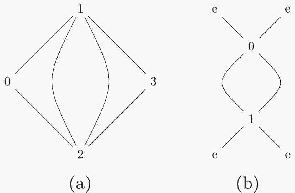First, one should consider a connected graph with $n$ vertices and label these $n$ vertices by the integers $0$ through $n-1$ at random. Therefore, the sequence can be constructed according to [35,36]:

For instance, Fig. 1(a) can be represented by $12|223|3|$. Otherwise, we can use the label "$e$" to describe the external lines in the diagrams. Moreover, the Nickel notation of Fig. 1(b) is $ee11|ee|$. With different labeling strategies, one diagram can be represented as different Nickel notations, which describe the same diagram up to a topological homeomorphism. For simplicity, the Nickel index algorithm can be used to find the "minimal" Nickel notation, which is called the Nickel index. Consequently, the diagram and its Nickel index are in a one-to-one correspondence. For instance, the Nickel index of Fig. 1(a) is $1123|23|||$. The package GraphState [35] is a useful tool for constructing the Nickel index. The details of the Nickel index algorithm can be found in Ref. [35].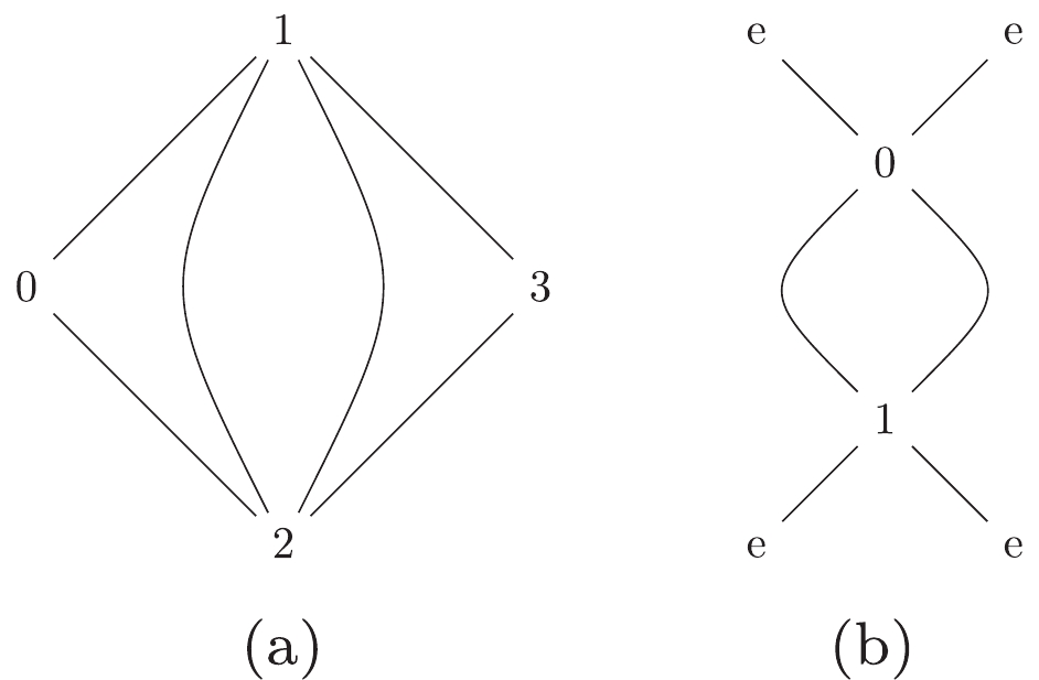

Figure 1

Figure 1.  Nickel notation and Nickel index.

DownLoad: Full-Size Img PowerPoint

In this paper, the topological structures of the diagrams with one vertex connecting to one or two external legs are regarded as equivalent. For instance, the topological structures of two diagrams in Fig. 2 can be regarded as equivalent.

Figure 2

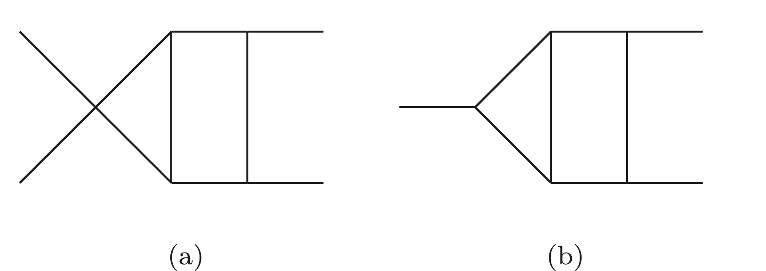
Figure 2.  Example of equivalent topological structures.

DownLoad: Full-Size Img PowerPoint

A Category ${\cal C}_1$

• I. INTRODUCTION
• II. CATEGORIZATION
•      A Category ${\cal C}_1$
•      B Category ${\cal C}_2$
•      C Category ${\cal C}_3$
•      D Category ${\cal C}_4$
•      E Category ${\cal C}_5$
•      F Category ${\cal C}_6$
• III. CONCLUSION
• ACKNOWLEDGMENTS

The category ${\cal C}_1$ includes 7908 Feynman diagrams that can be factorized into two one-loop diagrams. Therefore, the calculations of diagrams in ${\cal C}_1$ can be regarded as one-loop level calculations. According to the topologies of loop structures in ${\cal C}_1$, they are categorized into 3 subcategories.

The subcategory ${\cal C}_{1,1}$ includes 2117 diagrams which contain at least one one-loop vacuum bubble diagram. Furthermore, ${\cal C}_{1,1,a}$ includes 2055 diagrams, and ${\cal C}_{1,1,b}$ includes 62 diagrams. In ${\cal C}_{1,1,b}$, there are 14 diagrams whose amplitudes are equal to zero. ${\cal C}_{1,1,a}^{ind}$ has 449 independent diagrams, and ${\cal C}_{1,1,b}^{ind}$ has 36 independent diagrams. We choose diagram #47 as the representative of ${\cal C}_{1,1,a}$ and diagram #4418 as the representative of ${\cal C}_{1,1,b}$.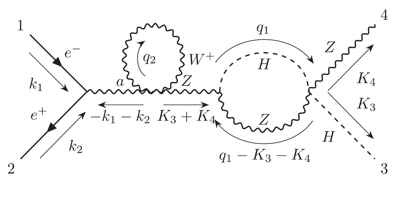

Figure 3

Figure 3.  Diagram #47 (representative of $\mathcal C_{1,1,a}$).

DownLoad: Full-Size Img PowerPoint

Figure 4

Figure 4.  Diagram #4418 (representative of $\mathcal C_{1,1,b}$).

DownLoad: Full-Size Img PowerPoint

The subcategory ${\cal C}_{1,2}$ includes 5513 diagrams that contain self-energy corrections. The diagrams ${\cal C}_{1,2}$ do not contain vacuum bubble diagrams. ${\cal C}_{1,2,a}$ includes 4775 diagrams, and ${\cal C}_{1,2,b}$ includes 738 diagrams. In ${\cal C}_{1,2,b}$, there are 131 diagrams whose amplitudes are equal to zero. ${\cal C}_{1,2,a}^{ind}$ has 740 independent diagrams, and ${\cal C}_{1,2,b}^{ind}$ has 278 independent diagrams. We choose diagram #36 as the representative of ${\cal C}_{1,2,a}$ and diagram #1035 as the representative of ${\cal C}_{1,2,b}$.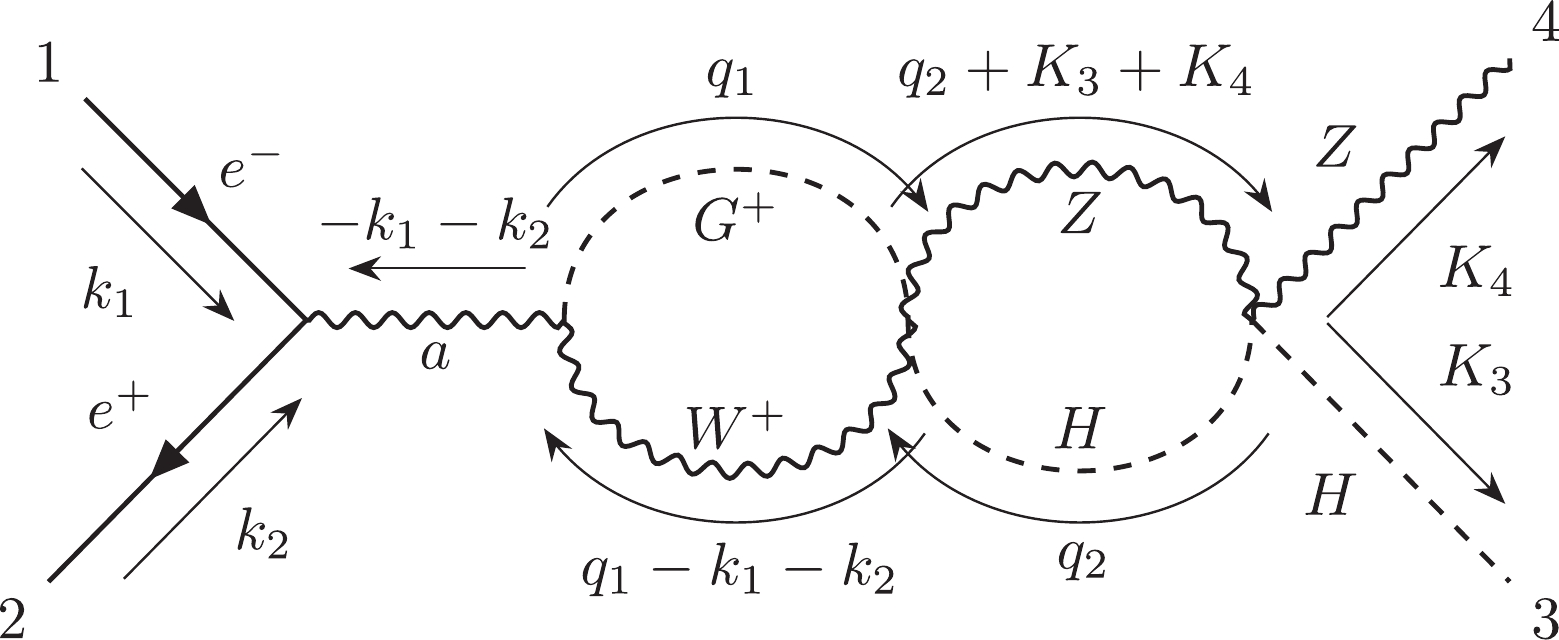

Figure 5

Figure 5.  Diagram #36 (representative of ${\cal C}_{1,2,a}$).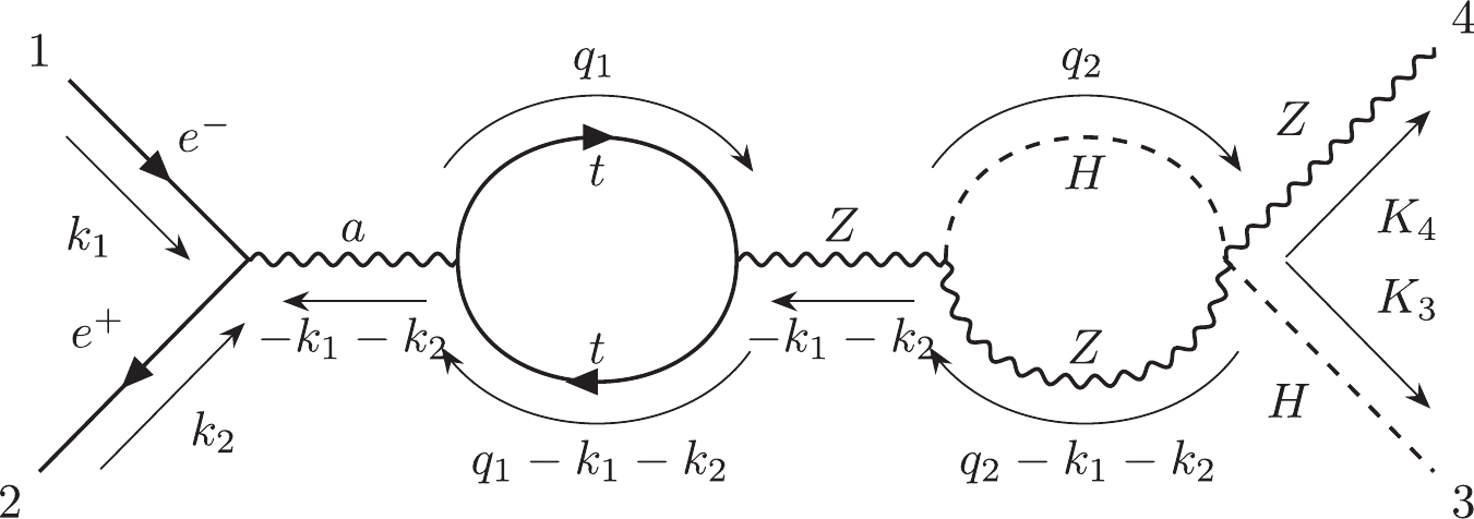

DownLoad: Full-Size Img PowerPoint

Figure 6

Figure 6.  Diagram #1035 (representative of ${\cal C}_{1,2,b}$).

DownLoad: Full-Size Img PowerPoint

The subcategory ${\cal C}_{1,3}$ includes 278 diagrams, which contain two vertex corrections. ${\cal C}_{1,3,a}$ includes 260 diagrams, and ${\cal C}_{1,3,b}$ includes 18 diagrams. ${\cal C}_{1,3,a}^{ind}$ has 68 independent diagrams, and ${\cal C}_{1,3,b}^{ind}$ has 14 independent diagrams. We choose diagram #6983 as the representative of ${\cal C}_{1,3,a}$ and diagram #23660 as the representative of ${\cal C}_{1,3,b}$.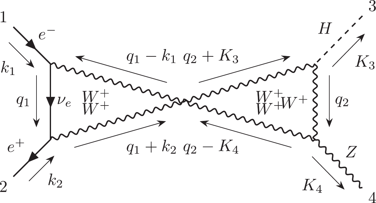

Figure 7

Figure 7.  Diagram #6983 (representative of ${\cal C}_{1,3,a}$).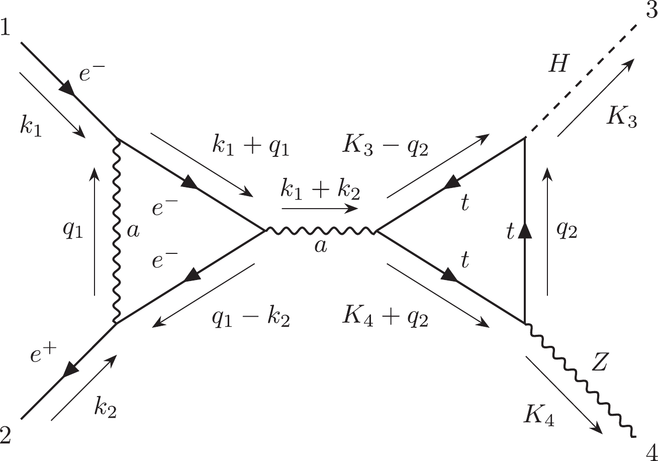

DownLoad: Full-Size Img PowerPoint

Figure 8

Figure 8.  Diagram #23660 (representative of ${\cal C}_{1,3,b}$).

DownLoad: Full-Size Img PowerPoint

B Category ${\cal C}_2$

• I. INTRODUCTION
• II. CATEGORIZATION
•      A Category ${\cal C}_1$
•      B Category ${\cal C}_2$
•      C Category ${\cal C}_3$
•      D Category ${\cal C}_4$
•      E Category ${\cal C}_5$
•      F Category ${\cal C}_6$
• III. CONCLUSION
• ACKNOWLEDGMENTS

The category ${\cal C}_2$ includes non-factorizable two-loop Feynman diagrams with three denominators. We found that all diagrams in ${\cal C}_{2}$ are two-loop self-energy diagrams. ${\cal C}_2$ includes 18 diagrams, none of which contains a top quark. ${\cal C}_{2}^{ind}$ has 8 independent diagrams. We choose diagram #519 as the representative of ${\cal C}_2$.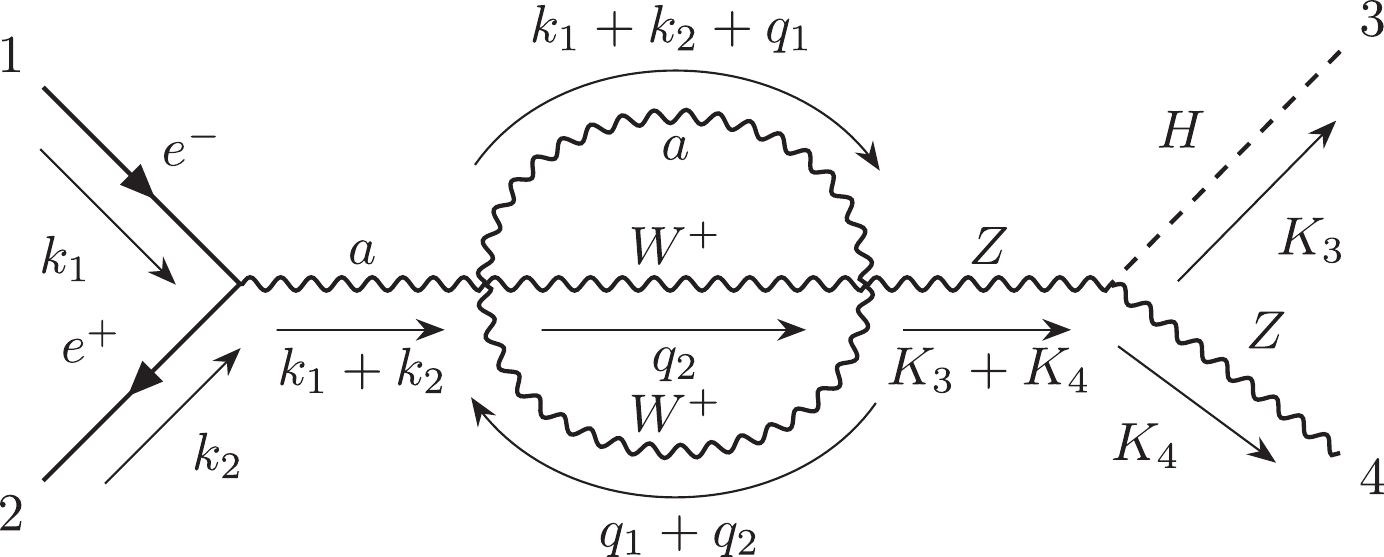

Figure 9

Figure 9.  Diagram #519 (representative of ${\cal C}_{2}$).

DownLoad: Full-Size Img PowerPoint

C Category ${\cal C}_3$

• I. INTRODUCTION
• II. CATEGORIZATION
•      A Category ${\cal C}_1$
•      B Category ${\cal C}_2$
•      C Category ${\cal C}_3$
•      D Category ${\cal C}_4$
•      E Category ${\cal C}_5$
•      F Category ${\cal C}_6$
• III. CONCLUSION
• ACKNOWLEDGMENTS

The category ${\cal C}_3$ includes 593 non-factorizable two-loop Feynman diagrams with four denominators. According to the topologies of loop structures in ${\cal C}_3$, we categorize them into 3 subcategories.

The subcategory ${\cal C}_{3,1}$ includes 142 diagrams that can be separated into the tree-level diagrams and the two-loop vacuum bubble diagrams. The topology of their loop structures can be noted as $112|2||$ in the Nickel index. The calculation of the two-loop vacuum bubble diagram has been well studied [38]. ${\cal C}_{3,1}^{ind}$ has 51 independent diagrams. We choose diagram #3961 as the representative of ${\cal C}_{3,1}$.

Figure 10

Figure 10.  Diagram #3961 (representative of ${\cal C}_{3,1}$).

DownLoad: Full-Size Img PowerPoint

The subcategory ${\cal C}_{3,2}$ includes 337 two-loop self-energy diagrams, none of which contains the top quark. ${\cal C}_{3,2}^{ind}$ has 93 independent diagrams. We choose diagram #1 as the representative of ${\cal C}_{3,2}$.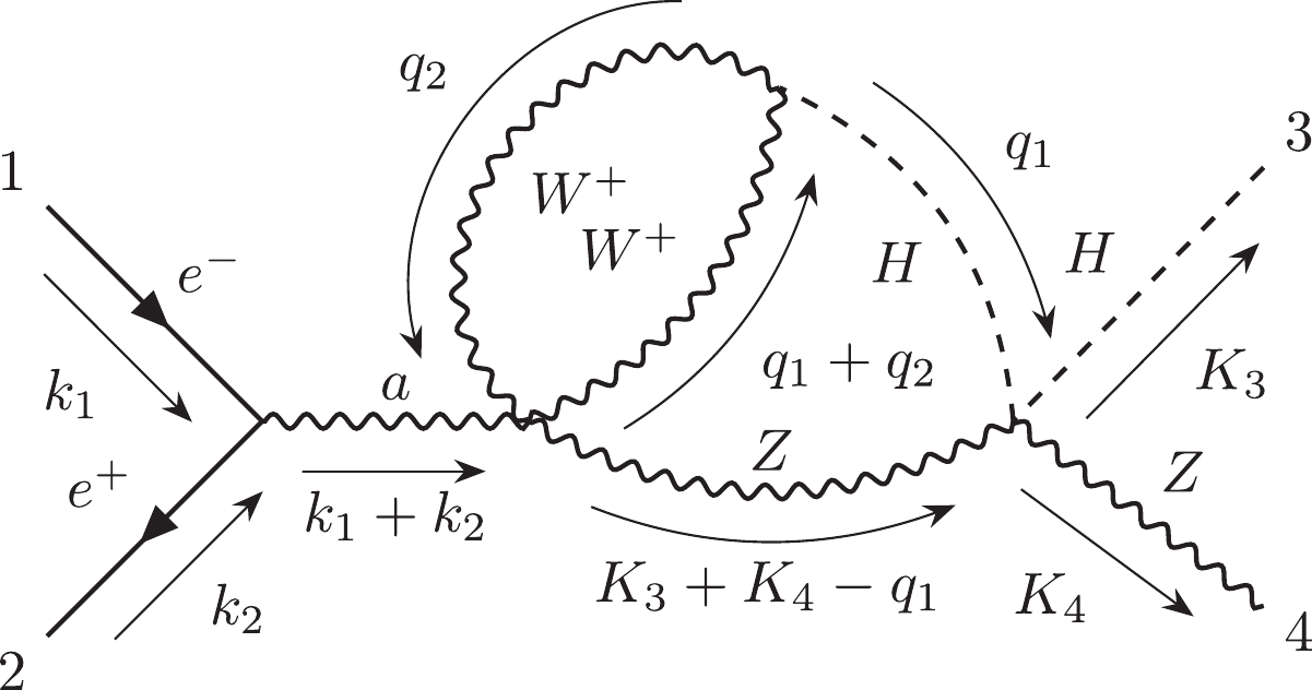

Figure 11

Figure 11.  Diagram #1 (representative of ${\cal C}_{3,2}$).

DownLoad: Full-Size Img PowerPoint

The subcategory ${\cal C}_{3,3}$ includes 114 two-loop vertex correction diagrams, none of which contains the top quark. The topology of their loop structures can be noted as $e112|e2|e|$ in the Nickel index. The denominators of diagrams in ${\cal C}_{3,3}$ only depend on two external momenta. ${\cal C}_{3,3}^{ind}$ has 24 independent diagrams. We choose diagram #191 as the representative of ${\cal C}_{3,3}$.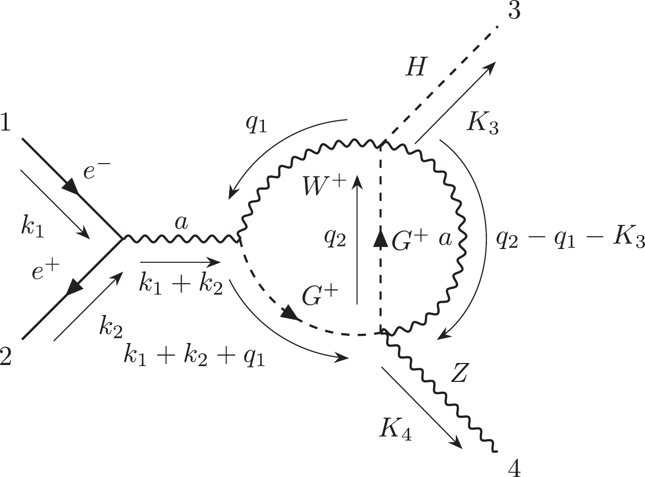

Figure 12

Figure 12.  Diagram #191 (representative of ${\cal C}_{3,3}$).

DownLoad: Full-Size Img PowerPoint

D Category ${\cal C}_4$

• I. INTRODUCTION
• II. CATEGORIZATION
•      A Category ${\cal C}_1$
•      B Category ${\cal C}_2$
•      C Category ${\cal C}_3$
•      D Category ${\cal C}_4$
•      E Category ${\cal C}_5$
•      F Category ${\cal C}_6$
• III. CONCLUSION
• ACKNOWLEDGMENTS

The category ${\cal C}_4$ includes 4773 non-factorizable two-loop Feynman diagrams with five denominators. According to the topologies of loop structures in ${\cal C}_4$, we categorize them into 3 subcategories.

The subcategory ${\cal C}_{4,1}$ includes 3266 two-loop self-energy diagrams, some of which contain the top quark. ${\cal C}_{4,1,a}$ includes 2565 diagrams and ${\cal C}_{4,1,b}$ includes 701 diagrams. ${\cal C}_{4,1,a}^{ind}$ has 753 independent diagrams, and ${\cal C}_{4,1,b}^{ind}$ has 249 independent diagrams. We choose diagram #603 as the representative of ${\cal C}_{4,1,a}$ and diagram #611 as the representative of ${\cal C}_{4,1,b}$.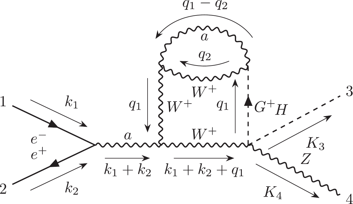

Figure 13

Figure 13.  Diagram #603 (representative of ${\cal C}_{4,1,a}$).

DownLoad: Full-Size Img PowerPoint

Figure 14

Figure 14.  Diagram #611 (representative of ${\cal C}_{4,1,b}$).

DownLoad: Full-Size Img PowerPoint

The subcategory ${\cal C}_{4,2}$ includes 637 two-loop vertex correction diagrams, none of which contains the top quark. The topology of their loop structures can be noted as $e12|e23|3|e|$ in the Nickel index. The denominators of diagrams in ${\cal C}_{4,2}$ only depend on two external momenta. ${\cal C}_{4,2}^{ind}$ has 140 independent diagrams. We choose diagram #2676 as the representative of ${\cal C}_{4,2}$.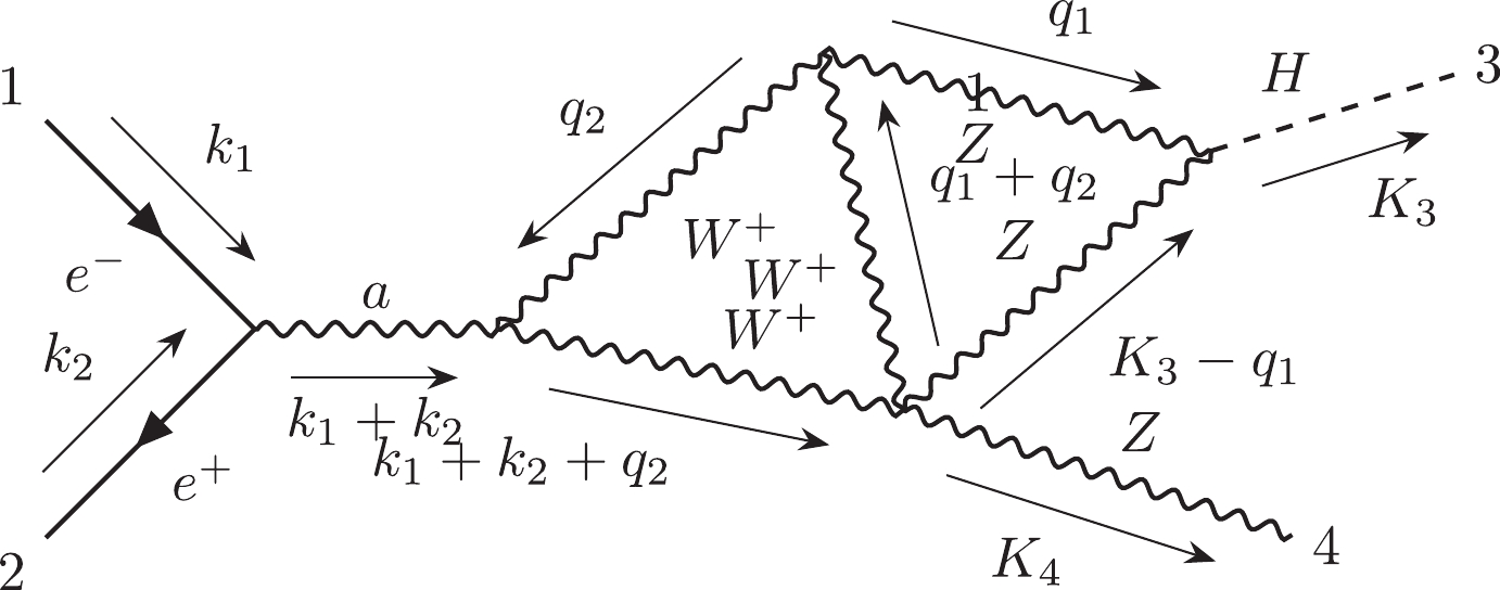

Figure 15

Figure 15.  Diagram #2676 (representative of ${\cal C}_{4,2}$).

DownLoad: Full-Size Img PowerPoint

The subcategory ${\cal C}_{4,3}$ includes 870 two-loop vertex correction diagrams, none of which contains the top quark. The topology of their loop structures can be noted as $e112|3|e3|e|$ in the Nickel index. The denominators of diagrams in ${\cal C}_{4,3}$ only depend on two external momenta. ${\cal C}_{4,3}^{ind}$ has 278 independent diagrams. We choose diagram #3063 as the representative of ${\cal C}_{4,3}$.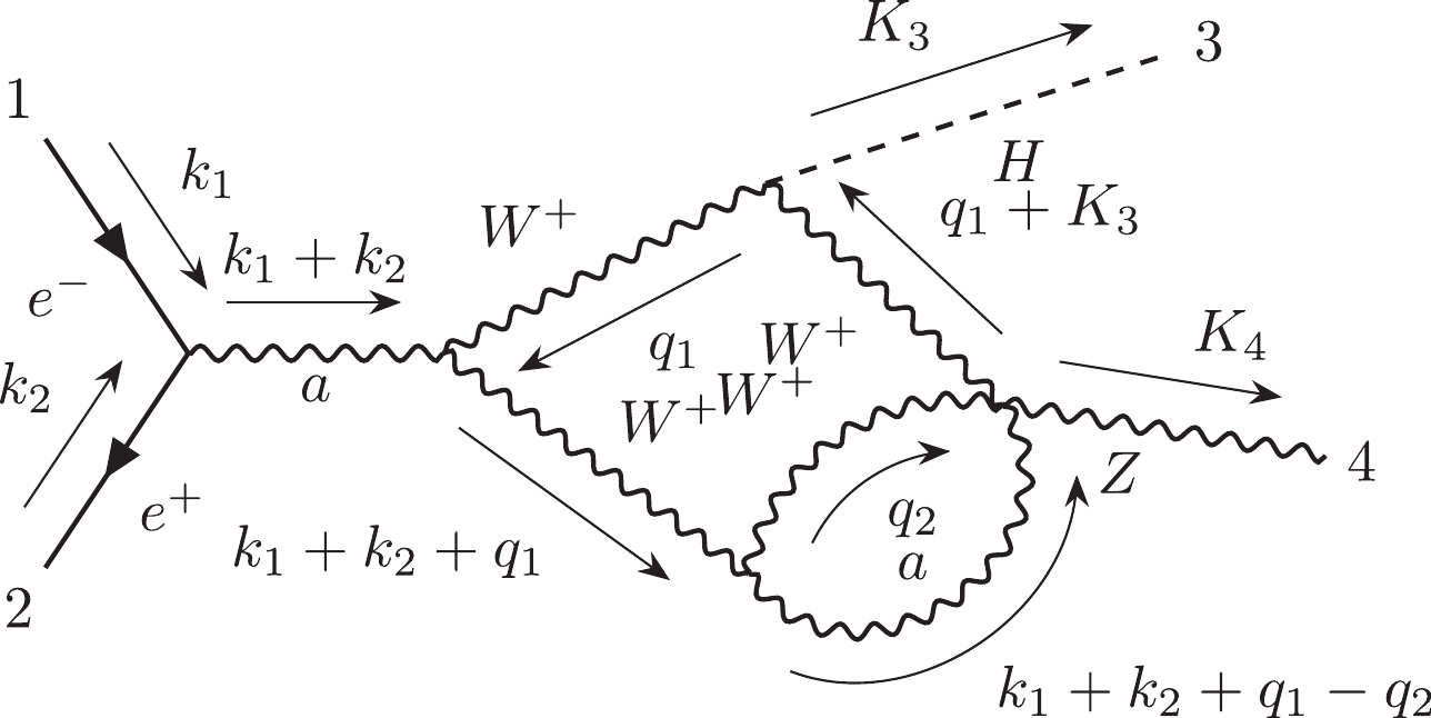

Figure 16

Figure 16.  Diagram #3063 (representative of ${\cal C}_{4,3}$).

DownLoad: Full-Size Img PowerPoint

E Category ${\cal C}_5$

• I. INTRODUCTION
• II. CATEGORIZATION
•      A Category ${\cal C}_1$
•      B Category ${\cal C}_2$
•      C Category ${\cal C}_3$
•      D Category ${\cal C}_4$
•      E Category ${\cal C}_5$
•      F Category ${\cal C}_6$
• III. CONCLUSION
• ACKNOWLEDGMENTS

The category ${\cal C}_5$ includes 9835 non-factorizable two-loop Feynman diagrams with six denominators. According to the topologies of loop structures in ${\cal C}_5$, we categorize them into six subcategories.

The subcategory ${\cal C}_{5,1}$ includes two-loop planar triangle diagrams. The topology of their loop structures can be noted as $e12|e3|34|4|e|$ in the Nickel index. The denominators of diagrams in ${\cal C}_{5,1}$ only depend on two external momenta. ${\cal C}_{5,1}$ includes 4897 diagrams, some of which contain the top quark. Then, ${\cal C}_{5,1,a}$ includes 3966 diagrams, and ${\cal C}_{5,1,b}$ includes 931 diagrams. ${\cal C}_{5,1,a}^{ind}$ has 1039 independent diagrams, and ${\cal C}_{5,1,b}^{ind}$ has 397 independent diagrams. We choose diagram #1325 as the representative of ${\cal C}_{5,1,a}$ and diagram #16206 as the representative of ${\cal C}_{5,1,b}$.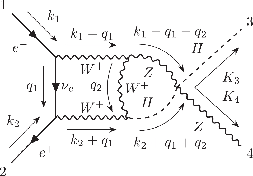

Figure 17

Figure 17.  Diagram #1325 (representative of ${\cal C}_{5,1,a}$).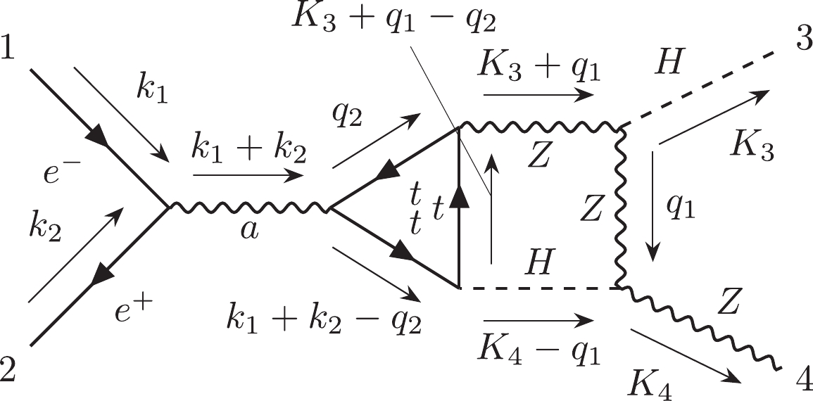

DownLoad: Full-Size Img PowerPoint

Figure 18

Figure 18.  Diagram #16206 (representative of ${\cal C}_{5,1,b}$).

DownLoad: Full-Size Img PowerPoint

The subcategory ${\cal C}_{5,2}$ includes 184 two-loop planar diagrams, none of which contains the top quark. The topology of their loop structures can be noted as $e12|e23|4|e4|e|$ in the Nickel index. ${\cal C}_{5,2}^{ind}$ has 90 independent diagrams. We choose diagram #3613 as the representative of ${\cal C}_{5,2}$.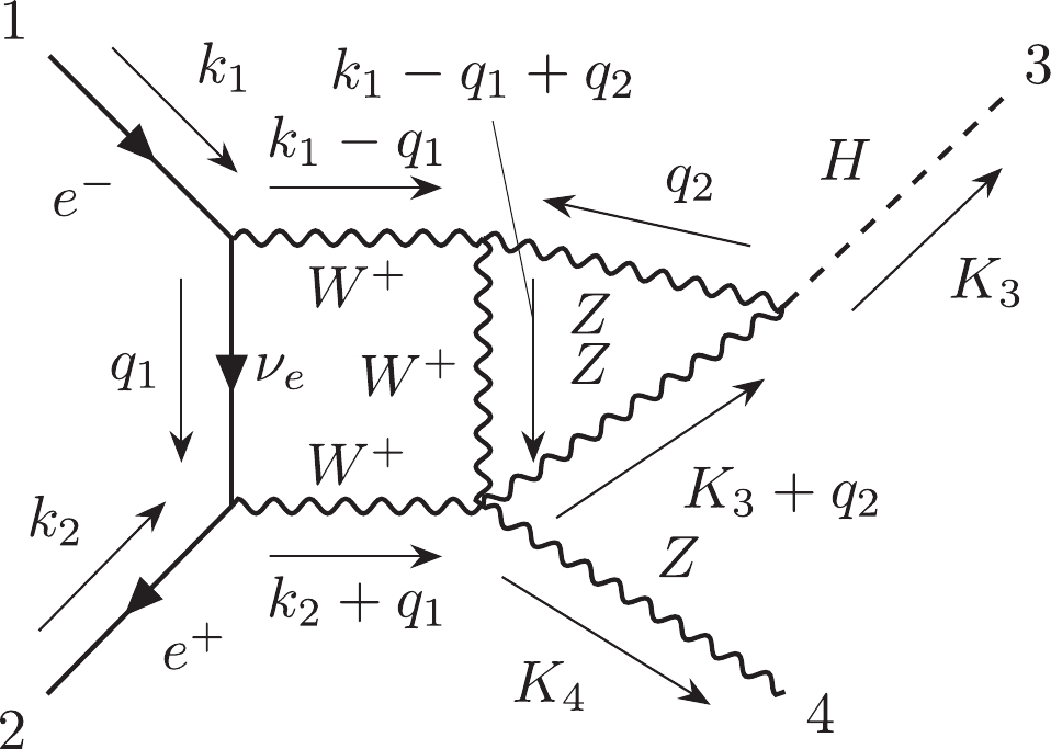

Figure 19

Figure 19.  Diagram #3613 (representative of ${\cal C}_{5,2}$).

DownLoad: Full-Size Img PowerPoint

The subcategory ${\cal C}_{5,3}$ includes two-loop planar diagrams. The topology of their loop structures can be noted as $e12|e3|e4|44||$ in the Nickel index. The denominators of diagrams in ${\cal C}_{5,3}$ only depend on two external momenta. ${\cal C}_{5,3}$ includes 4067 diagrams, some of which contains the top quark. ${\cal C}_{5,3,a}$ includes 3260 diagrams, and ${\cal C}_{5,3,b}$ includes 807 diagrams. In ${\cal C}_{5,3,b}$, there are 131 diagrams whose amplitudes are equal to zero. ${\cal C}_{5,3,a}^{ind}$ has 1077 independent diagrams, and ${\cal C}_{5,3,b}^{ind}$ has 264 independent diagrams. We choose diagram #14794 as the representative of ${\cal C}_{5,3,a}$ and diagram #14812 as the representative of ${\cal C}_{5,3,b}$.

Figure 20

Figure 20.  Diagram #14794 (representative of ${\cal C}_{5,3,a}$).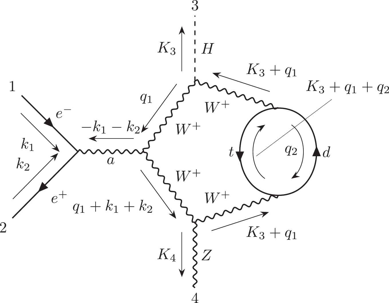

DownLoad: Full-Size Img PowerPoint

Figure 21

Figure 21.  Diagram #14812 (representative of ${\cal C}_{5,3,b}$).

DownLoad: Full-Size Img PowerPoint

The subcategory ${\cal C}_{5,4}$ includes two-loop planar diagrams. The topology of their loop structures can be noted as $e112|3|e4|e4|e|$ in the Nickel index. ${\cal C}_{5,4}$ includes 116 Feynman diagrams, none of which contains the top quark. ${\cal C}_{5,4}^{ind}$ has 70 independent diagrams. We choose diagram #3845 as a representative of ${\cal C}_{5,4}$.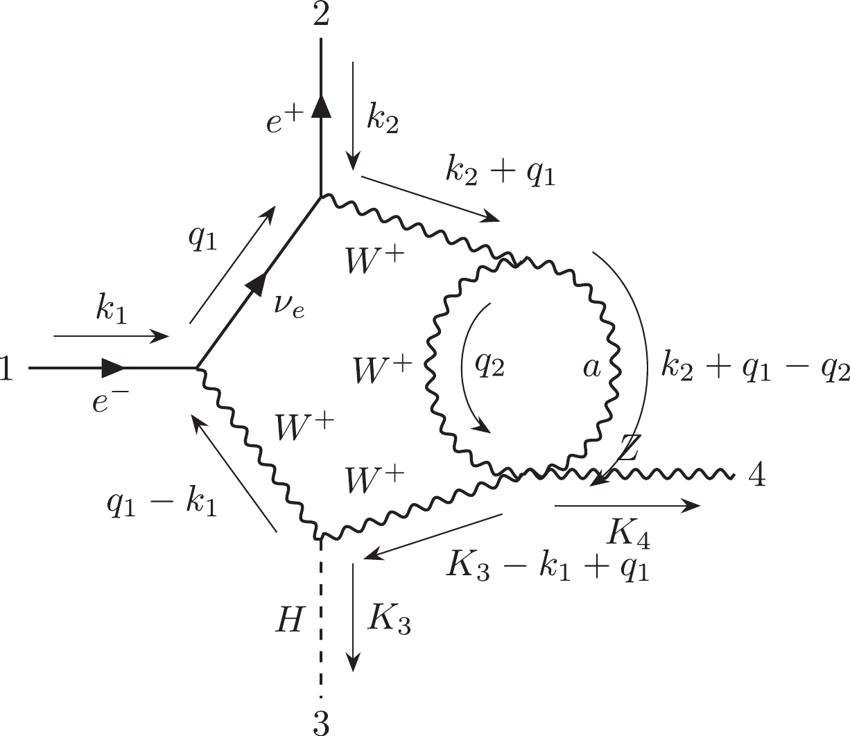

Figure 22

Figure 22.  Diagram #3845 (representative of ${\cal C}_{5,4}$).

DownLoad: Full-Size Img PowerPoint

The subcategory ${\cal C}_{5,5}$ includes two-loop non-planar triangle diagrams. The topology of their loop structures can be noted as $e12|34|34|e|e|$ in the Nickel index. The denominators of diagrams in ${\cal C}_{5,5}$ only depend on two external momenta. ${\cal C}_{5,5}$ includes 560 diagrams, some of which contain the top quark. ${\cal C}_{5,5,a}$ includes 442 diagrams and ${\cal C}_{5,5,b}$ includes 118 diagrams. ${\cal C}_{5,5,a}^{ind}$ has 140 independent diagrams and ${\cal C}_{5,5,b}^{ind}$ has 54 independent diagrams. We choose diagram #1267 as the representative of ${\cal C}_{5,5,a}$ and diagram #11100 as the representative of ${\cal C}_{5,5,b}$.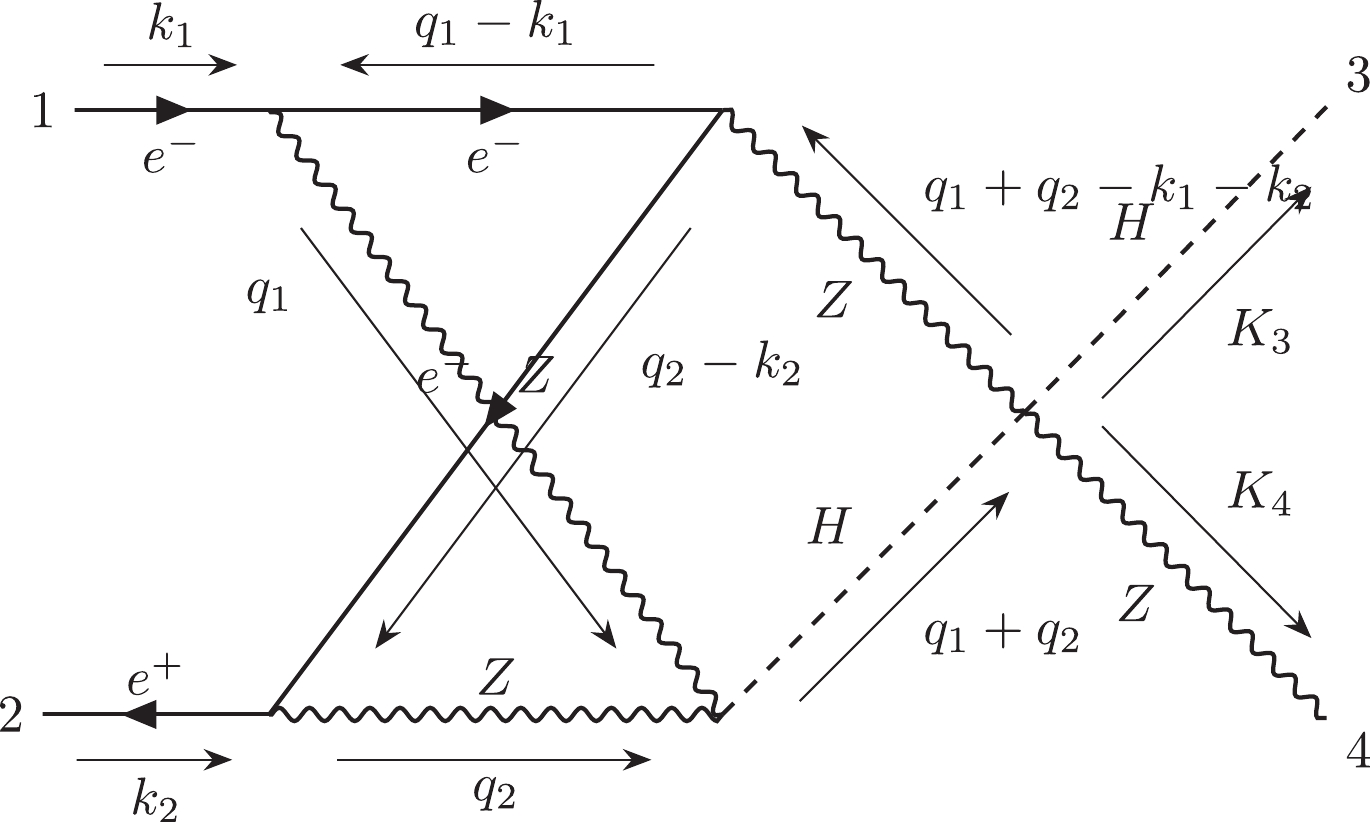

Figure 23

Figure 23.  Diagram #1267 (representative of ${\cal C}_{5,5,a}$).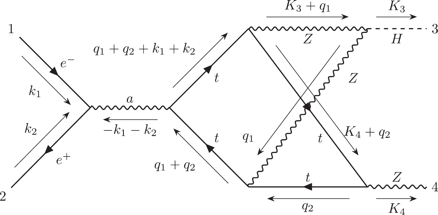

DownLoad: Full-Size Img PowerPoint

Figure 24

Figure 24.  Diagram #11100 (representative of ${\cal C}_{5,5,b}$).

DownLoad: Full-Size Img PowerPoint

The subcategory ${\cal C}_{5,6}$ includes two-loop non-planar diagrams. The topology of their loop structures can be noted as $e12|e34|34|e|e|$ in the Nickel index. ${\cal C}_{5,6}$ includes 11 diagrams, none of which contains the top quark. ${\cal C}_{5,6}^{ind}$ has 8 independent diagrams. We choose diagram #3602 as the representative of ${\cal C}_{5,6}$.

Figure 25

Figure 25.  Diagram #3602 (representative of ${\cal C}_{5,6}$).

DownLoad: Full-Size Img PowerPoint

F Category ${\cal C}_6$

• I. INTRODUCTION
• II. CATEGORIZATION
•      A Category ${\cal C}_1$
•      B Category ${\cal C}_2$
•      C Category ${\cal C}_3$
•      D Category ${\cal C}_4$
•      E Category ${\cal C}_5$
•      F Category ${\cal C}_6$
• III. CONCLUSION
• ACKNOWLEDGMENTS

The category ${\cal C}_6$ includes 2250 non-factorizable two-loop Feynman diagrams with seven denominators. According to the topologies of loop structures in ${\cal C}_6$, we categorize them into 4 subcategories.

The subcategory ${\cal C}_{6,1}$ includes 446 two-loop planar double-box diagrams. The topology of their loop structures can be noted as $e12|e3|34|5|e5|e|$ in the Nickel index. ${\cal C}_{6,1,a}$ includes 424 diagrams, and ${\cal C}_{6,1,b}$ includes 22 diagrams. ${\cal C}_{6,1,a}^{ind}$ has 194 independent diagrams, and ${\cal C}_{6,1,b}^{ind}$ has 18 independent diagrams. We choose diagram #23202 as the representative of ${\cal C}_{6,1,a}$ and diagram #23228 as the representative of ${\cal C}_{6,1,b}$.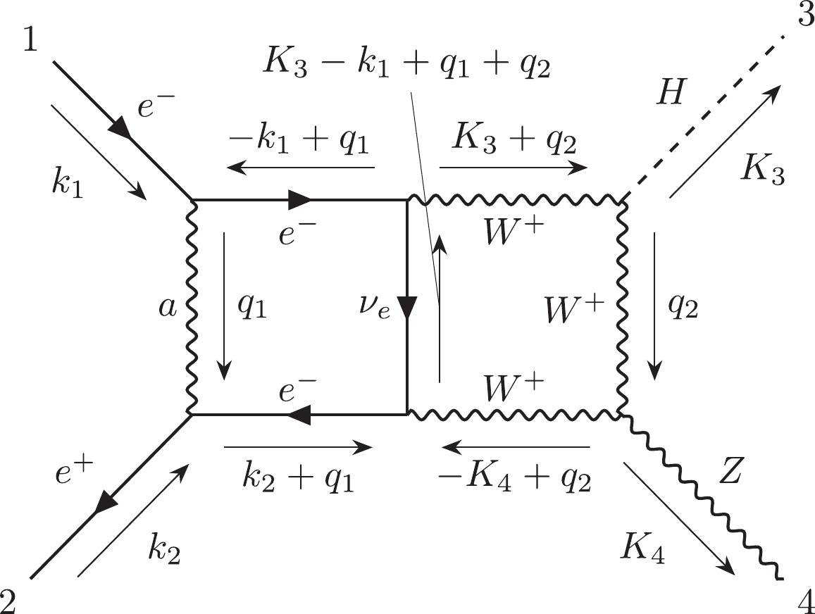

Figure 26

Figure 26.  Diagram #23202 (representative of ${\cal C}_{6,1,a}$).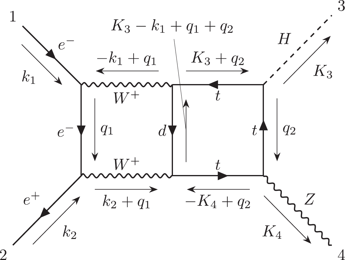

DownLoad: Full-Size Img PowerPoint

Figure 27

Figure 27.  Diagram #23228 (representative of ${\cal C}_{6,1,b}$).

DownLoad: Full-Size Img PowerPoint

The subcategory ${\cal C}_{6,2}$ includes 688 two-loop planar diagrams. The topology of their loop structures can be noted as $e1|22|3|e4|e5|e6||$ in the Nickel index. ${\cal C}_{6,2,a}$ includes 580 diagrams and ${\cal C}_{6,2,b}$ includes 108 diagrams. In ${\cal C}_{6,2,b}$, there are 4 diagrams whose amplitudes are equal to zero. ${\cal C}_{6,2,a}^{ind}$ has 299 independent diagrams, and ${\cal C}_{6,2,b}^{ind}$ has 48 independent diagrams. We choose diagram #24690 as the representative of ${\cal C}_{6,2,a}$ and diagram #24708 as the representative of ${\cal C}_{6,2,b}$.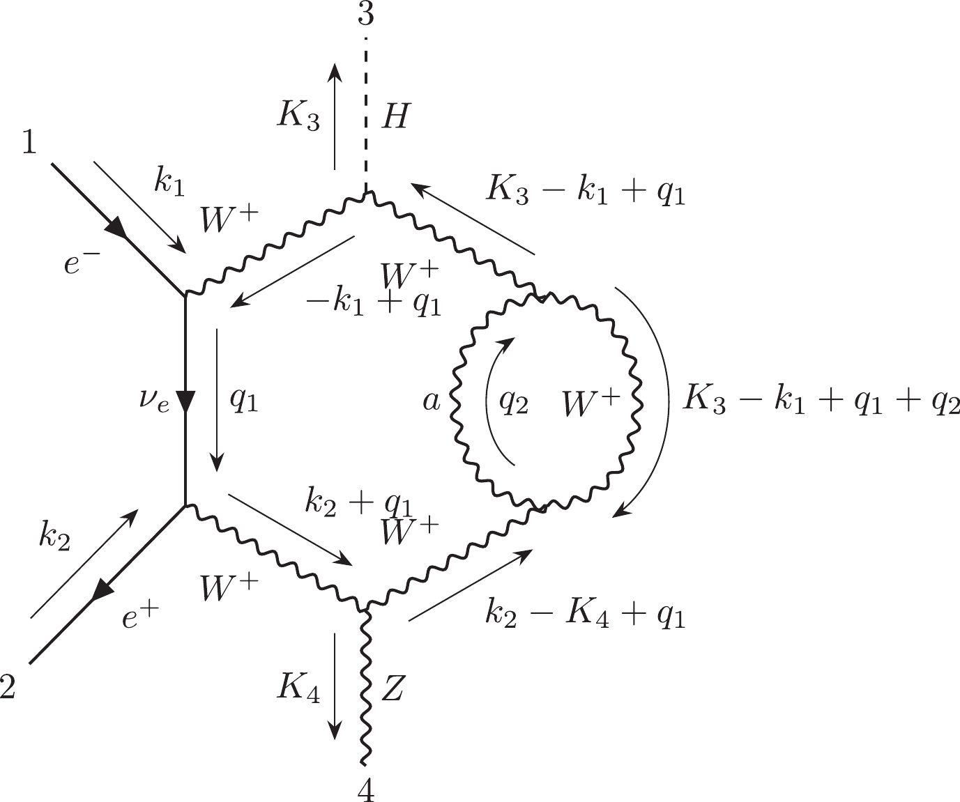

Figure 28

Figure 28.  Diagram #24690 (representative of ${\cal C}_{6,2,a}$).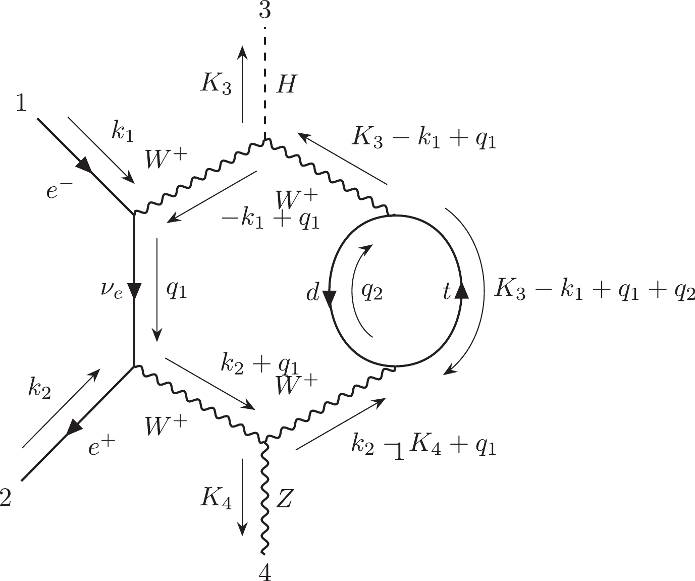

DownLoad: Full-Size Img PowerPoint

Figure 29

Figure 29.  Diagram #24708 (representative of ${\cal C}_{6,2,b}$).

DownLoad: Full-Size Img PowerPoint

The subcategory ${\cal C}_{6,3}$ includes 804 two-loop planar diagrams. The topology of their loop structures can be represented as $e12|e3|e4|45|5|e|$ in the Nickel index. ${\cal C}_{6,3,a}$ includes 733 diagrams, and ${\cal C}_{6,2,b}$ includes 71 diagrams. ${\cal C}_{6,3,a}^{ind}$ has 302 independent diagrams, and ${\cal C}_{6,3,b}^{ind}$ has 42 independent diagrams. We choose diagram #23886 as the representative of ${\cal C}_{6,3,a}$ and diagram #23907 as the representative of ${\cal C}_{6,3,b}$.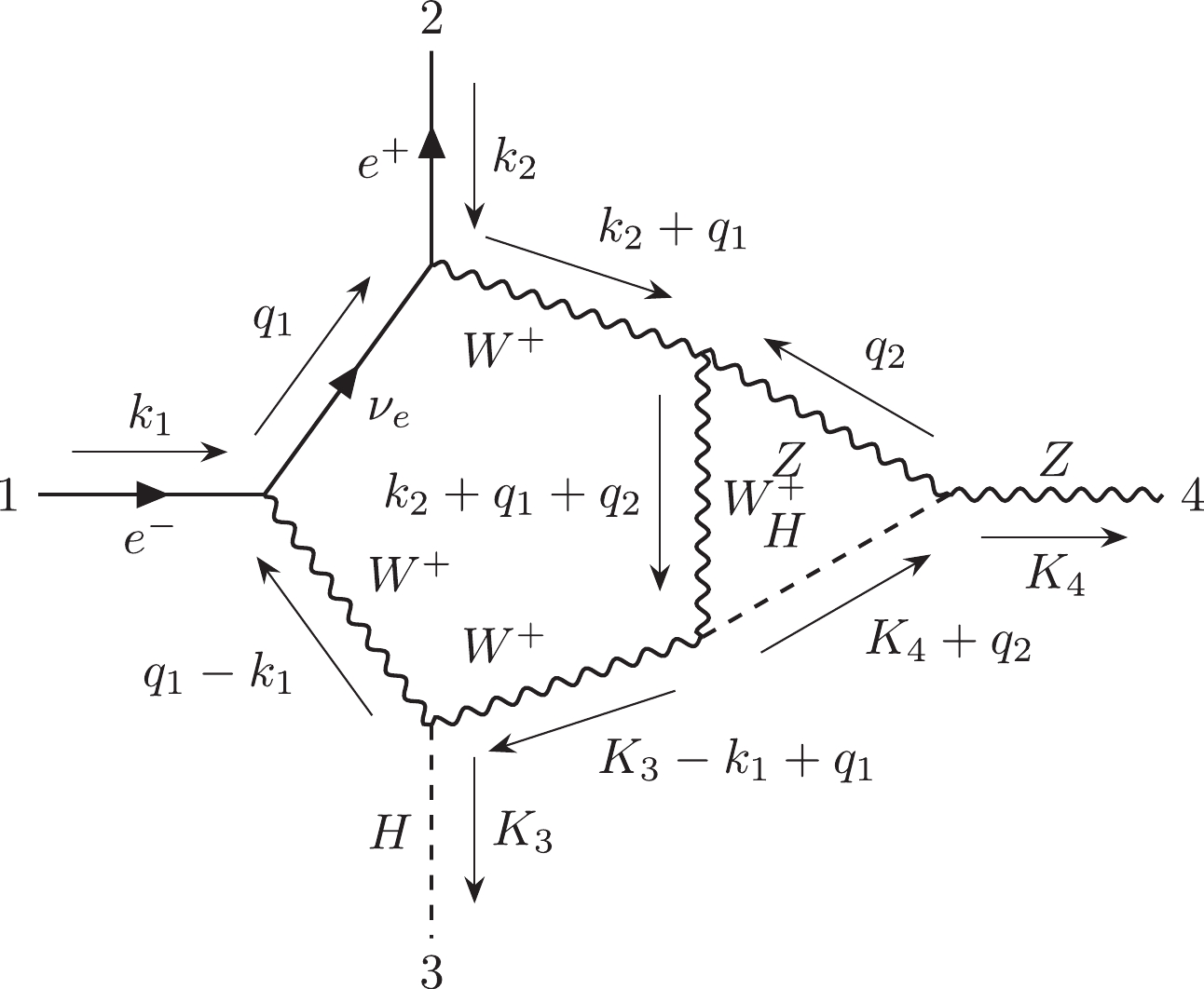

Figure 30

Figure 30.  Diagram #23886 (representative of ${\cal C}_{6,3,a}$).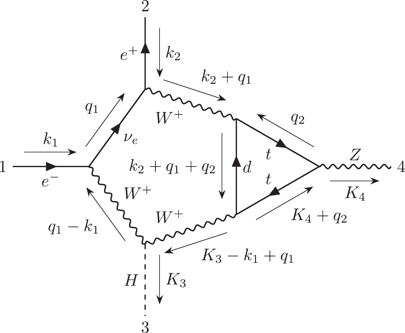

DownLoad: Full-Size Img PowerPoint

Figure 31

Figure 31.  Diagram #23907 (representative of ${\cal C}_{6,3,b}$).

DownLoad: Full-Size Img PowerPoint

The subcategory${\cal C}_{6,4}$ is the most challenging subcategory which includes 312 two-loop non-planar double-box diagrams. The topology of their loop structures can be noted as $e12|e3|45|45|e|e|$ in the Nickel index. ${\cal C}_{6,4,a}$ includes 301 diagrams, and ${\cal C}_{6,4,b}$ includes 11 diagrams. ${\cal C}_{6,4,a}^{ind}$ has 146 independent diagrams, and ${\cal C}_{6,4,b}^{ind}$ has 9 independent diagrams. We choose diagram #22890 as the representative of ${\cal C}_{6,4,a}$ and diagram #22909 as the representative of ${\cal C}_{6,4,b}$.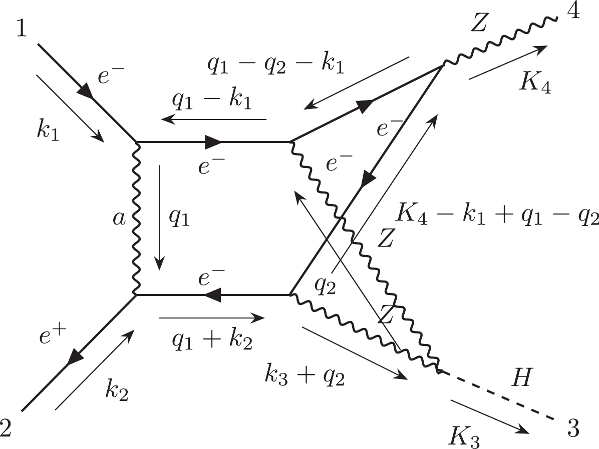

Figure 32

Figure 32.  Diagram #22890 (representative of ${\cal C}_{6,4,a}$).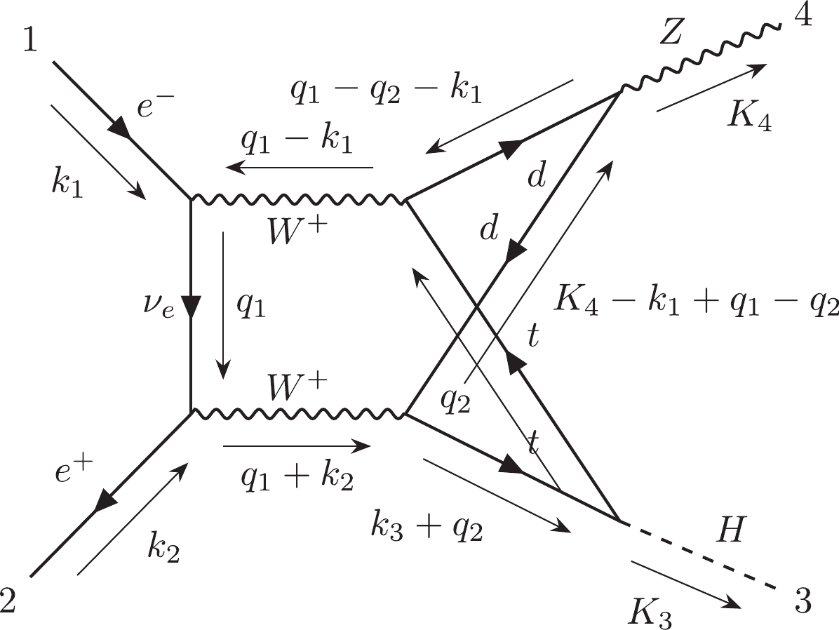

DownLoad: Full-Size Img PowerPoint

Figure 33

Figure 33.  Diagram #22909 (representative of ${\cal C}_{6,4,b}$).

DownLoad: Full-Size Img PowerPoint

Finally, the information for all subcategories has been summarized in Table 1.

Table 1

Table 1.  Summary table for all subcategories.

subcategory name	number of diagrams	number of denominators	non-planar diagrams	contains the top quark	number of independent diagrams
$C_{1,1}$	2117	−	No	Yes	485
$C_{1,2}$	5513	−	No	Yes	1018
$C_{1,3}$	278	−	No	Yes	82
$C_{2}$	18	3	No	No	8
$C_{3,1}$	142	4	No	No	51
$C_{3,2}$	337	4	No	No	93
$C_{3,3}$	114	4	No	No	24
$C_{4,1}$	3266	5	No	Yes	1002
$C_{4,2}$	637	5	No	No	140
$C_{4,3}$	870	5	No	No	278
$C_{5,1}$	4897	6	No	Yes	1436
$C_{5,2}$	184	6	No	No	90
$C_{5,3}$	4067	6	No	Yes	1341
$C_{5,4}$	116	6	No	No	70
$C_{5,5}$	560	6	Yes	Yes	194
$C_{5,6}$	11	6	Yes	No	8
$C_{6,1}$	446	7	No	Yes	212
$C_{6,2}$	688	7	No	Yes	347
$C_{6,3}$	804	7	No	Yes	344
$C_{6,4}$	312	7	Yes	Yes	155

DownLoad: CSV

Show Table

III. CONCLUSION

• I. INTRODUCTION
• II. CATEGORIZATION
•      A Category ${\cal C}_1$
•      B Category ${\cal C}_2$
•      C Category ${\cal C}_3$
•      D Category ${\cal C}_4$
•      E Category ${\cal C}_5$
•      F Category ${\cal C}_6$
• III. CONCLUSION
• ACKNOWLEDGMENTS

In this paper, we categorize the two-loop Feynman diagrams contributing to the ${\cal O}(\alpha^2)$ corrections in the Higgsstrahlung $e^+e^- \rightarrow ZH$ into 6 categories and numerous subcategories. The most challenging subcategory is ${\cal C}_{6,4}$, which includes 312 two-loop non-planar double-box diagrams. There are only 155 independent diagrams in ${\cal C}_{6,4}$. We hope that the calculations of these Feynman diagrams can be conveniently organized with the help of this categorization.

ACKNOWLEDGMENTS

• I. INTRODUCTION
• II. CATEGORIZATION
•      A Category ${\cal C}_1$
•      B Category ${\cal C}_2$
•      C Category ${\cal C}_3$
•      D Category ${\cal C}_4$
•      E Category ${\cal C}_5$
•      F Category ${\cal C}_6$
• III. CONCLUSION
• ACKNOWLEDGMENTS

The authors would like to thank Ayres Freitas, Hao Liang, and Tao Liu for helpful discussions.

References