


 Abstract
 HTML
HTML Reference
 Related
 PDF
PDF


-
Solar neutrinos, produced during nuclear fusion in the solar core, have played an important role in the history of neutrino physics, from the first observation and appearance of the solar neutrino problem at the Homestake experiment [1], to the measurements at Kamiokande [2], GALLEX/GNO [3, 4], and SAGE [5], and then to the precise measurements at Super-Kamiokande [6], SNO [7, 8], and Borexino [9]. In earlier radiochemical experiments, only the charged-current (CC) interactions of
$ \nu_{e} $ with the nuclei target could be measured. Subsequently, solar neutrinos were detected via the neutrino electron elastic scattering (ES) process in water Cherenkov or liquid scintillator (LS) detectors, which are predominantly sensitive to$ \nu_{e} $ , with lower cross sections for$ \nu_{\mu} $ and$ \nu_{\tau} $ . Exceptionally, the heavy water target used by SNO allowed observations of all three processes, including$ \nu-e $ ES, CC, and neutral-current (NC) interactions on deuterium [10]. The NC channel is equally sensitive to all active neutrino flavors, allowing a direct measurement of the$ ^8 $ B solar neutrino flux at production. Thus, SNO gave the first model-independent evidence of the solar neutrino flavor conversion and solved the solar neutrino problem.At present, there are still several open issues to be addressed in solar neutrino physics. The solar metallicity problem [11, 12] will profit from either precise measurements of the
$ ^7 $ Be and$ ^8 $ B solar neutrino fluxes, or the observation of solar neutrinos from the CNO cycle. On the elementary particle side, validation tests of the large mixing angle (LMA) Mikheyev-Smirnov-Wolfenstein (MSW) [13, 14] solution and the search for new physics beyond the standard scenario [15-18] constitute the main goals. The standard scenario of three neutrino mixing predicts a smooth upturn in the$ \nu_{e} $ survival probability ($ P_{ee} $ ) in the neutrino energy region between the high (MSW dominated) and low (vacuum dominated) ranges, and a sizable Day-Night asymmetry at the percentage level. However, by comparing the global analysis of solar neutrino data with the KamLAND reactor antineutrino data, we observe a mild inconsistency at the 2$ \sigma $ level for the mass-squared splitting$ \Delta m^2_{21} $ . The combined Super-K and SNO fitting favors$\Delta m^{2}_{21} = 4.8^{+1.3}_{-0.6}\times $ $ 10^{-5} $ eV$ ^{2} $ [19], while KamLAND gives$ \Delta m^{2}_{21} = 7.53^{+0.18}_{-0.18}\times $ $10^{-5} $ eV$ ^{2} $ [20]. From the latest results at the Neutrino 2020 conference [21], the inconsistency is reduced to around 1.4$ \sigma $ due to the larger statistics and the update of analysis methods.Determining whether this inconsistency is a statistical fluctuation or a physical effect beyond the standard neutrino oscillation framework requires further measurements. The Jiangmen Underground Neutrino Observatory (JUNO), a 20 kt multi-purpose underground liquid scintillator (LS) detector, can measure
$ \Delta m^2_{21} $ to an unprecedented sub-percent level using reactor antineutrinos [22]. Measurements of$ ^8 $ B solar neutrinos will also benefit, primarily because of the large target mass, which affords excellent self-shielding and comparable statistics to Super-K. A preliminary discussion of the radioactivity requirements and the cosmogenic isotope background can be found in the JUNO Yellow Book [22]. In this paper, we present a more comprehensive study with the following updates. The cosmogenic isotopes are better suppressed, with improved veto strategies. The analysis threshold for the recoil electrons can be decreased to 2 MeV, assuming an achievable intrinsic radioactivity background level, which compares favorably with the current world-best 3 MeV threshold at Borexino [23]. The lower threshold leads to larger signal statistics and a more sensitive examination of the spectrum distortion of recoil electrons. New measurement of the non-zero signal rate variation versus the solar zenith angle (Day-Night asymmetry) is also expected. After combining with the$ ^8 $ B neutrino flux from the SNO NC measurement, the$ \Delta m^2_{21} $ precision is expected to be similar to the current global fitting results [24]. This paper has the following structure. Sec. II presents the expected$ ^8 $ B neutrino signals in the JUNO detector. Sec. III describes the background budget, including the internal and external natural radioactivity, and the cosmogenic isotopes. Sec. IV summarizes the results of sensitivity studies. -
In LS detectors, the primary detection channel for solar neutrinos is their elastic scattering with electrons. The signal spectrum is predicted with the following steps: generation of neutrino flux and energy spectrum, considering oscillation in the Sun and the Earth; determination of the recoil electron rate and kinematics; and implementation of the detector response. A two-dimensional spectrum of signal counts with respect to the visible energy and the solar zenith angle is produced and utilized in sensitivity studies.
-
In this study, we assume an arrival
$ ^8 $ B neutrino flux of (5.25$ \pm0.20)\times10^6 $ /cm$ ^2 $ /s provided by the NC channel measurement at SNO [25]. The relatively small contribution ($ 8.25\times10^3 $ /cm$ ^2 $ /s) from$ hep $ neutrinos, produced by the capture of protons on$ ^3 $ He, is also included in the calculation of ES signals. The$ ^8 $ B and$ hep $ neutrino spectra are taken from Refs. [26, 27], as shown in Fig. 1. The neutrino spectrum shape uncertainties (a shift of approximately$ \pm $ 100 keV) are primarily due to the uncertain energy levels of$ ^8 $ Be excited states. The shape uncertainties are propagated into the energy-correlated systematic uncertainty on the recoil electron spectrum. The radial profile of the neutrino production in the Sun for each component is taken from Ref. [28].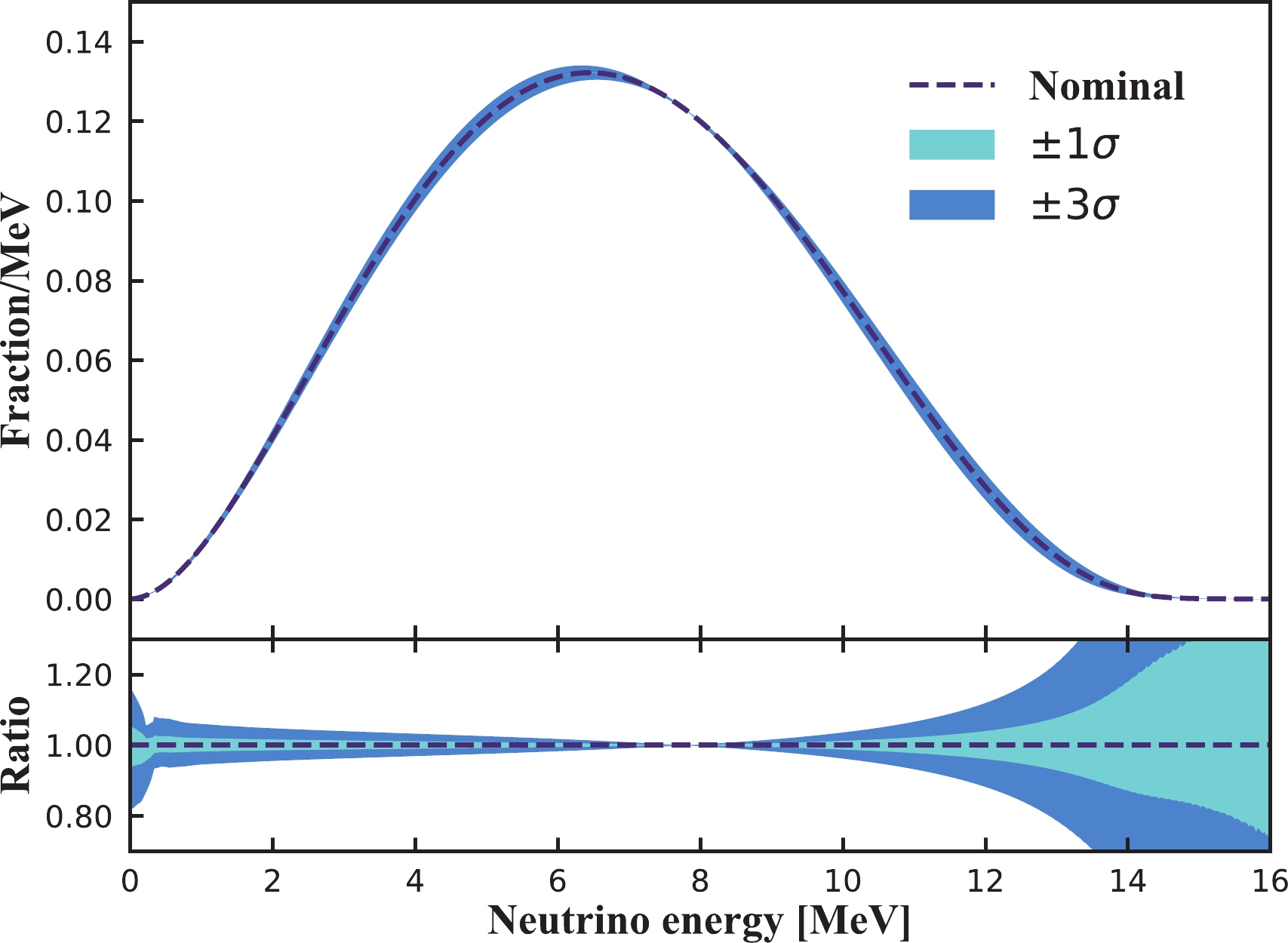
Figure 1. (color online)
$^8$ B$\nu_{e}$ spectrum together with the shape uncertainties. The data are taken from Ref. [26].Calculation of the solar neutrino oscillation in the Sun follows the standard MSW framework [13, 14]. The oscillation is affected by the coherent interactions with the medium via forward elastic weak CC scattering in the Sun. The neutrino evolution function can be modified by the electron density in the core, which is the so-called MSW effect. However, because of the slow change in electron density, the neutrino evolution function reduces to an adiabatic oscillation from the position where the neutrino is produced to the surface of the Sun. Moreover, the effects of evolution phases with respect to the effective mass eigenstates average out to be zero because of the sufficiently long propagation distance of the solar neutrinos, resulting in decoherent mass eigenstates prior to arrival on Earth. The survival probability of solar neutrinos is derived by taking all these effects into account.
During the Night, solar neutrinos must pass through the Earth prior to reaching the detector, which via the MSW effect can make the effective mass eigenstates coherent again, leading to
$ \nu_{e} $ regeneration. Compared with Super-K (36$ ^{\rm{o}} $ N), the lower latitude of JUNO (22$ ^{\rm{o}} $ N) slightly enhances this regeneration. This phenomenon is quantized by measuring the signal rate variation versus the cosine of the solar zenith angle ($ \cos\theta_z $ ). The definition of$ \theta_z $ and the effective detector exposure with respect to 1 A.U. for 10 years of data acquisition are shown in Fig. 2. In the exposure calculation, the sub-solar points are calculated with the Python library PyEphem [29], and the Sun-Earth distances are given by the library AACGM-v2 [30]. The results are consistent with those in Ref. [31]. The Day is defined as$ \cos\theta_z<0 $ , and the Night is defined as$ \cos\theta_z>0 $ . The$ \nu_{e} $ regeneration probability is calculated assuming a spherical Earth and using the averaged 8-layer density from the Preliminary Reference Earth Model (PREM) [32].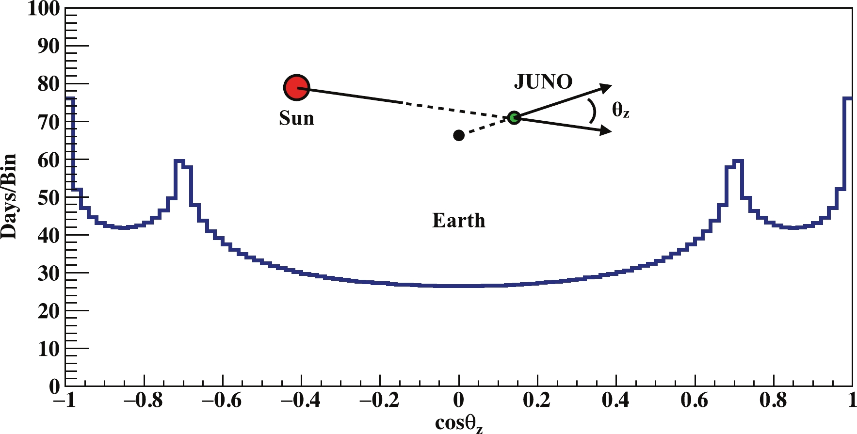
Figure 2. (color online) Definition of the solar zenith angle,
$\theta_z$ , and the effective detector exposure with respect to 1 A.U. for ten years of data acquisition.Taking the MSW effects in both the Sun and the Earth into consideration, the
$ \nu_{e} $ survival probabilities ($ P_{ee} $ ) with respect to the neutrino energy$ E_\nu $ for the two$ \Delta m^2_{21} $ values are shown in Fig. 3. The other oscillation parameters are taken from PDG-2018 [33]. The shadowed area shows the$ P_{ee} $ variation at different solar zenith angles. A transition energy region connecting the two oscillation regimes is found between 1 MeV and 8 MeV. A smooth upturn trend for$ P_{ee}(E_\nu) $ in this transition energy range is also expected. As the$ \Delta m^2_{21} $ value decreases, a steeper upturn at the transition range and a larger Day-Night asymmetry at high energies can be found. Furthermore, the$ P_{ee}(E_\nu) $ in the transition region is especially sensitive to non-standard interactions [15]. Thus, by detecting$ ^8 $ B neutrinos, the existence of new physics that sensitively affects the transition region can be tested, and the Day-Night asymmetry can be measured.
Figure 3. (color online) Solar
$\nu_{e}$ survival probabilities ($P_{ee}$ ) with respect to the neutrino energy. A transition from the MSW dominated oscillation to the vacuum dominated one is found when the neutrino energy changes from high to low ranges. The shadowed area shows the variation of$P_{ee}$ at different solar zenith angles. A smaller$\Delta m^2_{21}$ leads to a larger Day-Night asymmetry effect. -
In the
$ \nu-e $ elastic scattering process,$ \nu_{e} $ can interact with electrons via both$ W^\pm $ and$ Z^0 $ boson exchange, while$ \nu_{\mu,\tau} $ can only interact with electrons via$ Z^0 $ exchange. This leads to a cross section of$ \nu_{e} $ $ -e $ that is approximately six times larger than that of$ \nu_{\mu,\tau}-e $ , as shown in Fig. 4. For the cross section calculation, we use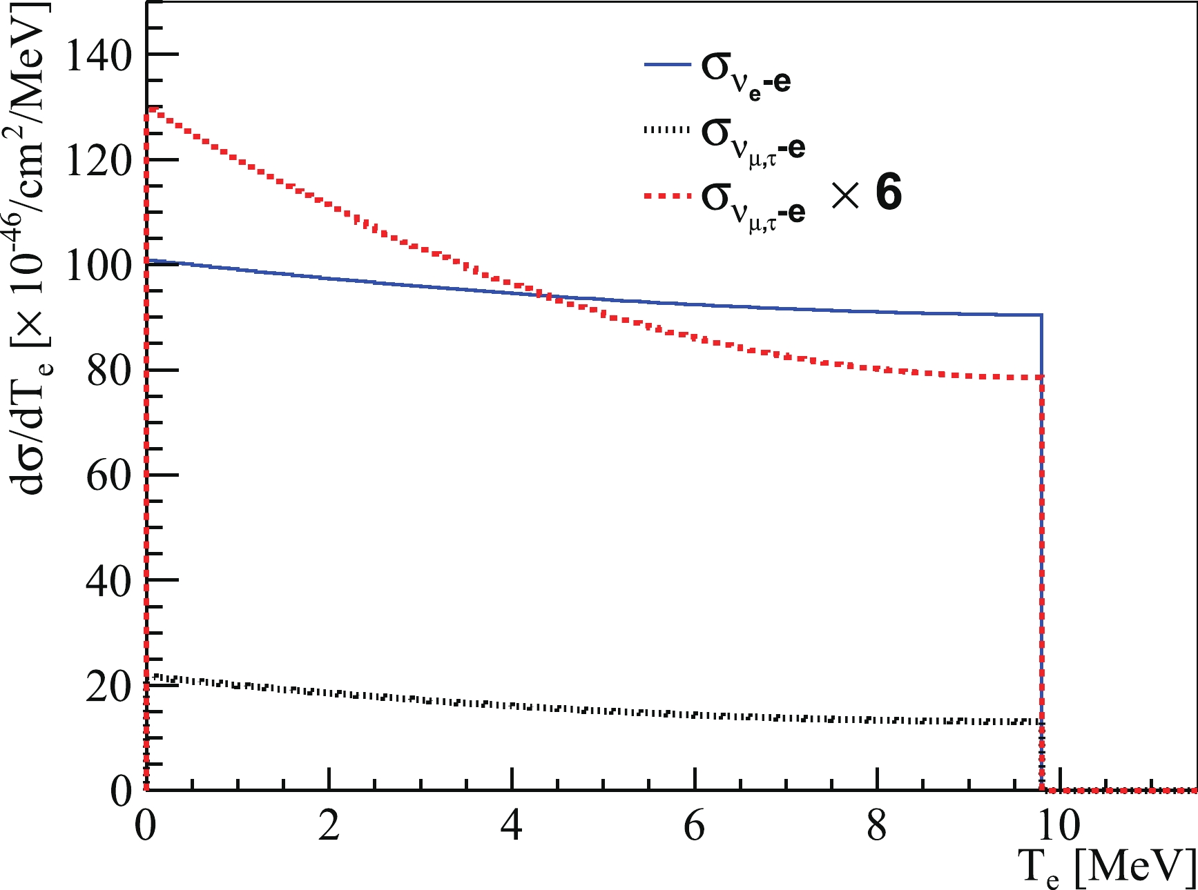
Figure 4. (color online) Differential cross section of
$\nu_e-e$ (blue) and$\nu_{\mu,\tau}-e$ (black) elastic scattering for a 10 MeV neutrino. The stronger energy dependence of the$\nu_{\mu,\tau}-e$ cross section, as illustrated in red, produces another smooth upturn in the visible electron spectrum compared with the case without the appearance of$\nu_{\mu,\tau}$ .$ \frac{{\rm d}\sigma}{{\rm d}T_e}(E_{\nu},T_e) = \frac{\sigma_0}{m_e}\left[g^2_1+g^2_2\left(1-\frac{T_e} {E_{\nu}}\right)^2-g_1g_2\frac{m_eT_e}{E_{\nu}^2}\right]\; , $

(1) where
$ E_{\nu} $ is the neutrino energy,$ T_e $ is the kinetic energy of the recoil electron,$ m_e $ is the electron mass, and$ \sigma_0 = \frac{2G^2_Fm^2_e}{\pi}\simeq88.06\times10^{-46} $ cm$ ^2 $ [34]. The quantities$ g_1 $ and$ g_2 $ depend on neutrino flavor:$ g_1^{(\nu_e)} = g_2^{(\overline{\nu}_e)}\simeq0.73 $ ,$ g_2^{(\nu_e)} = g_1^{(\overline{\nu}_e)}\simeq 0.23 $ ,$ g_1^{(\nu_{\mu,\tau})} = g_2^{(\overline{\nu}_{\mu,\tau})}\simeq-0.27 $ , and$ g_2^{(\nu_{\mu,\tau})} = g_1^{(\overline{\nu}_{\mu,\tau})}\simeq0.23 $ .After scattering, the total energy and momentum of the neutrino and electron are redistributed. Physics studies rely on the visible spectrum of recoil electrons, predicted in the following steps. First, the ES cross section is applied to the neutrino spectrum to obtain the kinetic energy spectrum of recoil electrons. To calculate the reaction rate, the electron density is 3.38
$ \times10^{32} $ per kt, using the LS composition in Ref. [22]. The expected signal rate in the full energy range is 4.15 (4.36) counts per day per kt (cpd/kt) for$ \Delta m^2_{21} $ $ = 4.8\; (7.5)\times 10^{-5} $ eV$ ^{2} $ . A simplified detector response model, including the light output nonlinearity of the LS from Daya Bay [35] and the 3%/$ \sqrt E $ energy resolution, is applied to the kinetic energy of the recoil electron, resulting in the visible energy${E}_{\rm{vis}}$ . To calculate the fiducial volumes, the ES reaction vertex is also smeared by a 12 cm/$ \sqrt E $ resolution. Eventually, the number of signals is counted with respect to the visible energy and the solar zenith angle, as shown in Fig. 5. The two-dimensional spectrum will be used to determine the neutrino oscillation parameters, as it carries information on both the spectrum distortion, primarily from oscillation in the Sun, and the Day-Night asymmetry from oscillation in the Earth. Table 1 provides the expected signal rates during Day and Night within the two visible energy ranges.Rate [cpd/kt] (0, 16) MeV (2, 16) MeV Day Night Day Night $\Delta m^2_{21}=4.8\times10^{-5}$ eV

$^2$ 

2.05 2.10 1.36 1.40 $\Delta m^2_{21}=7.5\times10^{-5}$ eV

$^2$ 

2.17 2.19 1.44 1.46 Table 1. JUNO
$^8$ B$\nu-e$ E signal rates in terms of per day per kt (cpd/kt) during the Day and Night, in different visible energy ranges.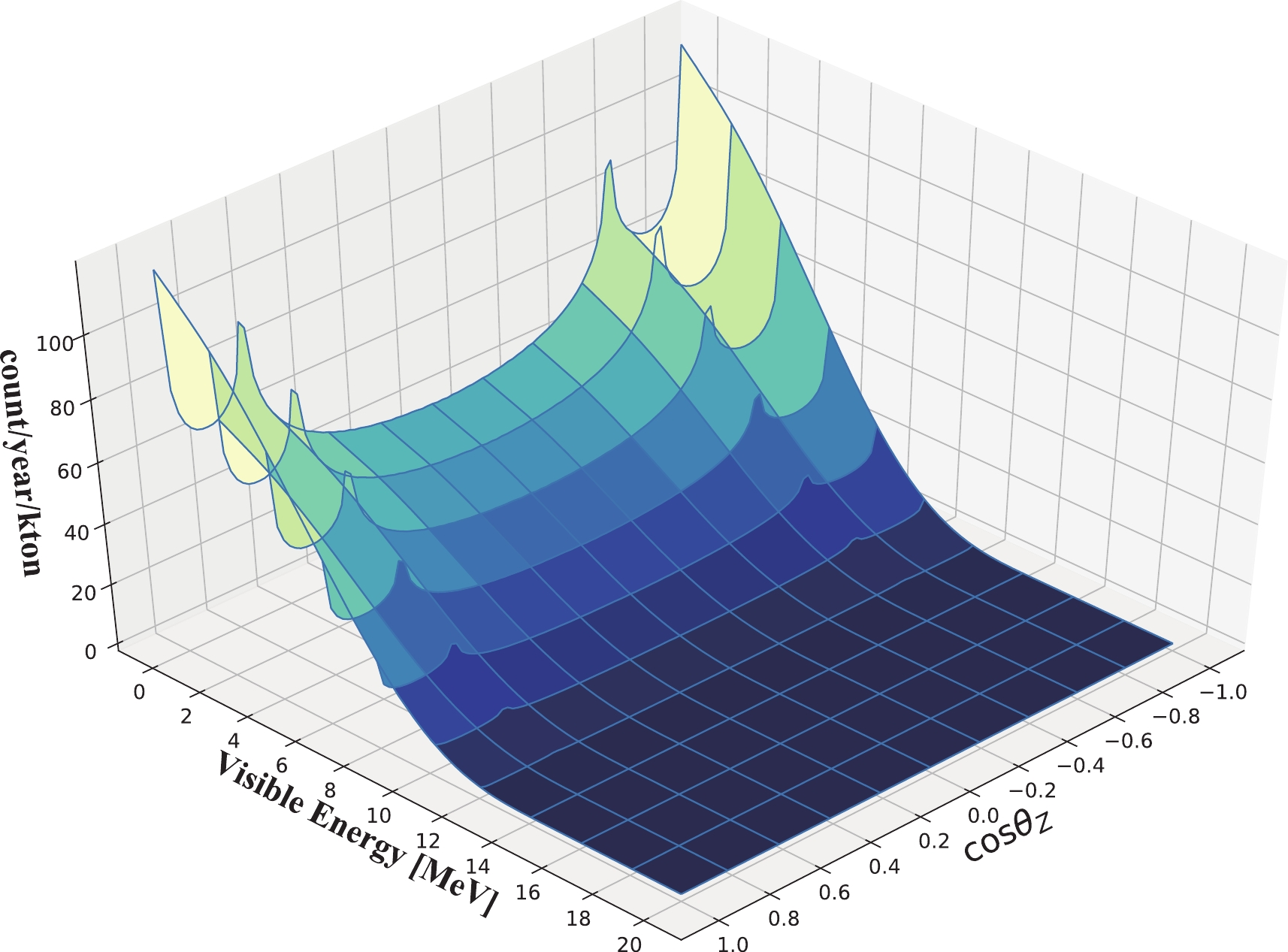
Figure 5. (color online)
$^8{\rm B}$ $\nu-e$ ES signal counts with respect to the visible energy of the recoil electron and the cosine of the solar zenith angle$\cos\theta_z$ . The spectrum carries information on neutrino oscillation both in the Sun and the Earth and can be used to determine the neutrino oscillation parameters. -
Unlike the correlated signals produced in the Inverse Beta Decay reaction of reactor antineutrinos, the ES signal of solar neutrinos corresponds to a single event. A good signal-to-background ratio requires extremely radiopure detector materials, sufficient shielding from surrounding natural radioactivity, and an effective strategy to reduce the background from unstable isotopes produced by cosmic-ray muons passing through the detector. Based on the R&D of JUNO detector components, a background budget has been built for
$ ^8 $ B neutrino detection at JUNO. Assuming an intrinsic$ ^{238} $ U and$ ^{232} $ Th radioactivity level of 10$ ^{-17} $ g/g, the 2 MeV analysis threshold can be achieved, yielding a sample from 10 years of data acquisition containing approximately 60,000 ES signal events and 30,000 background candidates.The threshold cannot be further reduced below 2 MeV because of the large background from cosmogenic
$ ^{11} $ C, which is a$ \beta^+ $ isotope with a decay energy of 1.982 MeV and a half-life of 20.4 min, with a production rate in the JUNO detector of more than 10,000 per day. The huge yield and long life-time of$ ^{11} $ C make it very difficult to suppress this background to a level similar to that of the signal, limiting the analysis threshold to 2 MeV. -
As shown in Fig. 6, the 20 kt liquid scintillator is contained in a spherical acrylic vessel with an inner diameter of 35.4 m and a thickness of 12 cm. The vessel is supported by a 600 t stainless steel (SS) structure composed of 590 SS bars connected to acrylic nodes. Each acrylic node includes an approximately 40 kg SS ring, providing sufficient strength. The LS is equipped with approximately 18,000 20-inch PMTs and 25,000 3-inch small PMTs. The 18,000 20-inch PMTs comprise 5,000 Hamamatsu dynode PMTs and 13,000 PMTs with a microchannel plate (MCP-PMT) instead of a dynode structure. All of the PMTs are installed on the SS structure, and the glass bulbs of the large PMTs are positioned approximately 1.7 m away from the LS. Pure water in the pool serves as both passive shielding and a Cherenkov muon detector equipped with approximately 2,000 20-inch PMTs. The natural radioactivity is divided into internal and external parts, where the internal part is the LS intrinsic background and the external part is from other detector components and surrounding rocks. The radioactivity of each to-be-built detector component has been measured [36] and is used in the Geant4 (10.2) based simulation [37].
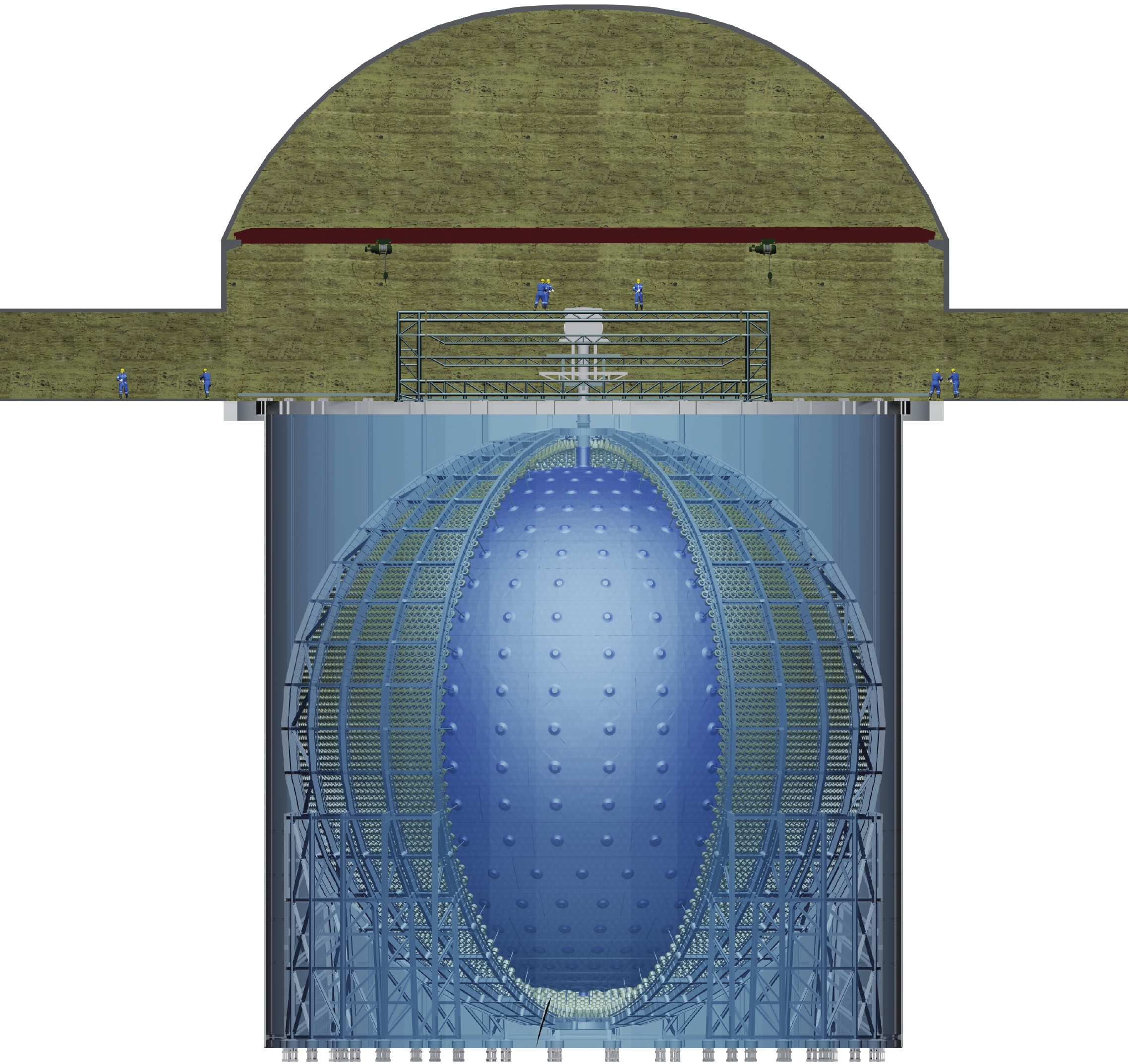
Figure 6. (color online) Diagram of the JUNO detector. The 20 kt LS is contained in a spherical acrylic vessel with an inner diameter of 35.4 m, and the vessel is supported by a stainless steel latticed shell that contains approximately 18,000 20-inch PMTs and 25,000 3-inch PMTs.
-
Among the external radioactive isotopes,
$ ^{208} $ Tl is the most critical one because it has the highest energy$ \gamma $ (2.61 MeV) from its decay. This was also the primary reason that Borexino could not lower the analysis threshold to below 3 MeV [23]. This problem is overcome in JUNO because of its much larger detector size. In addition, all detector materials at JUNO have been carefully selected to fulfill radiopurity requirements [38]. The$ ^{238} $ U and$ ^{232} $ Th contaminations in SS are measured to be less than 1 ppb and 2 ppb, respectively. In acrylic, both are at the 1 ppt level. One improvement is from the glass bulbs of MCP-PMTs, in which the$ ^{238} $ U and$ ^{232} $ Th contaminations are 200 ppb and 125 ppb, respectively [39]. These values are 2 to 4 times lower than those of the 20-inch Hamamatsu PMTs.With the measured radioactivity values, a simulation is performed to obtain the external
$ \gamma $ deposited energy spectrum in the LS, as shown in Fig. 7.$ ^{208} $ Tl decays in the PMT glass and in the SS rings of the acrylic nodes dominate the external background, which is responsible for the peak at 2.6 MeV. The continuous part from 2.6 to 3.5 MeV is due to the multiple$ \gamma $ releases from a$ ^{208} $ Tl decay. Limited by the huge computing resources required to simulate a sufficient number of$ ^{208} $ Tl decays in the PMT glass, an extrapolation method is used to estimate its contribution in the region with a spherical radius of less than 15 m, based on the simulated results in the outer region. According to the simulation results, an energy dependent fiducial volume (FV) cut, in terms of the reconstructed radial position (r) in the spherical coordinate system, is designed as follows:
Figure 7. (color online) Deposited energy spectra in LS by external
$\gamma$ after different FV cuts. The plot is generated by simulation with measured radioactivity values of all external components. The multiple$\gamma$ releases of$^{208}$ Tl decays in acrylic and SS nodes account for the background from 3 to 5 MeV. With a set of energy-dependent FV cuts, the external background is suppressed to less than 0.5% compared with the signals.● 2
$ <E_{\rm{vis}}\leqslant $ 3 MeV,$ r< $ 13 m, 7.9 kt target mass;● 3
$ <E_{\rm{vis}}\leqslant $ 5 MeV,$ r< $ 15 m, 12.2 kt target mass;●
$ E_{\rm{vis}} > $ 5 MeV,$ r< $ 16.5 m, 16.2 kt target mass.In this way, the external radioactivity background is suppressed to less than 0.5% compared with the signals in the entire energy range, while the signal statistics are maximized at high energies.
In addition to the decays of natural radioactive isotopes, another important source of high energy
$ \gamma $ is the ($ n,\; \gamma $ ) reaction in rocks, PMT glass, and the SS structure [23, 40]. Neutrons primarily come from the ($ \alpha,\; n $ ) reaction and the spontaneous fission of$ ^{238} $ U; these are denoted as radiogenic neutrons. The neutron fluxes and spectra are calculated using the neutron yields from Refs. [23, 41] and the measured radioactivity levels. Then, the simulation is performed to account for the neutron transportation and capture, high energy$ \gamma $ release, and energy deposition. In the FV of$ r< $ 16.5 m, this radiogenic neutron background contribution is found to be less than 0.001 per day and can be neglected. -
With a negligible external background after the FV cuts, the intrinsic impurity levels of the LS and backgrounds from cosmogenic isotopes determine the lower analysis threshold of recoil electrons. JUNO will deploy four LS purification approaches. Three of them focus on the removal of natural radioactivity in the LS during distillation, water extraction, and gas stripping [42]. An additional online monitoring system (OSIRIS [43]) will be built to measure the
$ ^{238} $ U,$ ^{232} $ Th, and radon contaminations before filling the LS. As a feasibility study, following the assumptions in the JUNO Yellow Book [22], we start with 10$ ^{-17} $ g/g$ ^{238} $ U and$ ^{232} $ Th in the secular equilibrium, which are close to those of Borexino Phase I [44]. However, from Borexino's measurements, the daughter nuclei of$ ^{222} $ Rn, i.e.,$ ^{210} $ Pb and$ ^{210} $ Po, are likely off-equilibrium. In this study,$ 10^{-24} $ g/g$ ^{210} $ Pb and a$ ^{210} $ Po decay rate of 2600 cpd/kt are assumed [45]. The top plot of Fig. 8 shows the internal background spectrum under the assumptions above; the$ ^8 $ B neutrino signal is also drawn for comparison. Obviously, an effective background reduction method is required. The$ \alpha $ peaks are not included because, after LS quenching, their visible energies are usually less than 1 MeV, much smaller than the 2 MeV analysis threshold.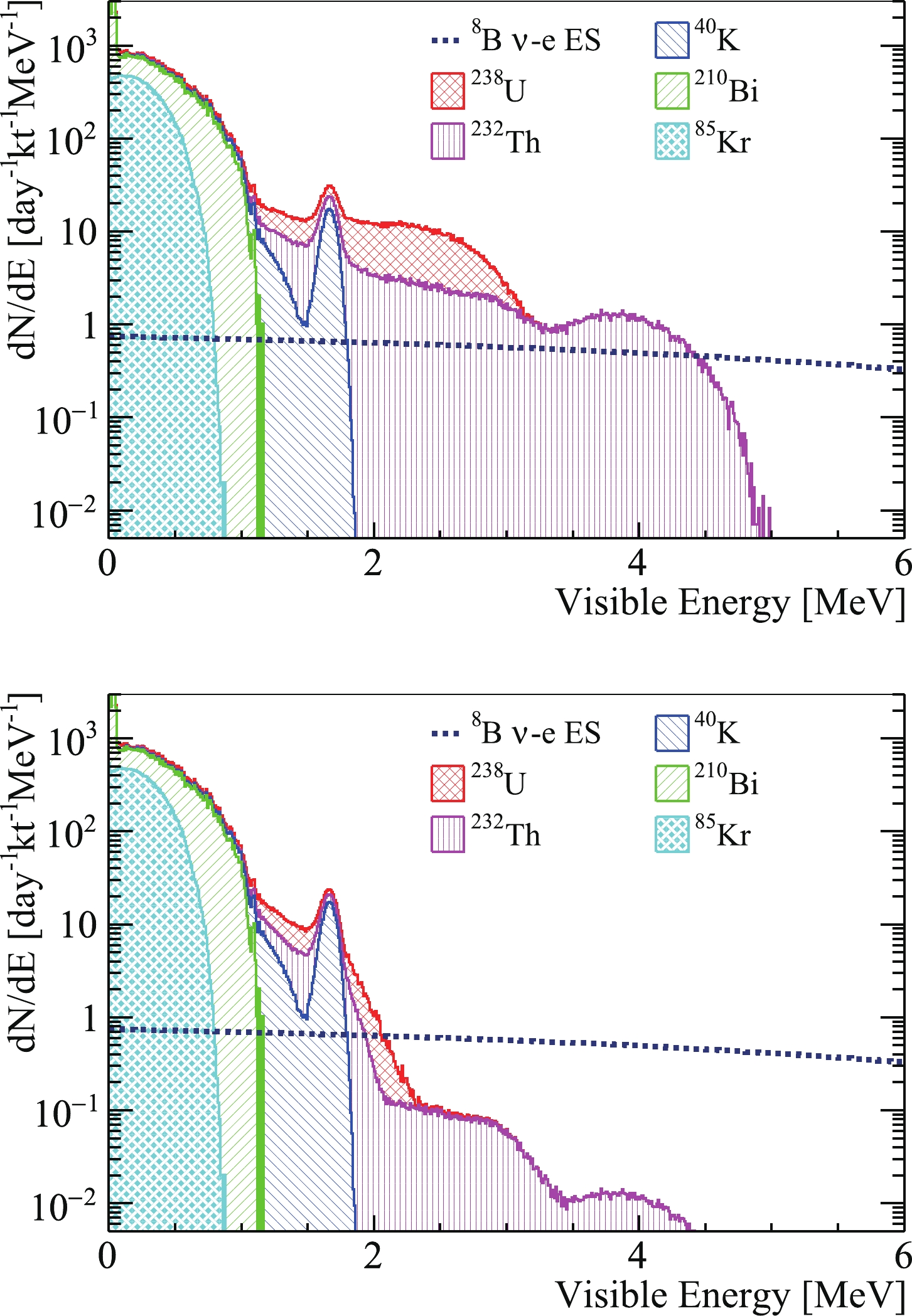
Figure 8. (color online) Internal radioactivity background compared with
$^8$ B signal before (top) and after (bottom) time, space, and energy correlation cuts to remove the Bi-Po/Bi-Tl cascade decays. The events in the$3-5$ MeV energy range are dominated by$^{208}$ Tl decays, while those between 2 and 3 MeV are from$^{214}$ Bi and$^{212}$ Bi.Above the threshold, the background is dominated by five isotopes, as listed in Table 2.
$ ^{214} $ Bi and 64% of$ ^{212} $ Bi decays can be removed by the coincidence with their short-lived daughter nuclei,$ ^{214} $ Po ($\tau\sim231\; \mu$ s) and$ ^{212} $ Po ($ \tau\sim431 $ ns), respectively. The removal efficiency of$ ^{214} $ Bi can reach approximately 99.5% with less than 1% loss of signal. Based on the current electronics design, which records PMT waveforms in a 1$\mu$ s readout window with a sampling rate of 1 G samples/s [47], it is assumed that$ ^{212} $ Po cannot be identified from its parent$ ^{212} $ Bi if it decays within 30 ns. Thus, for the$ ^{212} $ Bi-$ ^{212} $ Po cascade decays, the removal efficiency is only 93%. For the residual 7%, the visible energies of$ ^{212} $ Bi and$ ^{212} $ Po decays are added together because they are too close to each other to be considered separately.Isotope Decay mode Decay energy/MeV $\tau$ 

Daughter Daughter's $\tau$ 

Removal eff. Removed signal $^{214}$ Bi

$\beta^-$ 

3.27 28.7 min $^{214}$ Po

237 $\mu$ s

>99.5% <1% $^{212}$ Bi

$\beta^-$ : 64%

2.25 87.4 min $^{212}$ Po

431 ns 93% $\sim$ 0

$^{212}$ Bi

$\alpha$ : 36%

6.21 87.4 min $^{208}$ Tl

4.4 min N/A N/A $^{208}$ Tl

$\beta^-$ 

5.00 4.4 min $^{208}$ Pb

Stable 99% 20% $^{234}$ Pa

$^{\rm{m}}$ 

$\beta^-$ 

2.27 1.7 min $^{234}$ U

245500 years N/A N/A $^{228}$ Ac

$\beta^-$ 

2.13 8.9 h $^{228}$ Th

1.9 years N/A N/A Table 2. Isotopes in the
$^{238}$ U and$^{232}$ Th decay chains with decay energies larger than 2 MeV. With correlation cuts, most of the$^{214}$ Bi,$^{212}$ Bi, and$^{208}$ Tl decays can be removed. The decay data are taken from Ref. [46].In addition to removing
$ ^{214} $ Bi and$ ^{212} $ Bi via the prompt correlation, which was also used in previous experiments, a new analysis technique used in this study is the reduction of$ ^{208} $ Tl. 36% of$ ^{212} $ Bi decays to$ ^{208} $ Tl by releasing an$ \alpha $ particle. The decay of$ ^{208} $ Tl ($ \tau\sim $ 4.4 min) dominates the background in the energy range of 3 to 5 MeV. With a 22 min veto in a spherical volume with a radius of 1.1 m around a$ ^{212} $ Bi$ \alpha $ candidate, 99% of$ ^{208} $ Tl decays can be removed. The fraction of removed good events, estimated with the simulation, is found to be approximately 20% because there are more than 2600 cpd/kt$ ^{210} $ Po decays in the similar$ \alpha $ energy range. Eventually, the signal over background (S/B) ratio in the energy range of$ 3-5 $ MeV is significantly improved, from 0.6 to 35.However, for
$ ^{228} $ Ac and$ ^{234} $ Pa$ ^{\rm{m}} $ , both of which have decay energies slightly larger than 2 MeV, there are no available cascade decays for background elimination. If the$ ^{238} $ U and$ ^{232} $ Th decay chains are in secular equilibrium, their contributions can be statistically subtracted with the measured Bi-Po decay rates. Otherwise, the analysis threshold will increase to approximately 2.3 MeV.Considering higher radioactivity level assumptions, if the
$ ^{238} $ U and$ ^{232} $ Th contaminations are$ 10^{-16} $ g/g, the 2 MeV threshold is still achievable but with a worse S/B ratio in the energy range of 3 to 5 MeV. A$ 10^{-15} $ g/g contamination would result in a 5 MeV analysis threshold, determined by the end-point energy of$ ^{208} $ Tl decay. If$ ^{238} $ U and$ ^{232} $ Th contaminations reach to$ 10^{-17} $ g/g, but the$ ^{210} $ Po decay rate is greater than 10,000 cpt/kt, as in Borexino Phase I [44], the$ ^{208} $ Tl reduction mentioned above cannot be performed. Consequently, the$ ^{208} $ Tl background can only be statistically subtracted. The influence of these radioactivity level assumptions on the neutrino oscillation studies will be discussed in Sec. IVC. -
In addition to natural radioactivity, another crucial background source comes from the decay of light isotopes produced by the cosmic-ray muon spallation process in the LS. The relatively shallow vertical rock overburden, approximately 680 m, leads to a 0.0037 Hz/m
$ ^2 $ muon flux, with an averaged energy of 209 GeV. The direct consequence is approximately 3.6 Hz muons passing through the LS target. More than 10,000$ ^{11} $ C isotopes are generated per day, which constrains the analysis threshold to 2 MeV, as shown in Fig. 9. Based on the simulation and measurements of previous experiments, it is found that other isotopes can be suppressed to a 1% level with a cylindrical veto along the muon track and the Three-Fold Coincidence cut (TFC) among the muon, the spallation neutron capture, and the isotope decay [50, 51]. Details are presented in this section.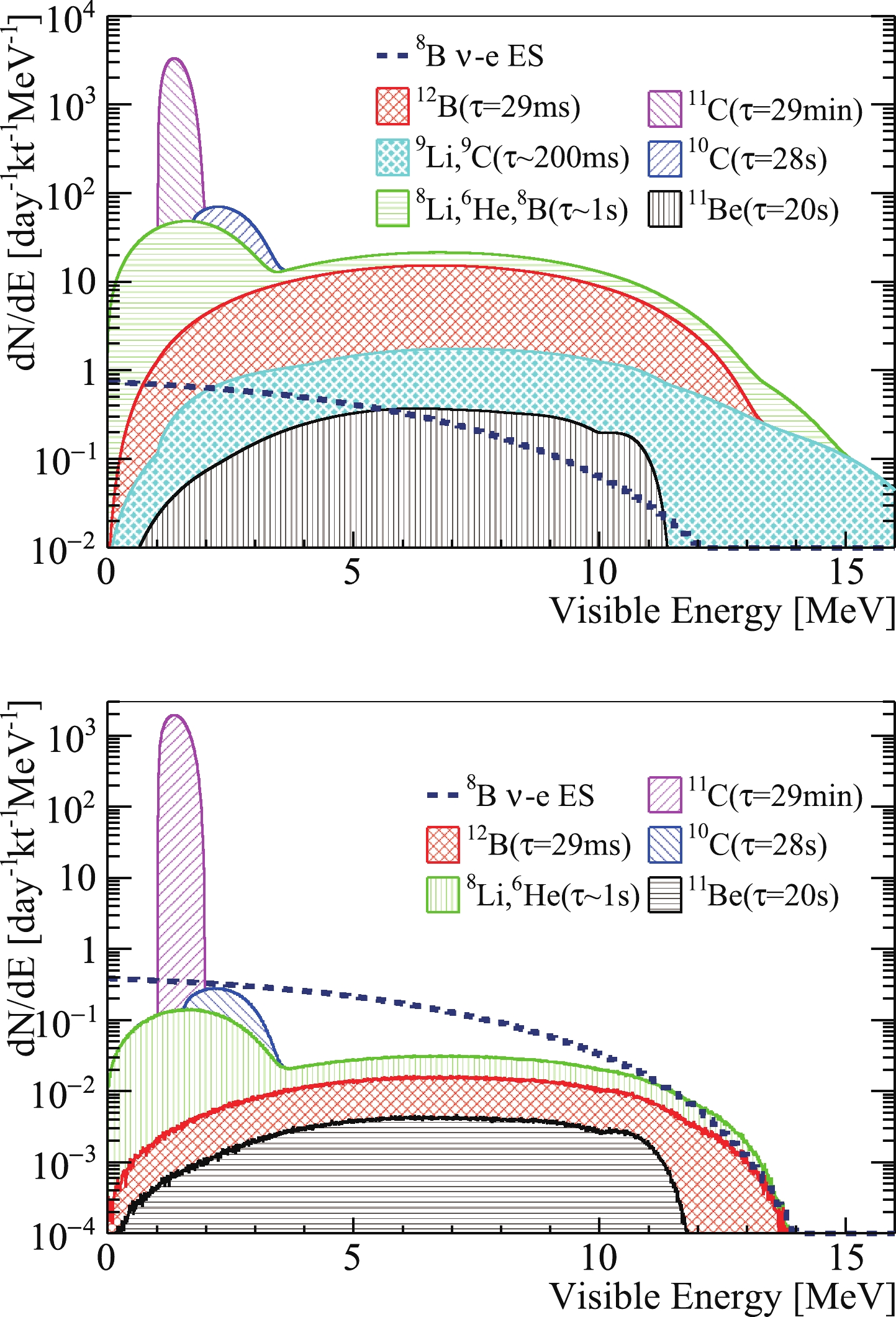
Figure 9. (color online) Cosmogenic background before (top) and after veto (bottom). The isotope yields shown here are scaled from KamLAND [48] and Borexino measurements [49]. The huge amount of
$^{11}$ C constrains the analysis threshold to 2 MeV. The other isotopes can be well suppressed with veto strategies discussed in the text. -
When a muon passes through the LS, along with the ionization, many secondary particles are also generated, including
$ e^\pm $ ,$ \gamma $ ,$ \pi^{\pm} $ , and$ \pi^{\rm{0}} $ . Neutrons and isotopes are produced primarily via the ($ \gamma $ , n) and$ \pi $ inelastic scattering processes. More daughters could come from the neutron inelastic scattering on carbon. Such a process is defined as a hadronic shower, in which most of the cosmogenic neutrons and light isotopes are generated. More discussion on the muon shower process can be found in Refs. [52, 53]. To understand the shower physics and develop a reasonable veto strategy, a detailed muon simulation has been carried out. The simulation starts with CORSIKA [54] for the cosmic air shower simulation at the JUNO site, which gives the muon energy, momentum, and multiplicity distribution arriving at the surface. Then, MUSIC [55] is employed to track muons traversing the rock to the underground experiment hall, based on the local geological map. The muon sample after transportation is used as the event generator for Geant4, with which the detector simulation is performed and all secondary particles are recorded. A simulation data set consisting of 16 million muon events is prepared, corresponding to approximately 50 days of statistics.In the simulation, the average muon track length in the LS is approximately 23 m, and the average deposited energy via ionization is 4.0 GeV. Given the huge detector size, approximately 92% of the 3.6 Hz LS muon events consist of one muon track, 6% have two muon tracks, and the rest have more than two. Events with more than one muon track are called muon bundles. In general, all of the muon tracks in one bundle are from the same air shower and are parallel to each other. In more than 85% of the bundles, the distance between muon tracks is larger than 3 m.
The cosmogenic isotopes affecting this analysis are listed in Table 3. The simulated isotope yields are found to be lower than those measured by KamLAND [48] and Borexino [49]. Thus, in our background estimation, the yields are scaled to the results of the two experiments, by empirically modelling the production cross section as being proportional to
$ E_\mu^{0.74} $ , where$ E_\mu $ is the average energy of the muon at the detector. Because the$ \gamma $ ,$ \pi $ , and neutron mean free paths in the LS are tens of centimeters, the generation positions of the isotopes are close to the muon track, as shown in Fig. 10. For more than 97% of the isotopes, the distances are less than 3 m, leading to an effective cylindrical veto along the reconstructed muon track. However, the veto time can only be set to 3 to 5 s to keep a reasonable detector live time, which removes a small fraction of$ ^{11} $ C and$ ^{10} $ C. Thus, as mentioned before, the$ ^{11} $ C, primarily from the$ ^{12} $ C ($ \gamma,\; n $ ) reaction, with the largest yield and a long life time, will push the analysis threshold of the recoil electron to 2 MeV. The removal of$ ^{10} $ C, primarily generated in the$ ^{12} $ C ($ \pi^+,\; np $ ) reaction, relies on the TFC among the muon, neutron capture, and isotope decay.Isotope Decay mode Decay energy/MeV $\tau$ 

Yield in LS (/day) TFC fraction Geant4 simulation Scaled $^{12}$ B

$\beta^-$ 

13.4 29.1 ms 1059 2282 90% $^{9}$ Li

$\beta^-$ : 50%

13.6 257.2 ms 68 117 96% $^{9}$ C

$\beta^+$ 

16.5 182.5 ms 21 160 >99% $^{8}$ Li

$\beta^-+\alpha$ 

16.0 1.21 s 725 649 94% $^{6}$ He

$\beta^-$ 

3.5 1.16 s 526 2185 95% $^{8}$ B

$\beta^++\alpha$ 

$\sim$ 18

1.11 s 35 447 >99% $^{10}$ C

$\beta^+$ 

3.6 27.8 s 816 878 >99% $^{11}$ Be

$\beta^-$ 

11.5 19.9 s 9 59 96% $^{11}$ C

$\beta^+$ 

1.98 29.4 min 11811 46065 98% Table 3. Summary of cosmogenic isotopes in JUNO. The isotope yields extracted from the Geant4 simulation, as well as the ones scaled to the measurements, are listed. The TFC fraction denotes the probability of finding at least one spallation neutron capture event between the muon and the isotope decay.
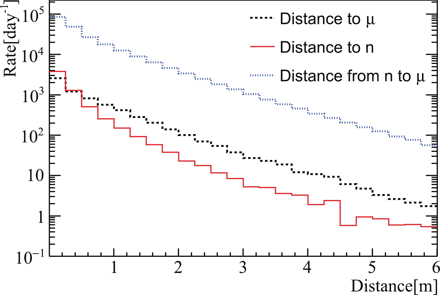
Figure 10. (color online) Distribution of the simulated distance between an isotope and its parent muon track (black), and the distance between the isotope and the closest spallation neutron candidate (red). The distance between a spallation neutron capture and its parent muon is shown in blue.
To perform the cylindrical volume veto, muon track reconstruction is required. There have been several reconstruction algorithms developed for JUNO, as reported in Refs. [56-59]. A precision muon reconstruction algorithm was also developed in Double Chooz [60]. Based on these studies, the muon reconstruction strategy in JUNO is assumed to be as follows. 1) If there is only one muon in the event, the track can be well reconstructed. 2) If there are two muons with a distance larger than 3 m in one event, which contributes to 5.5% of the total events, the two muons can be recognized and both are well reconstructed. If the distance is less than 3 m (0.5%), the number of muons can be identified via the energy deposit, but only one track can be reconstructed. 3) If there are more than two muons in one event (2%), it is conservatively assumed that no track information can be extracted, and the whole detector will be vetoed for 1 s. 4) If the energy deposit is larger than 100 GeV (0.1%), no matter how many muons are in the event, it is assumed that no track can be reconstructed from such a big shower.
To design the TFC veto, the characteristics of neutron production are obtained from the simulation. Approximately 6% of single muons and 18% of muon bundles produce neutrons, and the average numbers of neutrons are approximately 11 and 15, respectively. Most of the neutrons are close to each other, forming a spherical volume with a high concentration of neutrons. This volume can be used to estimate the shower position. The simulated neutron yields are compared with the data of several experiments, such as Daya Bay [61], KamLAND [48], and Borexino [62]. The differences are found to be less than 20%. The spatial distributions of the neutrons, defined as the distance between the neutron capture position and its parent muon track, are shown in Fig. 10. More than 90% of the neutrons are captured within 3 m from the muon track, consistent with KamLAND's measurement. The advantage of LS detectors is the high detection efficiency of the neutron capture for hydrogen and carbon, which can be as high as 99%. If there is at least one neutron capture between the muon and the isotope decay, the event is defined as TFC tagged. Then, the TFC fraction is the ratio of the number of tagged isotopes to the total number of generated isotopes. In Table 3, the TFC fraction in the simulation is summarized. The high TFC fraction comes from two aspects: the first is that a neutron and an isotope are simultaneously produced, such as
$ ^{11} $ C and$ ^{10} $ C. The other one is the coincidence between one isotope and the neutron(s) generated in the same shower. If one isotope is produced, the median of neutrons generated by this muon is 13, and for more than one isotope, the number of neutrons increases to 110, as isotopes are usually generated in showers with large energy deposits. The red line in Fig. 10 shows the distance between an isotope decay and the nearest neutron capture, which is mostly less than 2 m. -
Based on the information above, the muon veto strategy is designed as follows.
● Whole detector veto:
Veto 2 ms after every muon event, passing through either the LS or water;
Veto 1 s for muon events without reconstructed tracks.
● The cylindrical volume veto, depending on the distance (d) between the candidate and the muon track:
Veto
$ d< $ 1 m for 5 s;Veto 1 m
$ <d< $ 3 m for 4 s;Veto 3 m
$ <d< $ 4 m for 2 s;Veto 4 m
$ <d< $ 5 m for 0.2 s.● The TFC veto:
Veto a 2 m spherical volume around a spallation neutron candidate for 160 s.
In the cylindrical volume veto, the 5 s and 4 s veto times are determined based on the life of
$ ^8 $ B and$ ^{8} $ Li. The volume with d between 4 and 5 m is mostly to remove$ ^{12} $ B, which has a larger average distance because the primary generation process is$ ^{12} $ C($ n,p $ ), and neutrons have a larger mean free path than$ \gamma $ 's and$ \pi $ 's. For muon bundles with two muon tracks reconstructed, the above cylindrical volume veto will be applied to each track. Compared with the veto strategies that reject any signal within a time window of 1.2 s and a 3 m cylinder along the muon track [22, 63], the above distance-dependent veto significantly improves the S/B ratio. The TFC veto is designed for the removal of$ ^{10} $ C and$ ^{11} $ Be. Moreover, it effectively removes$ ^8 $ B,$ ^{8} $ Li, and$ ^{6} $ He generated in large showers and muon bundles without track reconstruction abilities.The muons not passing through LS, defined as external muons, contribute to approximately 2% of isotopes, concentrated at the edge of the LS. Although there is no available muon track for background suppression, the FV cut can effectively eliminate these isotopes and reach a B/S ratio of less than 0.1%, which can be safely neglected.
To estimate the dead time induced by the veto strategy and the residual background, a toy Monte Carlo sample is generated by mixing the
$ ^8 $ B neutrino signal with the simulated muon data. The whole detector veto and the cylindrical volume veto introduce 44% dead time, while the TFC veto adds an additional 4%. The residual backgrounds above the 2 MeV analysis threshold consist of$ ^{12} $ B,$ ^8 $ Li,$ ^6 $ He,$ ^{10} $ C, and$ ^{11} $ Be, as shown in Fig. 9. A potential improvement on the veto strategy may come from a joint likelihood based on the muon energy deposit density, the number of spallation neutrons, and time and distance distributions between the isotope and muon and those among the isotope and neutrons. In addition, this study could profit from the developing topological method for discrimination between the signal ($ e^- $ ) and background ($ ^{10} $ C,$ e^++\gamma $ ) [56].The actual isotope yields, distance distributions, and TFC fractions will be measured
$ in $ -$ situ $ in the future. Estimation of residual backgrounds and uncertainties will rely on these measurements. Currently, the systematic uncertainties are assumed based on KamLAND's measurements [40], given the comparable overburden (680 m and 1000 m): 1% uncertainty for$ ^{12} $ B, 3% uncertainty for$ ^8 $ Li and$ ^6 $ He, and 10% uncertainty for$ ^{10} $ C and$ ^{11} $ Be. -
The reactor antineutrino flux at the JUNO site is approximately
$ 2\times10^7 $ /cm$ ^2 $ /s, assuming 36 GW of thermal power. Combining the oscillated antineutrino flux with the corresponding cross section [64], the inverse beta decay (IBD) reaction rate between$ \overline{\nu}_{e} $ and protons is approximately 4 cpd/kt, and the elastic scattering rate between$ \overline{\nu}_{x} $ and electrons is approximately 1.9 cpd/kt in the energy range of 0 to 10 MeV. The products of the IBD reaction,$ e^+ $ and neutron, can be rejected to less than 0.5% using the correlation between them. The residual primarily comes from the two signals falling into one electronics readout window (1$\mu$ s). The recoil electron from the$ \overline{\nu}-e $ ES channel, with a rate of 0.14 cpd/kt when the visible energy is greater than 2 MeV, cannot be distinguished from$ ^8 $ B$ \nu $ signals. A 2% uncertainty is assigned to this background, according to the uncertainties of antineutrino flux and the ES cross section. -
After applying all the selection cuts, approximately 60,000 recoil electrons and 30,000 background events are expected in 10 years of data acquisition, as listed in Table 4 and shown in Fig. 11. The dead time resulting from the muon veto is approximately 48% in the whole energy range. As listed in Table 2, the
$ ^{212} $ Bi$ - $ $ ^{208} $ Tl correlation cut removes 20% of signals in the energy range of 3 to 5 MeV and less than 2% in other energy ranges. The detection efficiency uncertainty, primarily from the FV cuts, is assumed to be 1%, according to Borexino's results [23]. Given that the uncertainty of the FV is determined using the uniformly distributed cosmogenic isotopes, the uncertainty is assumed to be correlated among the three energy-dependent FVs. Because a spectrum distortion test will be performed, another important uncertainty source is the detector energy scale. For electrons with energies larger than 2 MeV, the nonlinear relationship between the LS light output and the deposited energy is less than 1%. Moreover, electrons from the cosmogenic$ ^{12} $ B decays, with an average energy of 6.4 MeV, can set strong constraints on the energy scale, as was done at Daya Bay [35] and Double Chooz [65]. Thus, a 0.3% energy scale uncertainty is used in this analysis, following the results in Ref. [35]. Three analyses are reported based on these inputs.cpd/kt FV $ ^8 $ B signal eff.

$ ^{12} $ B

$ ^{8} $ Li

$ ^{10} $ C

$ ^{6} $ He

$ ^{11} $ Be

$ ^{238} $ U

$ ^{232} $ Th

$ \overline{\nu} $ -e ES

Total bkg. Signal rate at $ \Delta m^{2\star}_{21} $ 

$ \Delta m^{2\dagger}_{21} $ 

(2, 3) MeV 7.9 kt $ \sim $ 51%

0.005 0.006 0.141 0.084 0.002 0.050 0.050 0.049 0.39 0.32 0.30 (3, 5) MeV 12.2 kt $ \sim $ 41%

0.013 0.018 0.014 0.008 0.005 0 0.012 0.016 0.09 0.42 0.39 (5, 16) MeV 16.2 kt $ \sim $ 52%

0.065 0.085 0 0 0.023 0 0 0.002 0.17 0.61 0.59 Syst. error 1% $ < $ 1%

3% 10% 3% 10% 1% 1% 2% Table 4. Summary of signal and background rates in different visible energy ranges with all selection cuts and muon veto methods applied.
$ \Delta m^{2\star}_{21} $ =$ 4.8\times10^{-5} $ eV$ ^2 $ and$ \Delta m^{2\dagger}_{21} $ =$ 7.5\times10^{-5} $ eV$ ^2 $ 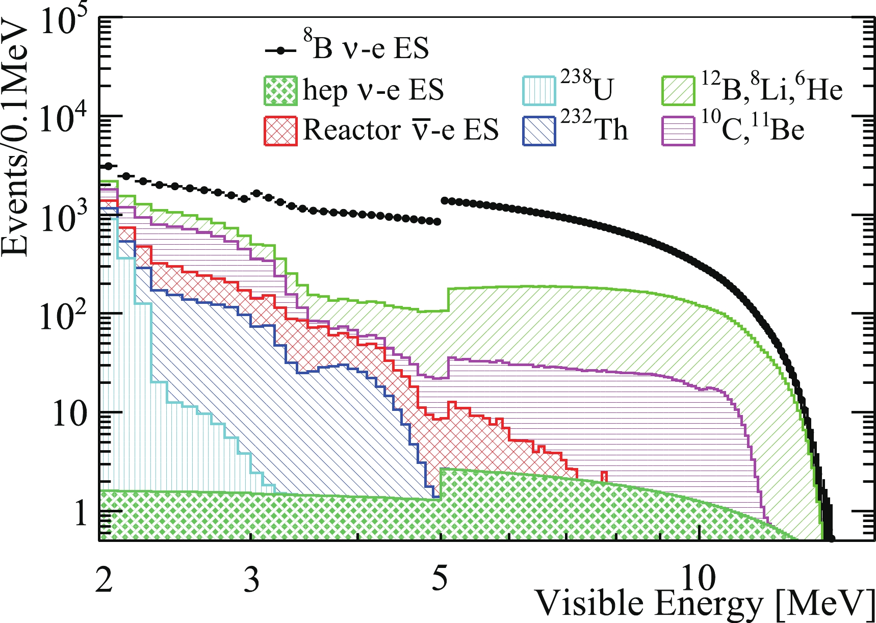
Figure 11. (color online) Expected signal and background spectra in ten years of data acquisition, with all selection cuts and muon veto methods applied. Signals are produced in the standard LMA-MSW framework using
$\Delta m^2_{21}$ =$4.8\times10^{-5}$ eV$^2$ . The energy dependent fiducial volumes account for the discontinuities at 3 MeV and 5 MeV. -
In the observed spectrum, the upturn comes from two aspects: the presence of
$ \nu_{\mu,\tau} $ and the upturn in$ P_{ee} $ . A background-subtracted Asimov data set is produced in the standard LMA-MSW framework using$ \Delta m^2_{21} $ =$ 4.8\times10^{-5} $ eV$ ^2 $ , shown as the black points in the top panel of Fig. 12. The other oscillation parameters are taken from PDG 2018 [33]. The error bars show only the statistical uncertainties. The ratio to the prediction of no-oscillation is shown as the black points in the bottom panel of Fig. 12. Here, no-oscillation is defined as pure$ \nu_{e} $ with an arrival flux of 5.25$ \times10^6 $ /cm$ ^2 $ /s. The signal rate variation with respect to the solar zenith angle has been averaged. The expected signal spectrum using$ \Delta m^2_{21} $ =$ 7.5\times10^{-5} $ eV$ ^2 $ is also plotted as the red line for comparison. More signals can be found in the low energy range. The spectral difference provides the sensitivity that enables measurement of$ \Delta m^2_{21} $ .
Figure 12. (color online) Background subtracted spectra produced in the standard LMA-MSW framework for two
$\Delta m^2_{21}$ values (black dots and red line, respectively) and the$P_{ee}=0.32 (E_\nu>2 \;{\rm{MeV}})$ assumption (blue line). Their comparison with the no flavor conversion is shown in the bottom panel. Only statistical uncertainties are shown. Details can be found in the text.First, we would like to test an energy-independent hypothesis, where
$ P_{ee} $ is assumed to be a flat value for neutrino energies larger than 2 MeV. An example spectrum generated with$ P_{ee} = 0.32 $ is plotted as the blue line in Fig. 12. Comparing with the no-oscillation prediction, the upturn of the blue line comes from the appearance of$ \nu_{\mu,\tau} $ s, which have a different energy dependence in the$ \nu-e $ ES cross section, as shown in Fig. 4. To quantify the sensitivity of rejecting this hypothesis, a$ \chi^2 $ statistic is constructed as follows:$ \begin{aligned}[b] \chi^2 =& 2\times\sum\limits_{i = 1}^{140}\left(N^i_{\rm pre}-N^i_{\rm obs}+N^i_{\rm obs}\times \log\frac{N^i_{\rm obs}}{N^i_{\rm pre}}\right) +\left(\frac{\varepsilon_d}{\sigma_d}\right)^2\\&+\left(\frac{\varepsilon_f}{\sigma_f}\right)^2+\left(\frac{\varepsilon_s}{\sigma_s}\right)^2+\left(\frac{\varepsilon_e}{\sigma_e}\right)^2+\sum\limits_{j = 1}^{10}\left(\frac{\varepsilon^j_b}{\sigma^j_b}\right)^2 , \\ N^i_{\rm pre} =& \left(1+\varepsilon_d+\varepsilon_f+\alpha^i\times\varepsilon_s + \beta^i\times\frac{\varepsilon_e}{0.3\%}\right)\times T_i \\&+ \sum\limits_{j = 1}^{10} (1+\varepsilon^j_b)\times B_{ij}, \end{aligned} $

(2) where
$N^i_{\rm obs}$ is the observed number of events in the$i^{\rm th}$ energy bin in the LMA-MSW framework;$N^i_{\rm pre}$ is the predicted one in this energy bin, by adding the signal$ T_i $ generated under the flat$ P_{ee} $ hypothesis with the backgrounds$ B_{ij} $ , which is summed over j. Systematic uncertainties are summarized in Table 5. The detection efficiency uncertainty is$ \sigma_d $ (1%), the neutrino flux uncertainty is$ \sigma_f $ (3.8%), and$ \sigma^j_b $ is the uncertainty of the$j^{\rm th}$ background, summarized in Table 4. The corresponding nuisance parameters are$ \varepsilon_d $ ,$ \varepsilon_f $ , and$ \varepsilon^j_b $ , respectively.Table 5. Summary of the systematic uncertainties. Because the uncertainty of the
$^8$ B$\nu$ spectrum shape is absorbed in the coefficients$\alpha^i$ ,$\sigma_s$ is equal to 1. See the text for details.The two uncertainties relating to the spectrum shape, the
$ ^8 $ B$ \nu $ spectrum shape uncertainty$ \sigma_s $ and the detector energy scale uncertainty$ \sigma_e $ , are implemented in the statistic using the coefficients$ \alpha^i $ and$ \beta^i $ , respectively. The neutrino energy spectrum with 1$ \sigma $ deviation is converted to the visible spectrum of the recoil electron. Its ratio to the visible spectrum converted from the nominal neutrino spectrum is denoted as$ \alpha^i $ . In this way, the corresponding nuisance parameter,$ \varepsilon_s $ , follows the standard Gaussian distribution. For the 0.3% energy scale uncertainty,$ \beta^i $ is derived from the ratio of the electron visible spectrum shifted by 0.3% to the visible spectrum without shifting.By minimizing
$ \chi^2 $ , the probabilities of excluding the flat$ P_{ee}(E_\nu $ $ > $ $ 2\; {\rm{MeV}}) $ hypothesis, in terms of$ \Delta \chi^2 $ values, are listed in Table 6. The total neutrino flux is constrained with a 3.8% uncertainty ($ \sigma_f $ ) from the SNO NC measurement, while the$ P_{ee} $ value is free in the minimization. The sensitivity is higher at larger$ \Delta m^2_{21} $ values because of the larger upturn in the visible energy spectrum. If the true$ \Delta m^2_{21} $ value is$ 7.5\times10^{-5} $ eV$ ^2 $ , the hypothesis could be rejected at the 2.7$ \sigma $ level. The statistics-only sensitivity of rejecting the flat$ P_{ee} $ hypothesis is$ \Delta \chi^2 = 4.9 $ (18.9) for$ \Delta m^2_{21} = 4.8 \times 10^{-5} $ eV$ ^2 $ ($ 7.5 \times 10^{-5} $ eV$ ^2 $ ) for the 3 MeV threshold, compared with$ \Delta \chi^2 = 7.1 $ (24.9) for the 2 MeV threshold.$\Delta \chi^2$ 

$4.8\times10^{-5}$ eV

$^2$ 

$7.5\times10^{-5}$ eV

$^2$ 

Stat. only 7.1 24.9 Stat. + $^8$ B flux error

6.8 24.2 Stat. + $^8$ B shape error

3.6 11.8 Stat. + energy scale error 4.7 15.5 Stat. + background error 3.6 14.0 Final 2.0 7.3 Table 6. Rejection sensitivity for the flat
$P_{ee}(E_\nu$ $>$ $2 \;{\rm{MeV}})$ hypothesis with 10 years of data acquisition for the two$\Delta m^2_{21}$ values. The impact of each systematic uncertainty is also listed separately.To understand the effect of systematics, the impact of each systematic uncertainty is also provided in Table 6. The sensitivity is significantly reduced after introducing the systematics. For instance, with
$ \Delta m^2_{21} $ =$ 7.5\times10^{-5} $ eV$ ^2 $ , including the neutrino spectrum shape uncertainty ($ \sigma_s $ ) almost halves the sensitivity because the shape uncertainty can affect the ratio of events in the high and low visible energy ranges. If the detector energy scale uncertainty ($ \sigma_e $ ) is included, the sensitivity is also significantly reduced for the same reason. -
Solar neutrino propagation through the Earth is expected, via the MSW effect, to cause signal rate variation versus the solar zenith angle. This rate variation observable also provides additional sensitivity to the
$ \Delta m^2_{21} $ value, as shown in Fig. 13. The blue and red dashed lines represent the average ratio of the measured signal to the no-oscillation prediction, and they are calculated with$ \Delta m^2_{21} $ =$ 4.8\times10^{-5} $ eV$ ^2 $ and$ 7.5\times10^{-5} $ eV$ ^2 $ , respectively. The solid lines show the signal rate variations versus solar zenith angle. Smaller$ \Delta m^2_{21} $ values result in a larger MSW effect in the Earth and increased Day-Night asymmetry. The error bars are the expected uncertainties.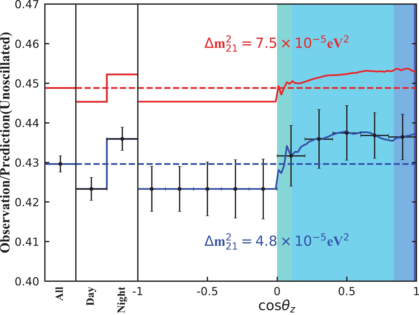
Figure 13. (color online) Ratio of
$^8$ B neutrino signals produced in the standard LMA-MSW framework to the no-oscillation prediction at different solar zenith angles. The uncertainties are propagated with a toy Monte Carlo simulation, and most of the systematic uncertainties are cancelled.The variation is quantified by defining the Day-Night asymmetry as follows:
$ A_{\rm DN} = \frac{R_{\rm D}-R_{\rm N}}{(R_{\rm D}+R_{\rm N})/2}, $

(3) where
$R_{\rm D}$ and$R_{\rm N}$ are the background-subtracted signal rates during the Day ($ \cos\theta_z<0 $ ) and Night ($ \cos\theta_z>0 $ ), respectively. They are obtained by dividing the signal numbers listed in Table 7 by the effective exposure in Fig. 2. The uncertainties are propagated with a toy Monte Carlo program to correctly include the correlation among systematics. With ten years of data acquisition, JUNO has the potential to observe the Day-Night asymmetry at a significance of 3$ \sigma $ if$ \Delta m^2_{21} $ =$ 4.8\times10^{-5} $ eV$ ^2 $ . Even when restricted to an energy range from 5 to 16 MeV, within which neither natural radioactivity nor$ ^{10} $ C are significant, a 2.8$ \sigma $ significance can still be achieved. If$ \Delta m^2_{21} $ =$ 7.5\times10^{-5} $ eV$ ^2 $ , the expected$A_{\rm DN}$ is$ (-1.6\pm0.9) $ % for the 2 to 16 MeV energy range. The different$ A_{DN} $ values also contribute to the$ \Delta m^2_{21} $ determination.Energy Exposure Day Night $A_{\rm DN}$ 

2 $\sim$ 3 MeV

41 kt $\cdot$ y

4334 4428 (-2.1 $\pm$ 3.2)%

3 $\sim$ 5 MeV

51 kt $\cdot$ y

8686 8906 (-2.5 $\pm$ 1.7)%

5 $\sim$ 16 MeV

84 kt $\cdot$ y

17058 17644 (-3.4 $\pm$ 1.2)%

2 $\sim$ 16 MeV

N/A 30078 30977 (-2.9 $\pm$ 0.9)%

Table 7. Number of background-subtracted signals during Day and Night in ten years of data acquisition for
$\Delta m^2_{21}$ =$4.8\times10^{-5}$ eV$^2$ . A set of energy-dependent FV cuts is used, and the values of the three energy ranges are provided. The uncertainties are dominated by signal and background statistics.The
$A_{\rm DN}$ measurement uncertainty is dominated by statistics because most of the systematic uncertainties are cancelled in the numerator and denominator. Potential systematics could arise from differences in detector performance during Day and Night; however, this is expected to be negligible for the LS detector. Compared with Super-Kamiokande's results from Ref. [19], JUNO could reach the same precision of$A_{\rm DN}$ in less than 10 years. The primary improvement is a better S/B ratio, as JUNO can reject$ ^{208} $ Tl via the$ \alpha $ -$ \beta $ cascade decay and suppress cosmogenic isotopes via the TFC technique. -
As mentioned above, in the standard neutrino oscillation framework,
$ \Delta m^2_{21} $ can be measured using the information in the spectra distortion and the signal rate variation versus solar zenith angle. The signal rate versus visible energy and zenith angle ($ \cos\theta_z $ ) is illustrated in Fig. 5. To fit the distribution, a$ \chi^2 $ statistic is defined as follows:$ \begin{aligned}[b] \chi^2 =& 2 \times\sum\limits_{i = 1}^{140}\sum\limits_{j = 1}^{100} \left\{ N^{\rm pre}_{i,j} - N^{\rm obs}_{i,j} + N^{\rm obs}_{i,j} \log \frac{ N^{\rm obs}_{i,j}}{ N^{\rm pre}_{i,j} } \right\} \\ & + \left(\frac{\varepsilon_d}{\sigma_d}\right)^2+\left(\frac{\varepsilon_f}{\sigma_f}\right)^2+\left(\frac{\varepsilon_s}{\sigma_s}\right)^2+\left(\frac{\varepsilon_e}{\sigma_e}\right)^2+\sum\limits_{k = 1}^{10}\left(\frac{\varepsilon^k_b}{\sigma^k_b}\right)^2 , \end{aligned} $

(4) where
$N^{\rm pre}_{i,j}$ and$N^{\rm obs}_{i,j}$ are the predicted and observed number of events in the$i^{\rm th}$ energy bin and$j^{\rm th}$ $ \cos\theta_z $ bin, respectively. The nuisance parameters have the same definitions as those in Eq. (2). The oscillation parameters$ \sin^2\theta_{12} $ and$ \Delta m^2_{21} $ are obtained by minimizing$ \chi^2 $ . The values of other oscillation parameters are from PDG 2018 [33], and their uncertainties are negligible in this study.With ten years of data acquisition, the expected sensitivity of
$ \sin^2\theta_{12} $ and$ \Delta m^2_{21} $ is shown in Fig. 14. For$ \sin^2\theta_{12} $ , if the true value is 0.307, the 1$ \sigma $ uncertainty is 0.023. Because the sensitivity of$ \sin^2\theta_{12} $ primarily comes from comparison of the measured number of signals to the predicted one, approximately 60% of its uncertainty is attributed to the$ ^8{\rm B} $ $ \nu $ flux uncertainty$ \sigma_f $ . For$ \Delta m^2_{21} $ , assuming a true value of$ 4.8\times10^{-5} $ eV$ ^2 $ corresponds to a 68% C.L. region of (4.3, 5.6)$ \times10^{-5} $ eV$ ^2 $ . Assuming a true$ \Delta m^2_{21} $ value of$ 7.5\times10^{-5} $ eV$ ^2 $ corresponds to a 68% C.L. region of (6.3, 9.1)$ \times10^{-5} $ eV$ ^2 $ . The asymmetric uncertainty arises because the Day-Night asymmetry measurement plays a more important role with a smaller$ \Delta m^2_{21} $ . The$ \Delta m^2_{21} $ precision is primarily limited by the statistical uncertainty in the Day-Night asymmetry measurement, with the signal statistics responsible for approximately 50% of the uncertainty. The subdominant uncertainty of 25% arises from the$ ^8 $ B$ \nu $ flux uncertainty, with a contribution of approximately 10% from the uncertainty of the$ ^8 $ B$ \nu $ spectrum shape. In conclusion, the discrimination sensitivity between the above two$ \Delta m^2_{21} $ values is greater than 2$ \sigma $ ($ \Delta\chi^2\sim5.3 $ ), similar to the current solar global fitting results [24].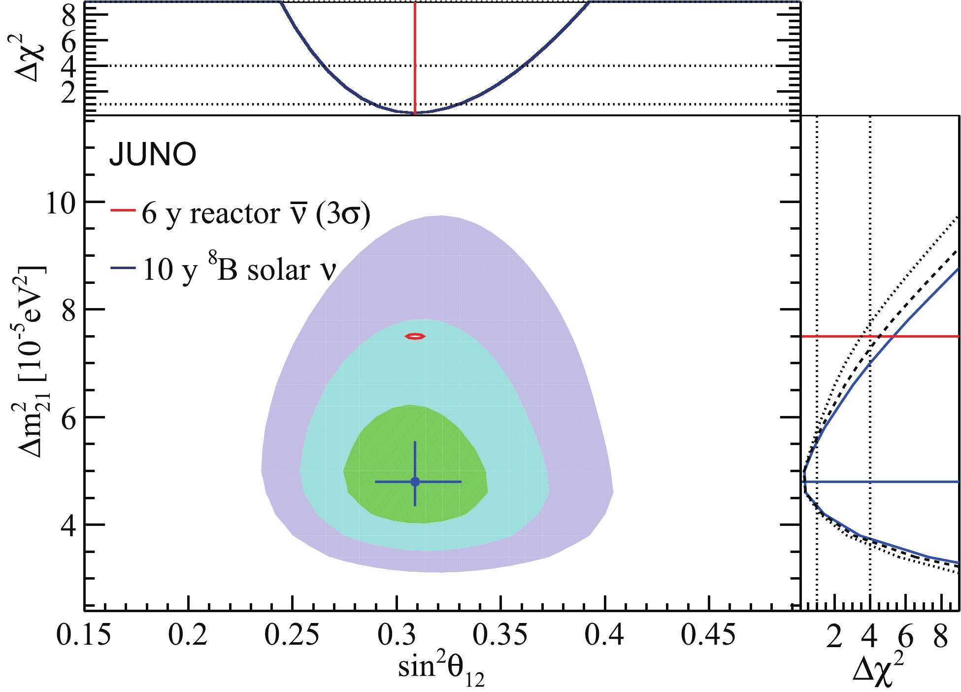
Figure 14. (color online) 68.3%, 95.5%, and 99.7% C.L. allowed regions in the
$\sin^2\theta_{12}$ and$\Delta m^2_{21}$ plane using the$^8$ B solar neutrino for ten years of data acquisition. The 99.7% C.L. region using six years of reactor$\overline{\nu}_{e}$ data is drawn in red for comparison, in which the$\Delta m^2_{21}$ central value is set to KamLAND's result [20], and uncertainties are taken from the JUNO Yellow Book [22]. The one-dimensional$\Delta\chi^2$ values for$\sin^2\theta_{12}$ and$\Delta m^2_{21}$ are shown in the top and right panels, respectively. The dashed line in the right panel represents the$\Delta m^2_{21}$ precision without$^{208}$ Tl reduction, while the dotted line shows the results with an analysis threshold limited to 5 MeV because of intrinsic$^{238}$ U and$^{232}$ Th contaminations at the 10$^{-15}$ g/g level.A crucial input to this study is the LS intrinsic radioactivity level. The current result is based on the assumption of achieving
$ 10^{-17} $ g/g$ ^{238} $ U and$ ^{232} $ Th as well as a 2,600 cpd/kt$ ^{210} $ Po decay rate. If the$ ^{210} $ Po decay rate becomes greater than 10,000 cpd/kt, such as that in the Phase I of Borexino,$ ^{208} $ Tl cannot be reduced by the$ ^{212} $ Bi$ - $ $ ^{208} $ Tl cascade decay, and the S/B ratio decreases from 35 to 0.6 in the 3 to 5 MeV energy range. The effect on the$ \Delta m^2_{21} $ precision is shown as the dashed line in the right panel of Fig. 14. If the$ ^{238} $ U and$ ^{232} $ Th contaminations are at the$ 10^{-15} $ g/g level, the analysis threshold would be limited to 5 MeV. The$ \Delta m^2_{21} $ measurement would mostly rely on the Day-Night asymmetry, and the projected sensitivity is shown as the dotted line in the right panel of Fig. 14. In this case, the sensitivity of distinguishing the two$ \Delta m^2_{21} $ values is slightly worse than 2$ \sigma $ ($ \Delta\chi^2\sim 3.5 $ ). However, if$ ^{238} $ U and$ ^{232} $ Th contaminations are smaller than 10$ ^{-17} $ g/g, the sensitivities do not have significant improvements, as the background in the 2 to 5 MeV energy range is dominated by cosmogenic$ ^{10} $ C and$ ^{6} $ He in this case. -
More than fifty years after the discovery of solar neutrinos, they continue to provide the potential for major contributions to neutrino physics. The JUNO experiment, with a 20 kt LS detector, can shed light on the current inconsistency between
$ \Delta m^2_{21} $ values measured using solar neutrinos and reactor antineutrinos. Compared with the discussion in the JUNO Yellow Book [22], a set of energy-dependent FV cuts is newly designed based on comprehensive background studies, leading to a maximized target mass with negligible external background. The veto strategies for cosmogenic isotopes are also improved compared with those in Refs. [22, 63]. A set of distance-dependent veto time cuts is developed for the cylindrical veto along the muon track, resulting in a significantly improved signal to background ratio. With 10$ ^{-17} $ g/g intrinsic$ ^{238} $ U and$ ^{232} $ Th, the analysis threshold of recoil electrons from the ES channel can be reduced from the current value of 3 MeV at Borexino [23] to 2 MeV. In the standard three-flavor neutrino oscillation framework, the spectrum distortion and the Day-Night asymmetry lead to a$ \Delta m^2_{21} $ measurement of$ 4.8^{+0.8}_{-0.5}\; (7.5^{+1.6}_{-1.2})\times 10^{-5} $ eV$ ^2 $ , with a precision similar to that of the current solar global fitting result.The interactions between neutrinos and carbon, such as
$ \nu_x $ -$ ^{12} $ C NC and$ \nu_{e} $ -$ ^{13} $ C CC channels, are under investigation. Most of the neutrino energy is carried by electrons in the CC reactions, and it can also be used for examination of the spectrum distortion. Furthermore, both channels could be utilized in the search for$ hep $ solar neutrinos, which have a predicted arrival flux of$ 8.25\times10^3 $ /cm$ ^2 $ /s but have not been detected yet. -
We are grateful for the ongoing cooperation from the China General Nuclear Power Group.
Feasibility and physics potential of detecting 8B solar neutrinos at JUNO
- Received Date: 2020-06-26
- Available Online: 2021-02-15
Abstract: The Jiangmen Underground Neutrino Observatory (JUNO) features a 20 kt multi-purpose underground liquid scintillator sphere as its main detector. Some of JUNO's features make it an excellent location for


 DownLoad: