


 Abstract
 HTML
HTML Reference
 Related
 PDF
PDF


-
The widely used nonrelativistic QCD (NRQCD) factorization [1] has encountered notable difficulties in describing heavy quarkonium data. As the NRQCD factorization is based on the NRQCD effective field theory [2], it is likely rigorous, although for inclusive quarkonium production, only two-loop verification is available at present [3-5]. The main known problem of NRQCD factorization is the bad convergence of its relativistic expansion [6], which may be responsible for its deficiencies. Recently, a new factorization approach called soft gluon factorization (SGF) [7,8] was proposed to describe quarkonium production and decay. The aim of SGF is to resum the series of relativistic corrections originating from the kinematic effects in NRQCD, which are the main cause of the poor convergence of the relativistic expansion.
Nevertheless, SGF has not been well-established. In SGF, the hadronization of intermediate quark-antiquark pairs to physical quarkonium is described by nonperturbative soft gluon distributions (SGDs), which are only formally defined by QCD fields in a small loop momentum region [7]. Without an explicit definition of a small region, it is hard to prove the validity of SGF for physical processes. Furthermore, the unclear relation between SGF and NRQCD factorization makes it impossible to verify whether the kinematic effects have been correctly resummed.
In this paper, with the help of a new regulator, we provide a rigorous definition of a small region in SGF. We then present two strategies for exploring the relationship between SGF and NRQCD factorization. In the first strategy, we apply the two factorization theories to the physical process of
$ J/\psi \to e^+e^- $ and show that both SGF and NRQCD factorization can correctly reproduce all the low energy physics of full QCD in this process. In the second strategy, we argue that the SGF formula can be deduced from NRQCD at the operator level by using equations of motion. Both strategies demonstrate that SGF and NRQCD factorization are equivalent, which means that, for any process, the two factorizations theories are either both valid or both violated. By identifying the two theories, we generate complete relations between the nonperturbative matrix elements in SGF and NRQCD; this proves the generalized Gremm-Kapustin relation [9] as a byproduct.The rest of this paper is organized as follows. In Sec. II, we study the exclusive process
$ J/\psi \to e^+e^- $ in SGF. We give a rigorous definition of nonperturbative matrix elements in SGF and show that the low energy physics of full QCD can be reproduced by SGF. In Sec. III, we discuss the equivalence between SGF and NRQCD factorization and establish relations between the nonperturbative matrix elements in SGF and NRQCD. In Sec. IV, we show that SGF can be deduced from NRQCD at the operator level. We summarize our results in Sec. V. Some of the technical details of our calculations are provided in Appendix A. -
According to Ref. [8], for the exclusive decay process, we have the following SGF formula at the amplitude level:
$ {\cal{A}}^{ {\cal Q}} = \sum\limits_{n} \hat{{\cal{A}} }^{n} \overline{R}^{n*}_{ {\cal Q}}, $

(1) where
$ n $ denotes intermediate states. In general,$ n $ can contain dynamical soft partons (gluons or light quarks) in addition to a$ Q\bar Q $ pair. However, for simplicity, in this work we only discuss intermediate states without dynamical soft partons, which can nevertheless be treated similarly. The nonperturbative matrix elements$ \overline{R}^{n*}_{{ {\cal Q}}} $ are then defined as$ \overline{R}^{n*}_{ {\cal Q}} = \langle 0|[\overline\Psi {\cal{K}}_{n}\Psi](0) |{ {\cal Q}}\rangle_S, $

(2) where
$ \Psi $ stands for the Dirac field of a heavy quark,$ {\cal{K}}_{n} $ is the projection operator defining the intermediate state$ n $ , and the subscript "S" indicates that, to evaluate the matrix elements, one only includes integration regions where the off-shellness of all particles is much smaller than the heavy-quark mass. From the point view of the method of regions [10,11], the effect of "S" is to keep only small regions, which include everything except the hard regions.For the process
$ J/\psi \to e^+e^- $ , the symmetries of QCD tell us that only$ n = {^{{3}}{S}_{{1}}^{[{1}]}}, {^{{3}}{D}_{{1}}^{[{1}]}} $ are relevant, where the spectroscopic notation, with the superscript "[1]", denotes a color singlet. We thus have$ {\cal{A}}^{J/\psi \to e^+e^- } = \hat{{\cal{A}}}^{ {^{{3}}{S}_{{1}}^{[{1}]}}}\overline{R}^{ {^{{3}}{S}_{{1}}^{[{1}]}} *}_{J/\psi} + \hat{{\cal{A}}}^{ {^{{3}}{D}_{{1}}^{[{1}]}}}\overline{R}^{ {^{{3}}{D}_{{1}}^{[{1}]}} *}_{J/\psi}, $

(3) with the projection operators defined explicitly as
$\tag{4a} {\cal{K}}_{ {^{{3}}{S}_{{1}}^{[{1}]}}} = \frac{\sqrt{M}}{M+2m}\frac{M-{\not\!\! P}}{2M}{\epsilon}_{S_z}^{*\mu} \gamma_\mu\frac{M+{\not\!\! P}}{2M}{\cal C}^{[1]}, $

$\tag{4b} \begin{aligned}[b] {\cal{K}}_{ {^{{3}}{D}_{{1}}^{[{1}]}}} = & \frac{\sqrt{M}}{M+2m}\frac{M-{\not\!\! P}}{2M} {\epsilon}_{S_z}^{*\mu}\gamma^\nu \frac{M+{\not\!\! P}}{2M}{\cal C}^{[1]}(-\frac{\rm i}{2})^2 \overleftrightarrow{D}^\alpha \overleftrightarrow{D}^\beta\\ &\times ( \mathbb{P}_{\alpha\mu}\mathbb{P}_{\beta\nu} -\frac{1}{d-1} \mathbb{P}_{\alpha\beta} \mathbb{P}_{\mu\nu} ) { \sqrt{\frac{2(d-1)}{(d-2)(d+1)}}}, \end{aligned} $

where
$ d = 4-2\epsilon $ is the space-time dimension,$ D_\mu $ is the gauge covariant derivative with$ \overline\Psi \overleftrightarrow{D}_\mu \Psi = \overline\Psi (D_\mu \Psi) - $ $(D_\mu \overline\Psi)\Psi $ ,$ P $ is the momentum of$ J/\psi $ ,$ {\epsilon}_{S_z}^{\mu} $ is a polarization vector with$ P\cdot {\epsilon}_{S_z} = 0 $ ,$ m $ is the heavy-quark mass,$ M $ is the mass of$ J/\psi $ , the color projector is defined as$ {\cal C}^{[1]} = 1/\sqrt{N_c} $ , and the spin projection operator$ \mathbb{P}_{\alpha\beta} $ is defined as$ \mathbb{P}_{\alpha\beta} = -g_{\alpha\beta}+\frac{P_\alpha P_\beta}{P^2}. $

(5) The hard parts
$ \hat{{\cal{A}}}^{n} $ can be perturbatively calculated according to the matching procedure discussed in [7,8]. To this end, we first replace$ J/\psi $ with an on-shell color-singlet state$ c\bar{c}( {^{{3}}{S}_{{1}}^{[{1}]}}) $ with momenta①$ p_c = P/2+q, \quad p_{\overline{c}} = P/2-q $

(6) on both sides of Eq. (3). The on-shell conditions
$ p_c^2 = p_{\overline{c}}^2 = m^2 $ result in$ P\cdot q = 0, \quad \quad q^2 = m^2-M^2/4, $

(7) which fixes
$ q_0 $ and$ |{{q}}| $ in the rest frame of$ P $ . The remaining degrees of freedom of$ q $ are removed by partial wave expansion, i.e.,$ S $ -wave expansion in this case. After the replacement, the l.h.s. of Eq. (3) becomes$ {\cal{A}}^{c\bar{c}( {^{{3}}{S}_{{1}}^{[{1}]}})\to e^+e^-} = (-{\rm i} ee_q)\frac{-{\rm i}}{M^2}L_{\mu } \int \frac{{\rm d}^2\Omega}{4\pi} {{\rm{Tr}}}\left[ \Pi_{1S_z} {\cal{A}}^{\mu }_{c\bar c}\right], $

(8) where
$ \Omega $ is the solid angle of the relative momentum$ {{q}} $ in the$ c\bar{c} $ rest frame,$ L_\mu $ is the leptonic current with$ L_{\mu } = -{\rm i} e\,\overline{u}(k_{e^-})\gamma_{\mu} v(k_{e^+}), $

(9) and
$ {\cal{A}}^{\mu }_{c\bar c} $ is the hadronic part of the decay amplitude with the spinors of$ c\bar{c} $ removed. The$ c\bar{c} $ pair is projected to state$ {^{{3}}{S}_{{1}}^{[{1}]}} $ by replacing the spinors of the$ c\bar{c} $ pair by$ {\Pi}_{1S_z} = \frac{({\not\!\! p}_{{c}}+m) \dfrac{M+{\not \!\!P}}{2M} {\epsilon}_{S_z}^{\mu} \gamma_\mu \dfrac{M-{\not \!\!P}}{2M} ({\not\!\! p}_{\overline{c}}-m)}{\sqrt{M}(M/2+m)}{\cal C}^{[1]}. $

(10) Similarly, we have
$\tag{11a} \overline{R}^{ {^{{3}}{S}_{{1}}^{[{1}]}} *}_{c\bar{c}( {^{{3}}{S}_{{1}}^{[{1}]}})} = \int \frac{{\rm d}^2\Omega}{4\pi} {{\rm{Tr}}}[ \Pi_{1S_z} \overline{R}^{ {^{{3}}{S}_{{1}}^{[{1}]}} *}_{c \bar{c}}], $

$\tag{11b} \overline{R}^{ {^{{3}}{D}_{{1}}^{[{1}]}} *}_{c\bar{c}( {^{{3}}{S}_{{1}}^{[{1}]}})} = \int \frac{{\rm d}^2\Omega}{4\pi} {{\rm{Tr}}}[ \Pi_{1S_z} \overline{R}^{ {^{{3}}{D}_{{1}}^{[{1}]}} *}_{c \bar{c}}]. $

Based on these equations, one can calculate
$ {\cal{A}}^{c\bar{c}( {^{{3}}{S}_{{1}}^{[{1}]}})\to e^+e^-} $ ,$ \overline{R}^{ {^{{3}}{S}_{{1}}^{[{1}]}} *}_{c\bar{c}( {^{{3}}{S}_{{1}}^{[{1}]}})} $ , and$ \overline{R}^{ {^{{3}}{D}_{{1}}^{[{1}]}} *}_{c\bar{c}( {^{{3}}{S}_{{1}}^{[{1}]}})} $ perturbatively.Denoting the perturbative expansion of any quantity
$ W $ as$ W = W^{(0)}+\alpha_s W^{(1)}+\alpha_s^2 W^{(2)}+\cdots $ , we have the following orthogonal relations [7]:$\tag{12a} \overline{R}^{ {^{{3}}{S}_{{1}}^{[{1}]}} *,(0)}_{c\bar{c}( {^{{3}}{S}_{{1}}^{[{1}]}})} = 1, $

$\tag{12b} \overline{R}^{ {^{{3}}{D}_{{1}}^{[{1}]}} *,(0)}_{c\bar{c}( {^{{3}}{S}_{{1}}^{[{1}]}})} = 0. $

Based on this, Eq. (3) results in the following matching relations:
$\tag{13a} \hat{{\cal{A}}}^{ {^{{3}}{S}_{{1}}^{[{1}]}},(0)} = {\cal{A}}^{c\bar{c}( {^{{3}}{S}_{{1}}^{[{1}]}}) \to e^+e^-,(0) }, $

$\tag{13b}\begin{aligned}[b] \hat{{\cal{A}}}^{ {^{{3}}{S}_{{1}}^{[{1}]}},(1)} = &{\cal{A}}^{c\bar{c}( {^{{3}}{S}_{{1}}^{[{1}]}}) \to e^+e^-,(1) }-\hat{{\cal{A}}}^{ {^{{3}}{S}_{{1}}^{[{1}]}},(0)}\overline{R}^{ {^{{3}}{S}_{{1}}^{[{1}]}} *,(1)}_{c\bar{c}( {^{{3}}{S}_{{1}}^{[{1}]}})}\\&-\hat{{\cal{A}}}^{ {^{{3}}{D}_{{1}}^{[{1}]}},(0)}\overline{R}^{ {^{{3}}{D}_{{1}}^{[{1}]}} *,(1)}_{c\bar{c}( {^{{3}}{S}_{{1}}^{[{1}]}})},\\&\vdots\end{aligned} $

By replacing
$ J/\psi $ with$ c\bar{c}( {^{{3}}{D}_{{1}}^{[{1}]}}) $ , we can obtain similar relations for$ \hat{{\cal{A}}}^{ {^{{3}}{D}_{{1}}^{[{1}]}}} $ . These relations enable us to calculate$ \hat{{\cal{A}}}^{ {^{{3}}{S}_{{1}}^{[{1}]}}} $ and$ \hat{{\cal{A}}}^{ {^{{3}}{D}_{{1}}^{[{1}]}}} $ perturbatively. For simplicity, we concentrate on the S-wave contribution$ \hat{{\cal{A}}}^{ {^{{3}}{S}_{{1}}^{[{1}]}}} $ in the rest of the paper. -
We first calculate
$ {\cal{A}}^{c\bar{c}( {^{{3}}{S}_{{1}}^{[{1}]}}) \to e^+e^-} $ according to Eq. (8). The amplitude$ {\cal{A}}^\mu_{c\bar c} $ in full QCD can be decomposed as$ {\cal{A}}^\mu_{c\bar c} = {\cal{G}}\gamma^\mu + {\cal{H}}q^\mu , $

(14) and up to order
$ \alpha_s $ , one has [9]$\tag{15a} \begin{aligned}[b] {\cal{G}} =& 1+ \frac{\alpha_s C_F}{4\pi} [ 2[ (1+\delta^2)L(\delta) -1 ] (\frac{1}{\epsilon_{IR}} + \log \frac{4\pi \mu^2 e^{-\gamma_E}}{ m^2 } ) \\&+ 6\delta^2L(\delta) -4(1+\delta^2)K(\delta) - 4 + (1+\delta^2)\frac{\pi^2}{\delta}] +{\cal{O}}(\alpha_s^2), \end{aligned} $

$\tag{15b} {\cal{H}} = \frac{\alpha_s C_F}{4\pi} \frac{2(1-\delta^2)L(\delta)}{m} +{\cal{O}}(\alpha_s^2) , $

with
$ \begin{aligned}[b] \delta = & \frac{\sqrt{M^2-4m^2}}{M},\\ L(\delta) =& \frac{1}{2\delta} \log ( \frac{1+\delta}{1-\delta} ),\\ K(\delta) = & \frac{1}{4\delta} [ {{\rm{Li}}}_2(\frac{2\delta}{1+\delta} )- {{\rm{Li}}}_2(-\frac{2\delta}{1-\delta} ) ], \end{aligned} $

(16) where
$ {\rm{Li}}_2 $ is the Spence function:$ {\rm{Li}}_2(x) = \int_x^0 {\rm d} t \frac{\log(1-t)}{t}. $

(17) In the above results, we have dropped imaginary parts that are irrelevant for our purpose. By inserting Eqs. (14) and (10) into Eq. (8), one gets
$\begin{aligned}[b] {\cal{A}}^{c\bar{c}( {^{{3}}{S}_{{1}}^{[{1}]}})\to e^+e^-} =& \frac{ee_q}{M^2} \frac{(2(d-2)M + 4m){\cal{G}}- (M^2- 4m^2){\cal{H}}}{(d-1)\sqrt{M}} \\&\times\sqrt{N_c} {L} \cdot {\epsilon}_{S_z}. \end{aligned} $

(18) Note that in Ref. [9],
$ M $ is a free parameter, but to use these expressions for SGF, it needs to be the quarkonium mass. -
We now describe our method for calculating
$ \overline{R}^{ {^{{3}}{S}_{{1}}^{[{1}]}} *}_{c\bar{c}( {^{{3}}{S}_{{1}}^{[{1}]}})} $ . As pointed out in Refs. [7,8], this quantity has been defined to include only small loop momentum regions. In what follows, we provide an explicit definition and choose a UV renormalization scheme.Up to order
$ \alpha_s $ , the corresponding Feynman diagrams are shown in Fig. 1, where the solid circle represents the operator$ \overline\Psi {\cal{K}}_{ {^{{3}}{S}_{{1}}^{[{1}]}}}\Psi $ . The calculation at the tree level is straightforward; the result is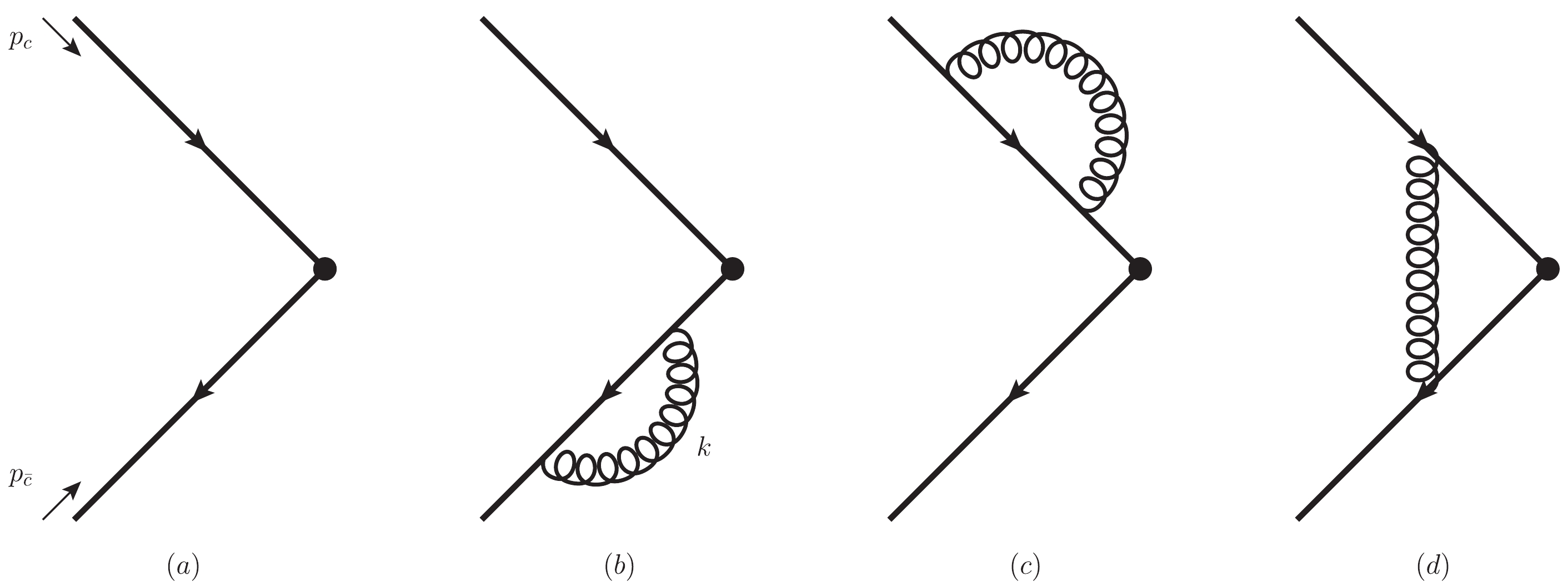
Figure 1. Feynman diagrams for the
$ {^{{3}}{S}_{{1}}^{[{1}]}} $ matrix element$ \overline{R}^{c\bar{c}( {^{{3}}{S}_{{1}}^{[{1}]}})*,(0)}_{c\bar{c}( {^{{3}}{S}_{{1}}^{[{1}]}})} = \int \frac{{\rm d}^2\Omega}{4\pi} {\rm{Tr}} [ {\cal{K}}_{ {^{{3}}{S}_{{1}}^{[{1}]}}} \Pi_{1S_z} ] = 1. $

(19) Consider the vertex correction in Fig. 1(d) as an example to explain the calculation at the one-loop level. The amplitude reads
$ \overline{R}^{c\bar{c}( {^{{3}}{S}_{{1}}^{[{1}]}})*}_{c\bar{c}( {^{{3}}{S}_{{1}}^{[{1}]}})}\vert_{d} = (-{\rm i} g_s^2\mu^{2\epsilon})\int \frac{{\rm d}^2\Omega}{4\pi}\int \frac{{\rm d}^dk}{(2\pi)^d} T_S\left\{ \frac{ {\rm{Tr}} [\gamma^\alpha (-{\not\!\! p}_{{\bar c }}+{\not\!\! k}+m)T^a {\cal{K}}_{ {^{{3}}{S}_{{1}}^{[{1}]}}} T^a ({\not\!\! p}_{{ c }}+ {\not\!\! k} +m) \gamma_\alpha \Pi_{1S_z} ]}{[k^2+{\rm i}0^+][k^2-2p_{\bar c}\cdot k +{\rm i}0^+][k^2+2p_{ c}\cdot k +{\rm i}0^+]}\right\}, $

(20) where
$ T_S $ is an operator that forces the loop momentum$ k $ to be in a small region [7,8], which will be defined explicitly by using the method of regions [10,11].Before continuing, we note that, although the full QCD integral in Eq. (20) is well regularized by dimensional regularization, the manipulation to define
$ T_S $ generates unregularized integrals. Therefore, another regulator is needed to make our manipulation mathematically rigorous. We thus propose a new regularization at the full QCD level by multiplying the power of all propagator denominators by$ 1+\eta $ ; this can regularize all possible divergences encountered in the derivation using the method of regions, including both ultraviolet and non-ultraviolet divergences②. A similar regularization method has been used in the light-cone ordered perturbation theory in Ref. [12] to regularize rapidity divergences. For the integral of interest, we obtain$ \overline{R}^{c\bar{c}( {^{{3}}{S}_{{1}}^{[{1}]}})*}_{c\bar{c}( {^{{3}}{S}_{{1}}^{[{1}]}})}\vert_{d} = (-{\rm i}g_s^2\mu^{2\epsilon})\int \frac{{\rm d}^2\Omega}{4\pi}\int \frac{{\rm d}^dk}{(2\pi)^d} T_S\left\{ \frac{\nu^{3\eta} {\rm{Tr}} [\gamma^\alpha (-{\not\!\! p}_{{\bar c }}+{\not \!\! k}+m)T^a {\cal{K}}_{ {^{{3}}{S}_{{1}}^{[{1}]}}} T^a ({\not\!\! p}_{{ c }}+ {\not\!\! k} +m) \gamma_\alpha \Pi_{1S_z} ]}{[k^2+{\rm i}0^+]^{1+\eta}[k^2-2p_{\bar c}\cdot k +{\rm i}0^+]^{1+\eta}[k^2+2p_{ c}\cdot k +{\rm i}0^+]^{1+\eta}}\right\}+O(\eta), $

(21) where
$ \nu $ is introduced to compensate for the change in mass dimension caused by the new regularization, and we assume$ \eta\ll \epsilon $ to ensure that the theory can eventually be regularized by dimensional regularization.With the new regularization at hand, we decompose the loop momentum
$ k_\mu = (k_0,{{k}}) $ into three domains:$ \begin{array}{l} { {\rm{the\; hard\; domain}}: D_h = \{k\in D: {|k_{0}|} \gg |{{q}}| \vee |{{k}}| \gg |{{q}}| \}},\\ { {\rm{the\; soft\; domain}}: D_s = \{k\in D: |{{k}}| \lesssim {|k_{0}|} \lesssim |{{q}}| \}}, \\ { {\rm{the\; potential\; domain}}: D_p = \{k\in D: {|k_{0}|} \ll |{{k}}| \lesssim |{{q}}| \}}, \end{array} $

(22) where the relation "
$ \lesssim $ " is understood as the negation of "$ \gg $ ,"$ D = \mathbb{R}^{d} $ is the complete integration domain, and an implicit cutoff scale exists to rigorously separate the three domains. This division satisfies$ \begin{aligned}[b] &D_i \cap D_j = \emptyset, \quad i,j \in \{h,s,p \}\; {\rm{and}}\; i\neq j, \\ D_h & \cup D_s \cup D_p = D. \end{aligned} $

(23) Then, one can split any original integral
$ F $ into the three domains:$ F \equiv \int {\rm d}^dk I(k,P,q) = \int_{k\in D_h} {\rm d}^dk I + \int_{k\in D_s} {\rm d}^dk I +\int_{k\in D_p} {\rm d}^dk I. $

(24) A possible definition of
$ T_S $ is$ \{k\in D_s\cup D_p\} $ . However, this definition involves a hard cutoff, which makes high order perturbative calculations inconvenient.To obtain a more convenient definition, we introduce the operators
$ T^{(i)}\; (i \in \{h,s,p \}) $ , which expand the integrand to a convergent power series of small quantities in each domain. We also define
$ T^{(i,j,\cdots)}\equiv T^{(i)}T^{(j,\cdots)} $ . We then have$ \begin{aligned}[b] \int_{k\in D_s} {\rm d}^dk I +\int_{k\in D_p} {\rm d}^dk I = &\int_{k\in D_s} {\rm d}^dk T^{(s)}I +\int_{k\in D_p} {\rm d}^dk T^{(p)}I\\ = & \int {\rm d}^dk T^{(s)}I-\int_{k\in D_h} {\rm d}^dk T^{(s)}I-\int_{k\in D_p} {\rm d}^dk T^{(s)}I +\int {\rm d}^dk T^{(p)}I-\int_{k\in D_h} {\rm d}^dk T^{(p)}I-\int_{k\in D_s} {\rm d}^dk T^{(p)}I\\ = & \int {\rm d}^dk T^{(s)}I-\int_{k\in D_h} {\rm d}^dk T^{(h,s)}I-\int_{k\in D_p} {\rm d}^dk T^{(p,s)}I +\int {\rm d}^dk T^{(p)}I-\int_{k\in D_h} {\rm d}^dk T^{(h,p)}I-\int_{k\in D_s} {\rm d}^dk T^{(s,p)}I\\ = & \int {\rm d}^dk \bigg\{T^{(s)}+ T^{(p)}- T^{(s,p)}\bigg\}I-\int_{k\in D_h} {\rm d}^dk \bigg\{ T^{(h,s)} + T^{(h,p)}- T^{(h,s,p)}\bigg\}I, \end{aligned} $

(25) where the property
$ T^{(i,j)} = T^{(j,i)} $ has been used [11]. It is clear that the l.h.s. and the first term on the r.h.s. of this equation are equivalent in the low energy domain and that their difference is an integration in the hard domain, which is infrared safe but may be ultraviolet divergent. The difference can be interpreted as a different choice of renormalization scheme. Therefore, we arrive at our final definition:$ T_S = T^{(s)}+ T^{(p)}- T^{(s,p)}, $

(26) with the UV divergences removed by an
$ \overline{ {{\rm{MS}}}} $ renormalization scheme.$ T^{(s)} $ and$ T^{(p)} $ are conventionally respectively called the soft region and potential region, while the overlap region$ T^{(s,p)} $ compensates for the double counting between$ T^{(s)} $ and$ T^{(p)} $ .For the soft region contribution
$ \overline{R}^{c\bar{c}( {^{{3}}{S}_{{1}}^{[{1}]}})*,{(s)}}_{c\bar{c}( {^{{3}}{S}_{{1}}^{[{1}]}})} $ , we apply the operator$ T^{(s)} $ to expand the integrand in Eq. (21) for small quantities. This results in the following integrals:$ \int \frac{{\rm d}k_0 {\rm d}^{d-1}{{k}}}{(2\pi)^d} \frac{k_0^{m_1} ( {{k}}\cdot {{q}})^{m_2}(-k_0^2)^{j_{14}}({{k}}^{2})^{j_{25}}(2 {{k}}\cdot {{q}})^{j_{36}} }{[k_0^2 - {{k}}^{2} + {\rm i}0^+]^{1+\eta}[ P_0k_0 +{\rm i}0^+]^{1+\eta+j_{123}}[ - P_0k_0 +{\rm i}0^+]^{1+\eta+j_{456}}}, $

(27) where the term
$ k_0^{m_1} ( {{k}}\cdot {{q}})^{m_2} $ comes from the numerator in Eq. (21), and$ j_{\alpha\beta\cdots} \equiv j_{\alpha} + j_{\beta} +\cdots, $

(28) where
$ j_i $ are non-negative integers. As scaleless and infrared-finite integrals can be set to zero (which is another choice of scheme), we find that only integrals with$ m_1 = m_2 = j_1 = j_2 = j_4 = j_5 = 0 $ are relevant:$ \int \frac{{\rm d}k_0 {\rm d}^{d-1}{{k}}}{(2\pi)^d} \frac{(2 {{k}}\cdot {{q}})^{j_{36}} }{[k_0^2 - {{k}}^{2} + {\rm i}0^+]^{1+\eta}[ P_0k_0 +{\rm i}0^+]^{1+\eta+j_{3}}[ - P_0k_0 +{\rm i}0^+]^{1+\eta+j_{6}}}. $

(29) These integrals have pinch poles around
$ k_0 = 0 $ that can be regularized by the new regulator$ \eta $ . As integrals in$ \overline{R}^{c\bar{c}( {^{{3}}{S}_{{1}}^{[{1}]}})*,{(s,p)}}_{c\bar{c}( {^{{3}}{S}_{{1}}^{[{1}]}})} $ can be obtained by expanding the$ k_0^2 $ term in the denominator in Eq. (29), it is clear that they cancel exactly with the contribution of the pinch poles around$ k_0 = 0 $ in$ \overline{R}^{c\bar{c}( {^{{3}}{S}_{{1}}^{[{1}]}})*,{(s)}}_{c\bar{c}( {^{{3}}{S}_{{1}}^{[{1}]}})} $ . This cancellation demonstrates that the overlap region is conceptually important even though it contains only scaleless integrals that are usually set to zero in dimensional regularization. In fact, such overlap contributions have also been introduced as "zero-bin subtraction" in effective-theory treatments [13,14]; this resolves a number of problems in effective theories (NRQCD and soft-collinear effective theory) [13], including the pinch singularity problem discussed above. By combining the soft region and the overlap region, we only need to consider the contribution from the gluon pole, and we can safely take the limit$ \eta\to 0 $ , which results in$ \overline{R}^{ {^{{3}}{S}_{{1}}^{[{1}]}}*,(s)}_{c\bar{c}( {^{{3}}{S}_{{1}}^{[{1}]}})} -\overline{R}^{ {^{{3}}{S}_{{1}}^{[{1}]}}*,(s,p)}_{c\bar{c}( {^{{3}}{S}_{{1}}^{[{1}]}})} \vert_{d} = \frac{\alpha_sC_F}{4\pi} 2(1+\delta^2)L(\delta) (\frac{1}{\epsilon_{IR}} -\frac{1}{\epsilon_{UV}} ) . $

(30) We emphasize that, if one wants to calculate
$ \overline{R}^{ {^{{3}}{S}_{{1}}^{[{1}]}}*,(s)}_{c\bar{c}( {^{{3}}{S}_{{1}}^{[{1}]}})} $ separately, the correct order is to first integrate over$ k_0 $ with fixed$ {{k}} $ . Otherwise, the poles around$ k_0 = 0 $ will be regularized by different regulators between the soft region and overlap region, which necessarily breaks the symmetries of the theory and makes the cancellation between the two regions impossible.For
$ \overline{R}^{c\bar{c}( {^{{3}}{S}_{{1}}^{[{1}]}})*,{(p)}}_{c\bar{c}( {^{{3}}{S}_{{1}}^{[{1}]}})} $ , the terms in the expansion are proportional to$ \int \frac{{\rm d}k_0 {\rm d}^{d-1}{{k}}}{(2\pi)^d} \frac{k_0^{m_1} ( {{k}}\cdot {{q}})^{m_2}(-k_0^2)^{j_{123}} }{[- {{k}}^{2} + {\rm i}0^+]^{1+\eta+j_3}[- {{k}}^{2}+ P_0k_0 - 2 {{k}}\cdot {{q}} +{\rm i}0^+]^{1+\eta+j_{1}}[ - {{k}}^{2} - P_0k_0 - 2 {{k}}\cdot {{q}} +{\rm i}0^+]^{1+\eta+j_{2}}}, $

(31) where we can take
$ \eta\to 0 $ as all divergences are well regularized by dimensional regularization. Then because$ k_0 $ and$ {{k}}\cdot {{q}} $ can be expressed as linear combinations of the denominators, if any of$ m_1, m_2, j_1, j_2 $ , or$ j_3 $ is nonzero, the integral can be decomposed to either scaleless and infrared-finite integrals or to integrals with pure virtual value. By keeping only the real part, we get$ \overline{R}^{ {^{{3}}{S}_{{1}}^{[{1}]}}*,(p)}_{c\bar{c}( {^{{3}}{S}_{{1}}^{[{1}]}})} \vert_{d} = \frac{\alpha_s C_F}{4\pi} (1+\delta^2 )\frac{\pi^2}{\delta} . $

(32) Similarly, for the self-energy diagrams, one can derive
$ \begin{aligned}[b] \overline{R}^{ {^{{3}}{S}_{{1}}^{[{1}]}}*,(s)}_{c\bar{c}( {^{{3}}{S}_{{1}}^{[{1}]}})} -\overline{R}^{ {^{{3}}{S}_{{1}}^{[{1}]}}*,(s,p)}_{c\bar{c}( {^{{3}}{S}_{{1}}^{[{1}]}})} \vert_{b+c} = & \frac{\alpha_sC_F}{2\pi} ( \frac{1}{\epsilon_{UV}} -\frac{1}{\epsilon_{IR}} ) ,\\ \overline{R}^{ {^{{3}}{S}_{{1}}^{[{1}]}}*,(p)}_{c\bar{c}( {^{{3}}{S}_{{1}}^{[{1}]}})} \vert_{b+c} = & 0. \end{aligned} $

(33) Summing these contributions, we obtain the matrix element at NLO before renormalization:
$ \begin{aligned}[b] \overline{R}^{ {^{{3}}{S}_{{1}}^{[{1}]}}*,(1)}_{c\bar{c}( {^{{3}}{S}_{{1}}^{[{1}]}})} \vert_{ {\rm{bare}}} = &\overline{R}^{ {^{{3}}{S}_{{1}}^{[{1}]}}*,(s)}_{c\bar{c}( {^{{3}}{S}_{{1}}^{[{1}]}})} -\overline{R}^{ {^{{3}}{S}_{{1}}^{[{1}]}}*,(s,p)}_{c\bar{c}( {^{{3}}{S}_{{1}}^{[{1}]}})} +\overline{R}^{ {^{{3}}{S}_{{1}}^{[{1}]}}*,(p)}_{c\bar{c}( {^{{3}}{S}_{{1}}^{[{1}]}})}\vert_{b+c+d}\\ = & \frac{\alpha_sC_F}{4\pi} [ (\frac{1}{\epsilon_{IR}} -\frac{1}{\epsilon_{UV}} ) ( 2(1+\delta^2)L(\delta) - 2 ) \\&+ (1+ \delta^2) \frac{\pi^2}{\delta} ] . \end{aligned} $

(34) Ultraviolet divergences in the above result can be removed by the
$ \overline{ {{\rm{MS}}}} $ renormalization procedure, yielding the renormalized matrix element$\begin{aligned}[b] \overline{R}^{ {^{{3}}{S}_{{1}}^{[{1}]}}*}_{c\bar{c}( {^{{3}}{S}_{{1}}^{[{1}]}})} =& 1+ \frac{\alpha_sC_F}{4\pi} [ (\frac{1}{\epsilon_{IR}} + \ln(4\pi e^{-\gamma_E}) ) [ 2(1+\delta^2)L(\delta) - 2 ] \\&+ (1+ \delta^2) \frac{\pi^2}{\delta} ] +{\cal{O}}(\alpha_s^2). \end{aligned}$

(35) Similarly, because we find that the real part of
$ \overline{R}^{ {^{{3}}{D}_{{1}}^{[{1}]}} *,(1)}_{c\bar{c}( {^{{3}}{S}_{{1}}^{[{1}]}})} $ is proportional to$ \overline{R}^{ {^{{3}}{D}_{{1}}^{[{1}]}} *,(0)}_{c\bar{c}( {^{{3}}{S}_{{1}}^{[{1}]}})} $ , we have$ \overline{R}^{ {^{{3}}{D}_{{1}}^{[{1}]}} *,(1)}_{c\bar{c}( {^{{3}}{S}_{{1}}^{[{1}]}})} = 0. $

(36) -
Substituting Eqs. (18), (35), and (36) into Eq. (13), we obtain
$\tag{37a} \hat{{\cal{A}}}^{ {^{{3}}{S}_{{1}}^{[{1}]}},(0)} = \frac{ee_q}{M^2} \frac{4 (M + m)}{3\sqrt{M}} \sqrt{N_c} L \cdot {\epsilon}_{S_z} , $

$\tag{37b} \hat{{\cal{A}}}^{ {^{{3}}{S}_{{1}}^{[{1}]}},(1)} = \frac{ee_q}{M^2} \frac{4 (M + m){\cal{G}}^\prime- (M^2- 4m^2){\cal{H}}^\prime}{3\sqrt{M}} \sqrt{N_c}{L} \cdot {\epsilon}_{S_z}, $

where
$\tag{38a}\begin{aligned}[b] {\cal{G}}^\prime = &\frac{\alpha_s C_F}{4\pi} [ 2( (1+\delta^2)L(\delta) -1 ) \log ( \frac{\mu^2 }{ m^2 } ) \\&+ 6\delta^2 L(\delta) -4(1+\delta^2)K(\delta) - 4 ], \end{aligned} $

$\tag{38b} {\cal{H}}^\prime = \frac{\alpha_s C_F}{4\pi} \frac{2(1-\delta^2)L(\delta)}{m} . $

We find that the matrix element defined in SGF reproduces all infrared and Coulomb divergences in full QCD and that the obtained hard part is free of divergences. We therefore conclude that the SGF factorization holds at least at the one-loop level.
-
The correctness of SGF at the one-loop order can be understood in the following way. The full QCD results in Eq. (18) can also be reproduced by the method of regions (see Appendix A for details), in which
$ {\cal{A}}^{c\bar{c}( {^{{3}}{S}_{{1}}^{[{1}]}})\to e^+e^-} $ is expressed as$\begin{aligned}[b] {\cal{A}}^{c\bar{c}( {^{{3}}{S}_{{1}}^{[{1}]}})\to e^+e^-,(1)} =& \bigg\{{\cal{A}}^{(h)} -{\cal{A}}^{(h,s)}-{\cal{A}}^{(h,p)} +{\cal{A}}^{(h,s,p)} \bigg\} \\& + \bigg\{ {\cal{A}}^{(s)}+ {\cal{A}}^{(p)}-{\cal{A}}^{(s,p)} \bigg\}.\end{aligned} $

(39) Here, the first term on the r.h.s has nonzero support only in the hard domain and is thus infrared safe. It is straightforward to check that the low energy part of
$ {\cal{A}}^{c\bar{c}( {^{{3}}{S}_{{1}}^{[{1}]}})\to e^+e^-} $ has been correctly reproduced by the matrix element in SGF, i.e.,$ {\cal{A}}^{(s)}+ {\cal{A}}^{(p)}-{\cal{A}}^{(s,p)} = \hat{{\cal{A}}}^{ {^{{3}}{S}_{{1}}^{[{1}]}},(0)} \overline{R}^{ {^{{3}}{S}_{{1}}^{[{1}]}}*,(1)}_{c\bar{c}( {^{{3}}{S}_{{1}}^{[{1}]}})} \vert_{ {\rm{bare}}}, $

(40) which leaves the corresponding short-distance hard part defined by the high energy part of
$ {\cal{A}}^{c\bar{c}( {^{{3}}{S}_{{1}}^{[{1}]}})\to e^+e^-} $ , and thus, it is infrared safe. More precisely, we have$ \hat{{\cal{A}}}^{ {^{{3}}{S}_{{1}}^{[{1}]}},(1)} = \bigg\{{\cal{A}}^{(h)} -{\cal{A}}^{(h,s)}-{\cal{A}}^{(h,p)} +{\cal{A}}^{(h,s,p)} \bigg\}\bigg|_{\overline{ {\rm{MS}}}}, $

(41) where
$ \overline{ {\rm{MS}}} $ denotes the removal of UV divergences by the$ \overline{ {\rm{MS}}} $ subtraction scheme③.The above one-loop argument can be generalized to all orders. By definition, the low energy part (the "small" region of loop momenta) in full QCD can be reproduced by the matrix element in SGF at any order in the
$ \alpha_s $ expansion, with a proper definition of$ T_S $ at the multi-loop level as discussed in Ref. [11]. Therefore, the short-distance hard part is perturbatively infrared-safe, which means that the SGF formula for the decay width of$ J/\psi \to e^+e^- $ holds for all orders in$ \alpha_s $ . -
Ignoring operators involving gauge fields, the NRQCD factorization for the decay amplitude
$ J/\psi \to e^+e^- $ is given by [9,15,16]$\begin{aligned}[b] {\cal{A}}^{J/\psi \to e^+e^- } =& \sum\limits_{n} s_n( {^{{3}}{S}_{{1}}^{[{1}]}}) \langle 0 \vert {\cal{O}}_{An} \vert J/\psi \rangle \\&+ \sum\limits_{n} b_n( {^{{3}}{D}_{{1}}^{[{1}]}}) \langle 0 \vert {\cal{O}}_{Dn} \vert J/\psi \rangle, \end{aligned} $

(42) with④
$\tag{43a} \langle 0 \vert{\cal{O}}_{An} \vert J/\psi \rangle = \langle 0 | \chi^\dagger (-\frac{\rm i}{2} \overleftrightarrow{{\nabla}} )^{2n} {{\sigma}} \cdot {{\epsilon}}_{S_z}^{*} \psi | J/\psi \rangle , $

$\tag{43b}\begin{aligned}[b] \langle 0 \vert{\cal{O}}_{Dn} \vert J/\psi \rangle =& \langle 0 | \chi^\dagger (-\frac{{\rm i}}{2} \overleftrightarrow{{\nabla}} )^{2n-2} [ (-\frac{{\rm i}}{2} \overleftrightarrow{{\nabla}} \cdot {{\epsilon}}_{S_z}^{*} ) (-\frac{{\rm i}}{2} \overleftrightarrow{{\nabla}} \cdot {{\sigma}} )\\& - \frac{1}{d-1} (-\frac{{\rm i}}{2} \overleftrightarrow{{\nabla}} )^2 {{\sigma}}\cdot {{\epsilon}}_{S_z}^{*} ]\psi | J/\psi \rangle, \end{aligned}$

where
$ \psi $ and$ \chi^\dagger $ are the two-component heavy quark fields in NRQCD,$ \overleftrightarrow{\nabla} $ is defined as$\chi^\dagger \overleftrightarrow{\nabla} \psi = \chi^\dagger (\nabla \psi) - $ $ (\nabla\chi^\dagger)\psi $ , and$ s_n( {^{{3}}{S}_{{1}}^{[{1}]}}) $ and$ b_n( {^{{3}}{D}_{{1}}^{[{1}]}}) $ are short-distance hard parts that can be perturbatively calculated. The first two orders in the$ \alpha_s $ expansion for$ s_n( {^{{3}}{S}_{{1}}^{[{1}]}}) $ are given by [9,15,16]$\tag{44a} s_n^{(0)}( {^{{3}}{S}_{{1}}^{[{1}]}}) = - ee_q {L} \cdot {\epsilon}_{S_z} [\frac{1}{n!} (\frac{\partial}{\partial {{q}}^2} )^{n} (\frac{2\sqrt{2}(M + m)}{3M^2\sqrt{M}}) ] \vert_{{{q}}^2 = 0}, $

$\tag{44b}\begin{aligned}[b] s_n^{(1)}( {^{{3}}{S}_{{1}}^{[{1}]}}) =& - ee_q {L} \cdot {\epsilon}_{S_z}[\frac{1}{n!} \\&\times (\frac{\partial}{\partial {{q}}^2} )^{n} (\frac{2\sqrt{2}(M + m){\cal{G}}^\prime - 2\sqrt{2}{{q}}^2 {\cal{H}}^\prime}{3 M^2\sqrt{M}} ) ] \vert_{{{q}}^2 = 0}, \end{aligned}$

with
$ {\cal{G}}^\prime $ ,$ {\cal{H}}^\prime $ given in Eq. (38).In Ref. [9], the S-wave contributions in Eqs. (42) and (44) are further resummed by using the generalized Gremm-Kapustin relation [9,17,18]
$ \langle {{q}}^{2n} \rangle_{J/\psi} = \langle {{q}}^{2} \rangle_{J/\psi}^{n}, $

(45) with
$ \begin{aligned}[b] \langle {{q}}^{2n} \rangle_{J/\psi} \equiv& \frac{\langle 0 \vert{\cal{O}}_{An} \vert J/\psi \rangle}{\langle 0 \vert{\cal{O}}_{A0} \vert J/\psi \rangle},\\ \langle {{q}}^{2} \rangle_{J/\psi} = & m(M-2m)(1 + {\cal{O}}(v^2)). \end{aligned} $

(46) These relations are obtained by computing the matrix element
$ \langle 0 \vert{\cal{O}}_{An} \vert J/\psi \rangle $ in the potential-model [17]. -
The basic justification for the validity of SGF in this process is that the SGF matrix elements reproduce the low energy part of full QCD. As the NRQCD matrix elements also correctly reproduce the low energy part of full QCD, SGF is equivalent to NRQCD factorization. This means that for any process, the two factorization formulas are either both valid or both broken.
Because the amplitude of
$ J/\psi \to e^+e^- $ can be factorized in both SGF and NRQCD factorization, we have ($ D $ -wave contributions are suppressed)$\begin{aligned}[b] {\cal{A}}^{J/\psi \to e^+e^- } =&\hat{{\cal{A}}}^{ {^{{3}}{S}_{{1}}^{[{1}]}}}\overline{R}^{ {^{{3}}{S}_{{1}}^{[{1}]}} *}_{J/\psi}(1 + {\cal{O}}(v^2)) \\=& \sum\limits_{n} s_n( {^{{3}}{S}_{{1}}^{[{1}]}}) \langle 0 \vert {\cal{O}}_{An} \vert J/\psi \rangle (1 + {\cal{O}}(v^2)), \end{aligned} $

(47) which can generate relations between the SGF matrix elements and NRQCD matrix elements, with
$ {\cal{O}}(v^2) $ denoting contributions from operators with explicit gauge fields. In fact, we can generate more relations by applying the two factorization formulas to any well defined QCD quantity$ W $ :$\begin{aligned}[b] W =& \hat{W}\overline{R}^{ {^{{3}}{S}_{{1}}^{[{1}]}} *}_{J/\psi} (1 + {\cal{O}}(v^2))\\ =& \sum\limits_{n} w_n( {^{{3}}{S}_{{1}}^{[{1}]}}) \langle 0 \vert {\cal{O}}_{An} \vert J/\psi \rangle (1 + {\cal{O}}(v^2)). \end{aligned} $

(48) For example, if we choose
$ W = \frac{1}{4}(M+2m) (M-2m)$ $\overline{R}^{ {^{{3}}{S}_{{1}}^{[{1}]}} *}_{J/\psi} $ , we have$ \hat{W} = \frac{1}{4}(M+2m)(M-2m) $ . To determine the corresponding$ w_n $ , we replace$ J/\psi $ by a$ c\bar c $ pair with invariant mass$ M $ ⑤. Using the nonrelativistic expansion formulas given in [19], we have$ \begin{aligned}[b] \overline{R}^{ {^{{3}}{S}_{{1}}^{[{1}]}}*,(0)}_{c \bar c} = & \frac{1}{\sqrt{N_c}}\frac{\sqrt{M}}{M+2m} \bar v(p_{\bar c})\frac{M-{\not\!\! P}}{2M}{\epsilon}_{S_z}^{*\mu} \gamma_\mu\frac{M+{\not \!\!P}}{2M} u(p_{ c})\\ = & -\frac{1}{2\sqrt{M}\sqrt{N_c}} \eta^\dagger {{\sigma}} \cdot {{\epsilon}}_{S_z}^{*} \xi,\\ \langle 0 \vert {\cal{O}}_{An} \vert c \bar c \rangle^{(0)} = & {{q}}^{2n} \eta^\dagger {{\sigma}} \cdot {{\epsilon}}_{S_z}^{*} \xi. \end{aligned} $

(49) Here, we use nonrelativistic normalization for the spinors
$ u $ and$ v $ and thus obtain$ \begin{split} w_n^{(0)}( {^{{3}}{S}_{{1}}^{[{1}]}}) = & \bigg[ \frac{1}{n!} \bigg(\frac{\partial}{\partial {{q}}^2} \bigg)^{n}\bigg( -\frac{\sqrt{2M}}{2\sqrt{M}\sqrt{N_c}} {{q}}^{2} \bigg) \bigg] \bigg\vert_{{{q}}^2 = 0} \\ = &-\frac{1}{\sqrt{2N_c}} \delta_{n1} , \end{split} $

(50) where the extra factor
$ \sqrt{2M} $ in the first line appears because the NRQCD matrix elements have nonrelativistic normalization, whereas SGF matrix elements have relativistic normalization. As both the SGF matrix elements and NRQCD matrix elements maintain the same low energy physics and are renormalized in the same way, the coefficients$ w_n( {^{{3}}{S}_{{1}}^{[{1}]}}) $ should vanish at higher orders in$ \alpha_s $ , i.e.,$ w_n^{(i)}( {^{{3}}{S}_{{1}}^{[{1}]}}) = 0, \quad\quad i\geqslant 1. $

(51) Thus, we get the relation
$ \frac{1}{4}(M+2m)(M-2m)\overline{R}^{ {^{{3}}{S}_{{1}}^{[{1}]}} *}_{J/\psi} = -\frac{1}{\sqrt{2N_c}} \langle 0 \vert {\cal{O}}_{A1} \vert J/\psi \rangle (1 + {\cal{O}}(v^2)). $

(52) Similarly, by choosing
$ W = [\frac{1}{4}(M+2m)(M-2m)]^n \times \overline{R}^{ {^{{3}}{S}_{{1}}^{[{1}]}} *}_{J/\psi} $ , we can obtain$ \left[\frac{1}{4}(M\!+\!2m)(M\!-\!2m)\right]^n\overline{R}^{ {^{{3}}{S}_{{1}}^{[{1}]}} *}_{J/\psi} \!=\! -\frac{1}{\sqrt{2N_c}} \langle 0 \vert {\cal{O}}_{An} \vert J/\psi \rangle (1 \!+\! {\cal{O}}(v^2)), $

(53) which provides complete relations between the SGF matrix elements and NRQCD matrix elements. Using these relations, we obtain
$ \frac{\langle 0 \vert {\cal{O}}_{An} \vert J/\psi \rangle}{\langle 0 \vert {\cal{O}}_{A0} \vert J/\psi \rangle} = \left[\frac{1}{4}(M+2m)(M-2m)\right]^n (1 + {\cal{O}}(v^2)), $

(54) which agrees with Eq. (45). We have thus proved the generalized Gremm-Kapustin relation by using the equivalence between SGF and NRQCD factorization. Based on our proof, it is clear that the
$ {\cal{O}}(v^2) $ terms in the relations are contributions from operators with explicit gauge fields.We see that the equivalence between SGF and NRQCD factorization gives rise to the generalized Gremm-Kapustin relation. Moreover, by assuming these relations, the introduction of nonperturbative quantities
$ \langle 0 \vert{\cal{O}}_{An} \vert J/\psi \rangle $ with$ n\geq 1 $ is unnecessary for exclusive processes. The dominant contributions of these quantities are purely kinematic and can be accounted for by the coefficients of$ \langle 0 \vert{\cal{O}}_{A0} \vert J/\psi \rangle $ . Thus, the NRQCD factorization formula can be resummed to obtain$\begin{aligned}[b] {\cal{A}}^{J/\psi \to e^+e^- } =& ( \hat{{\cal{A}}}^{ {^{{3}}{S}_{{1}}^{[{1}]}},(0)} + \hat{{\cal{A}}}^{ {^{{3}}{S}_{{1}}^{[{1}]}},(1)} +\cdots)\\&\times \frac{-1}{\sqrt{2N_c}} \langle 0 \vert{\cal{O}}_{A0} \vert J/\psi \rangle (1 + {\cal{O}}(v^2)), \end{aligned} $

(55) which is exactly the SGF formula: note Eq. (53), which relates
$ \langle 0 \vert{\cal{O}}_{A0} \vert J/\psi \rangle $ to$ \overline{R}^{ {^{{3}}{S}_{{1}}^{[{1}]}} *}_{J/\psi} $ . -
We now show that, in general, SGF can be deduced from NRQCD at the operator level. The equations of motion of heavy quark fields in NRQCD are given by [2]
$ \left( {\rm i} D_0 -\frac{{{D}}^2}{2m}+\cdots \right)\psi= 0, $

(56) with a similar equation for
$ \chi $ fields. Because we are not interested in gluon fields, we can replace$ D_0 $ by$ \nabla_0 $ and$ {{D}} $ by$ {{\nabla}} $ . The equations of motion are usually used to replace operators involving$ \nabla_0 $ by operators involving$ {{\nabla}}^2 $ in NRQCD. Then, only spatial components$ {{\nabla}} $ appear in the NRQCD operators, which can be decomposed to a relative derivative and total derivative when acting on quark-antiquark bilinear operators. For example, beginning from the bilinear operator$ \chi^\dagger\psi $ , in NRQCD, one can construct more operators by adding the relative derivative to obtain$ \chi^\dagger \overleftrightarrow{{\nabla}}^2 \psi $ , the total derivative to obtain$ {{\nabla}}^2(\chi^\dagger \psi) $ , or a combination of the derivatives.However, the equations of motion can also be used to replace the relative derivatives
$ \overleftrightarrow{{\nabla}}^2 $ and$ \overleftrightarrow{ \nabla}_0 $ by total derivatives⑥, which results in the following matrix elements for exclusive processes:$ \langle0| \nabla_0^{n_1} {{\nabla}}^{2n_2}(\chi^\dagger \psi)| {\cal Q}\rangle\,, $

(57) where
$ n_1 $ and$ n_2 $ are non-negative integers. As we are working in the rest frame of$ {\cal{Q}} $ , by using integration by parts, we find that$ \nabla_0 $ gives rise to quarkonium mass$ M $ , and$ {{\nabla}} $ vanishes. Therefore, in the factorization formula, the matrix element with$ n_1 = n_2 = 0 $ is enough to handle all the contributions in this series of matrix elements, although short-distance hard parts depend on the heavy quark mass$ m $ as well as the quarkonium mass$ M $ . This is simply the SGF formula. It is also clear that the SGF resums a series of power corrections originating from the kinematic effects in NRQCD. -
For inclusive quarkonium processes, we can also use equations of motion to decompose the NRQCD matrix elements by
$ \langle {\cal Q}+X| \nabla_0^{n_1} {{\nabla}}^{2n_2}(\psi^\dagger \chi)|0\rangle\,. $

(58) Using integration by parts, we can eliminate all the matrix elements except
$ n_1 = n_2 = 0 $ , with the short-distance hard parts depending on$ P^2 $ ,$ P\cdot P_X $ , and$ P_X^2 $ , where$ P_X $ is the momentum of unobserved particles$ X $ . The final result is the SGF formula for inclusive quarkonium processes. It again resums a series of power corrections originating from the kinematic effects in NRQCD.Because the short-distance hard parts depend on
$ P_X $ , nonperturbative matrix elements and soft gluon distributions must be also functions of$ P_X $ [7]. Note the difference between the soft gluon distributions and shape functions introduced in the endpoint region [20-23]. The purpose of the shape functions is to resum large logarithms in the endpoint region in the NRQCD factorization framework, which are defined at a fixed power in the relativistic expansion (usually leading power). The SGF with soft gluon distributions is designed to resum a power series of the relativistic expansion and can be applied at both the endpoint region and other regions. If SGF is applied at the endpoint region, the large logarithms can be naturally resummed by the renormalization group equations of the soft gluon distribution. A detailed discussion of this topic will be presented in a separate work [24]. -
In summary, taking
$ \Gamma(J/\psi \to e^+e^-) $ as an example, we have demonstrated that the SGF is equivalent to the NRQCD factorization for heavy quarkonium production or decay. We have also shown that SGF can be deduced from NRQCD effective field theory at the operator level by using equations of motion. To arrive at this conclusion, we introduced a new regulator and defined the SGF matrix elements rigorously. Based on the equivalence between the two factorizations, we derived explicit relations between the SGF matrix elements and NRQCD matrix elements and proved the generalized Gremm-Kapustin relation.The results obtained in this paper imply that, for any given process, SGF and NRQCD factorization are either both valid or both violated. Therefore, SGF is valid for all orders in perturbation theories for many processes in which NRQCD factorization has been proved. This provides a solid theoretical foundation for SGF. Compared with NRQCD factorization, SGF effectively resums a subset of relativistic correction terms originating from kinematic effects; this can reduce theoretical uncertainties and may thus provide a better description of experimental data.
-
We would like to thank K.T. Chao and C. Meng for useful discussions.
-
In this appendix, we use the method of regions to calculate the amplitude
$ {\cal{A}}^{c\bar{c}( {^{{3}}{S}_{{1}}^{[{1}]}}) \to e^+e^-} $ at the one-loop order. According to Eqs. (24) and (25), for the original integral$ F $ , we have$\tag{A1} \begin{aligned}[b] F = & \int_{k\in D_h} {\rm d}^dk \bigg\{I - \bigg[ T^{(h,s)} + T^{(h,p)}- T^{(h,s,p)} \bigg]I \bigg\} + \int {\rm d}^dk \bigg\{T^{(s)}+ T^{(p)} - T^{(s,p)}\bigg\}I \\ = & \int {\rm d}^dk \bigg\{T^{(h)}-T^{(h,s)} - T^{(h,p)}+ T^{(h,s,p)} \bigg\}I + \int {\rm d}^dk \bigg\{T^{(s)}+ T^{(p)} - T^{(s,p)}\bigg\}I. \end{aligned} $

Defining
$\tag{A2} F^{(i,j,\cdots)} \equiv \int {\rm d}^dk T^{(i,j,\cdots)} I, $

we have
$\tag{A3} F = \bigg\{F^{(h)}-F^{(h,s)} - F^{(h,p)}+ F^{(h,s,p)} \bigg\}+ \bigg\{F^{(s)}+ F^{(p)} - F^{(s,p)}\bigg\}. $

As the first term on the r.h.s can be defined by integrals in the hard domain, it is infrared safe.
We now apply Eq. (A3) to calculate the QCD correction to
$ {\cal{A}}^\mu_{c+\bar c} $ . We first consider the vertex correction. As showed in Ref. [9], the vertex correction can be expressed in terms of elementary integrals$ I_{111}, I_{011}, I_{-111}, I_{010} $ , and$ I_{110} $ , with$ I_{abc} $ defined as$\tag{A4} I_{abc} \equiv \mu^{2\epsilon} \int\frac{{\rm d}^dk}{(2\pi)^d} \frac{1}{[k^2+{\rm i}0^+]^a[k^2+2p_{ c}\cdot k +{\rm i}0^+]^b[k^2-2p_{\bar c}\cdot k +{\rm i}0^+]^c}. $

According to Eq. (A3),
$ I_{abc} $ can be expressed as$\tag{A5} I_{abc} = \left\{ I_{abc}^{(h)}-I_{abc}^{(h,s)}-I_{abc}^{(h,p)} + I_{abc}^{(h,s,p)} \right\} + \left\{I_{abc}^{(s)}+ I_{abc}^{(p)} -I_{abc}^{(s,p)} \right\} . $

The overlap contributions
$ I_{abc}^{(h,s)}, I_{abc}^{(h,p)}, I_{abc}^{(h,s,p)}, \text{ and } I_{abc}^{(s,p)} $ and the soft region contribution$ I_{abc}^{(s)} $ are scaleless integrals and can be set to zero if there is no infrared divergence. The calculation of$ I_{abc}^{(s)}-I_{abc}^{(s,p)} $ and$ I_{abc}^{(h,s)}-I_{abc}^{(h,s,p)} $ is similar to$ \overline{R}^{ {^{{3}}{S}_{{1}}^{[{1}]}}*,(s)}_{c\bar{c}( {^{{3}}{S}_{{1}}^{[{1}]}})} -\overline{R}^{ {^{{3}}{S}_{{1}}^{[{1}]}}*,(s,p)}_{c\bar{c}( {^{{3}}{S}_{{1}}^{[{1}]}})} $ ; we have$\tag{A6a}\begin{aligned}[b] I_{111}^{(s)}-I_{111}^{(s,p)} =& I_{111}^{(h,s)}-I_{111}^{(h,s,p)}\\ =& \frac{\rm i}{(4\pi)^2}\frac{1}{M^2} \left[ 2L(\delta) \left(\frac{1}{\epsilon_{UV}}-\frac{1}{\epsilon_{IR}} \right) \right ], \end{aligned}$

$\tag{A6b} I_{011}^{(s)}-I_{011}^{(s,p)} = I_{011}^{(h,s)}-I_{011}^{(h,s,p)} = 0, $

$\tag{A6c} I_{-11}^{(s)}-I_{-11}^{(s,p)} = I_{-11}^{(h,s)}-I_{-11}^{(h,s,p)} = 0, $

$\tag{A6d} I_{010}^{(s)}-I_{010}^{(s,p)} = I_{010}^{(h,s)}-I_{010}^{(h,s,p)} = 0, $

$\tag{A6e} I_{110}^{(s)}-I_{110}^{(s,p)} = I_{110}^{(h,s)}-I_{110}^{(h,s,p)} = 0. $

Then, we consider the contributions
$ I_{abc}^{(h,p)} $ . Consider$ I_{111}^{(h,p)} $ as an example. The expanded integral reads$\tag{A7}\begin{aligned}[b] I_{111}^{(h,p)} = & \mu^{2\epsilon} \sum\limits_{j_1,\cdots, j_5 = 0} \frac{j_{12}!j_{34}!}{j_1!\cdots j_4! } \int \frac{{\rm d}^dk}{(2\pi)^d} \\& \times \frac{(-k_0^2)^{j_{135}}(2 {{q}} \cdot {{k}})^{j_{24}}}{[- {{k}}^2]^{1+j_5}[- {{k}}^2 + k_0p_0]^{1+j_{12}}[- {{k}}^2 - k_0p_0]^{1+j_{34}}}.\end{aligned} $

These integrals are scaleless and infrared safe and thus vanish. Similarly, we have
$\tag{A8} I_{111}^{(h,p)} = I_{011}^{(h,p)} = I_{-111}^{(h,p)} = I_{010}^{(h,p)} = I_{110}^{(h,p)} = 0. $

The remaining contributions
$ I_{abc}^{(h)} $ and$ I_{abc}^{(p)} $ are given by$\tag{A9a} I_{111}^{(h)} \!=\! \frac{\rm i}{(4\pi)^2}\frac{1}{M^2} \left[ -2L(\delta)\left(\frac{1}{\epsilon} \!+ \!\log \frac{4\pi \mu^2 e^{-\gamma_E}}{ m^2 } \right) \!+\! 4K(\delta) \right ],\!\!\!\!\!\!\! $

$\tag{A9b} I_{011}^{(h)} = \frac{{\rm i}}{(4\pi)^2}\left[\frac{1}{\epsilon} + \log \frac{4\pi \mu^2 e^{-\gamma_E}}{ m^2 } +2- 2\delta^2L(\delta) \right ], $

$\tag{A9c}\begin{aligned}[b] I_{-111}^{(h)} =& \frac{{\rm i}}{(4\pi)^2}\frac{M^2}{4} \left[ (1-3\delta^2)\left(\frac{1}{\epsilon} + \log \frac{4\pi \mu^2 e^{-\gamma_E}}{ m^2 } +1 \right)\right.\\&-2\delta^2 +4\delta^4L(\delta) \Bigg ],\end{aligned} $

$\tag{A9d} I_{010}^{(h)} = \frac{{\rm i}}{(4\pi)^2} m^2 \left[\frac{1}{\epsilon} + \log \frac{4\pi \mu^2 e^{-\gamma_E}}{ m^2 } +1\right ], $

$\tag{A9e} I_{110}^{(h)} = \frac{{\rm i}}{(4\pi)^2} \left[\frac{1}{\epsilon} + \log \frac{4\pi \mu^2 e^{-\gamma_E}}{ m^2 } +2\right ], $

$\tag{A9f} I_{111}^{(p)} = \frac{{\rm i}}{(4\pi)^2}\frac{1}{M^2} \left( -\frac{\pi^2}{\delta} \right ), $

$\tag{A9g} I_{011}^{(p)} = I_{-111}^{(p)} = I_{010}^{(p)} = I_{110}^{(p)} = 0. $

It should be noted that the ultraviolet and infrared divergences in
$ I_{abc}^{(h)} $ are not well distinguished. However, when the overlap contributions$ I_{abc}^{(h,s)}, I_{abc}^{(h,p)}, \text{ and } I_{abc}^{(h,p,s)} $ are subtracted from$ I_{abc}^{(h)} $ , the infrared divergent parts in the hard region can be removed. Then, the$ 1/\epsilon $ divergences in$ I_{abc}^{(h)}-I_{abc}^{(h,s)}- $ $I_{abc}^{(h,p)} + I_{abc}^{(h,s,p)} $ are converted to$ 1/\epsilon_{UV} $ divergences. Inserting Eqs. (A6), (A8), and (A9) into (A5), we find that the results for the elementary integrals are consistent with those in Refs. [9,25].We also need to calculate the heavy-quark wave-function renormalization
$ Z_Q $ , which is given by$\tag{A10} Z_Q = 1+\frac{p_c^\mu}{m}\frac{\partial \Sigma(p_c)}{\partial p_c^\mu} \vert_{{\not p}_{{c}} = m} + O(\alpha_s^2), $

where
$\tag{A11} \begin{aligned}[b] \frac{p_c^\mu}{m}\frac{\partial \Sigma(p_c)}{\partial p_c^\mu} \vert_{\, {\not\! p}_{{c}} = m} = & -{\rm i}g_s^2 C_F [ -dT_{11}+2(T_{02}-2m^2T_{12})\\ &- \frac{(2-d){\not\!\! P}}{2m}(T_{11}^0-T_{02}^0 +2m^2T_{12}^0 )\\ & -\frac{(2-d){\not \!\!q}}{m}(T_{11}^1-T_{02}^1 +2m^2T_{12}^1 ) ]. \end{aligned} $

Here, we have introduced integrals
$ T_{ab}, T_{ab}^0, \text{ and } T_{ab}^1 $ , which are defined by$\tag{A12a} T_{ab} \equiv \mu^{2\epsilon} \!\!\int\!\!\frac{{\rm d}^dk}{(2\pi)^d} \frac{1}{[k^2+{\rm i}0^+]^a[k^2+2p_{ c}\cdot k +{\rm i}0^+]^b}, $

$\tag{A12b} T_{ab}^0 \equiv \mu^{2\epsilon} \!\!\int\!\!\frac{{\rm d}^dk}{(2\pi)^d} \frac{2}{P^2}\frac{P\cdot k}{[k^2+{\rm i}0^+]^a[k^2+2p_{ c}\cdot k +{\rm i}0^+]^b} ,\!\!\!\!\!\! $

$\tag{A12c} T_{ab}^1 \equiv \mu^{2\epsilon} \!\!\int\!\!\frac{{\rm d}^dk}{(2\pi)^d} \frac{1}{q^2}\frac{q\cdot k}{[k^2+{\rm i}0^+]^a[k^2+2p_{ c}\cdot k +{\rm i}0^+]^b}. \!\!\!\! $

Similarly, we can derive
$\tag{A13a} T_{11}^{(h)} = I_{110}^{(h)} = \frac{{\rm i}}{(4\pi)^2} \left[\frac{1}{\epsilon} + \log \frac{4\pi \mu^2 e^{-\gamma_E}}{ m^2 } +2\right ], $

$\tag{A13b} T_{02}^{(h)} = \frac{{\rm i}}{(4\pi)^2} \left[\frac{1}{\epsilon} + \log \frac{4\pi \mu^2 e^{-\gamma_E}}{ m^2 } \right ], $

$\tag{A13c} T_{12}^{(h)} = \frac{{\rm i}}{(4\pi)^2} \frac{1}{2m^2} \left[\frac{1}{\epsilon} + \log \frac{4\pi \mu^2 e^{-\gamma_E}}{ m^2 } \right ], $

$\tag{A13d} T_{11}^{0,(h)} = T_{11}^{1,(h)} = - \frac{1}{2}\frac{{\rm i}}{(4\pi)^2} \left[\frac{1}{\epsilon} + \log \frac{4\pi \mu^2 e^{-\gamma_E}}{ m^2 } +1\right ], $

$\tag{A13e} T_{02}^{0,(h)} = T_{02}^{1,(h)} = - \frac{{\rm i}}{(4\pi)^2} \left[\frac{1}{\epsilon} + \log \frac{4\pi \mu^2 e^{-\gamma_E}}{ m^2 } \right ], $

$\tag{A13f} T_{12}^{0,(h)} = T_{12}^{1,(h)} = \frac{i}{(4\pi)^2} \frac{1}{m^2}. $

For the remaining contributions, only
$ T_{12}^{(s)}-T_{12}^{(s,p)} $ and$ T_{12}^{(h,s)}-T_{12}^{(h,s,p)} $ are non-vanishing; they read$\tag{A14} T_{12}^{(s)}-T_{12}^{(s,p)} = T_{12}^{(h,s)}-T_{12}^{(h,s,p)} = - \frac{{\rm i}}{(4\pi)^2} \frac{1}{2m^2} \left(\frac{1}{\epsilon_{UV}} - \frac{1}{\epsilon_{IR}} \right ). $

Making use of Eqs. (A10), (A11), (A13), and (A14), we obtain
$\tag{A15} Z_Q = 1+\frac{\alpha_sC_F}{4\pi} \left[ -\frac{1}{\epsilon_{UV}} - \frac{2}{\epsilon_{IR}} - 3\log \frac{4\pi \mu^2 e^{-\gamma_E}}{ m^2 } -4 \right]. $

This agrees with the result in Ref. [26].
Based on the above results, one can reproduce the full QCD result in Eq. (15) by summing the contributions from the different domains:
$\tag{A16a}\begin{aligned}[b] {\cal{G}}^{(1)} = & \left\{{\cal{G}}^{(1),(h)} -{\cal{G}}^{(1),(h,s)} -{\cal{G}}^{(1),(h,p)} +{\cal{G}}^{(1),(h,s,p)} \right\} \\&+ \left\{{\cal{G}}^{(1),(s)} +{\cal{G}}^{(1),(p)} - {\cal{G}}^{(1),(s,p)} \right\},\end{aligned} $

$\tag{A16b}\begin{aligned}[b] {\cal{H}}^{(1)} =& \left\{ {\cal{H}}^{(1),(h)} -{\cal{H}}^{(1),(h,s)} -{\cal{H}}^{(1),(h,p)} +{\cal{H}}^{(1),(h,s,p)} \right\} \\&+ \left\{ {\cal{H}}^{(1),(s)} +{\cal{H}}^{(1),(p)} - {\cal{H}}^{(1),(s,p)} \right\}, \end{aligned} $

with
$\tag{A17a}\begin{aligned}[b] {\cal{G}}^{(1),(h)} =& \frac{\alpha_s C_F}{4\pi} [ (2 (1+\delta^2)L(\delta) -2 ) (\frac{1}{\epsilon} + \log \frac{4\pi \mu^2 e^{-\gamma_E}}{ m^2 } ) \\&+ 6\delta^2L(\delta) -4(1+\delta^2)K(\delta)-4 ],\end{aligned} $

$\tag{A17b} {\cal{G}}^{(1),(p)} = \frac{\alpha_s C_F}{4\pi} (1+\delta^2 )\frac{\pi^2}{\delta}, $

$\tag{A17c} {\cal{G}}^{(1),(h,p)} = 0, $

$\tag{A17d}\begin{aligned}[b] {\cal{G}}^{(1),(s)}-{\cal{G}}^{(1),(s,p)} =& {\cal{G}}^{(1),(h,s)}-{\cal{G}}^{(1),(h,s,p)} \\=& - \frac{\alpha_s C_F}{4\pi} (2(1+\delta^2 )L(\delta) -2) \\&\times(\frac{1}{\epsilon_{UV}}-\frac{1}{\epsilon_{IR}}), \end{aligned}$

$\tag{A17e} {\cal{H}}^{(1),(h)} = \frac{\alpha_s C_F}{4\pi} \frac{1-\delta^2 }{m}2L(\delta), $

$\tag{A17f} {\cal{H}}^{(1),(p)} = 0, $

$\tag{A17g} {\cal{H}}^{(1),(h,p)} = 0, $

$\tag{A17h} {\cal{H}}^{(1),(s)}-{\cal{H}}^{(1),(s,p)} = {\cal{H}}^{(1),(h,s)}-{\cal{H}}^{(1),(h,s,p)} = 0. $

Substituting Eq. (A16) into Eq. (18),
$ {\cal{A}}^{c\bar{c}( {^{{3}}{S}_{{1}}^{[{1}]}})\to e^+e^-,(1)} $ can be expressed as$\tag{A18}\begin{aligned}[b] {\cal{A}}^{c\bar{c}( {^{{3}}{S}_{{1}}^{[{1}]}})\to e^+e^-,(1)} =& \bigg\{{\cal{A}}^{(h)} -{\cal{A}}^{(h,s)}-{\cal{A}}^{(h,p)} +{\cal{A}}^{(h,s,p)} \bigg\} \\& + \bigg\{ {\cal{A}}^{(s)}+ {\cal{A}}^{(p)}-{\cal{A}}^{(s,p)} \bigg\},\end{aligned} $

with
$ {\cal{A}}^{(i,j,\cdots)} $ determined by$ {\cal{G}}^{(1),(i,j,\cdots)} $ and$ {\cal{H}}^{(1),(i,j,\cdots)} $ .
Theory for quarkonium: from NRQCD factorization to soft gluon factorization
- Received Date: 2020-05-19
- Accepted Date: 2020-09-23
- Available Online: 2021-01-15
Abstract: We demonstrate that the recently proposed soft gluon factorization (SGF) is equivalent to the nonrelativistic QCD (NRQCD) factorization for heavy quarkonium production or decay, which means that, for any given process, these two factorization theories are either both valid or both violated. We use two methods to arrive at this conclusion. In the first method, we apply the two factorization theories to the physical process


 DownLoad: