


 Abstract
 HTML
HTML Reference
 Related
 PDF
PDF


-
The recent observation of gravitational waves (GWs) emitted by binary neutron star merger, combined with the electromagnetic counterparts, has inaugurated the multi-messenger era of astronomy [1]. If it does not collapse promptly into a black hole, significant post-merger oscillations are expected for the central merger remnant, among which the
$ r $ -mode oscillations have been identified as viable and promising sources for continuous emission of GWs [2-9] that could be detected by the advanced Laser Interferometer Gravitational-wave Observatory (aLIGO) and Virgo Interferometer or next generation gravitational observatories [10-13]. The emission of GWs can in turn drive the$ r $ -mode oscillations of compact stars with certain spin frequency and temperature via the Chandrasekhar-Friedman-Schutz (CFS) mechanism [14,15], which may eventually lead the compact stars to an$ r $ -mode instability state [16-18] and reduce their spin frequencies.In fact, the r-mode amplitude driven by emission of GWs is hindered by different kinds of viscous damping mechanisms [19,20], such as the shear and bulk viscosities. The shear viscosity due to layer surface rubbing and particle scattering determines the relaxation of momentum components perpendicular to the direction of fluid flow, which usually operates effectively at low temperatures [21]. The bulk viscosity, which originates from mismatching between the reaction rate of chemical equilibration in matter and the frequency of volume perturbation, is of decisive importance at high temperatures and is especially important for newly-born and accreting pulsars in binary systems. It is interesting to note that although the shear viscosity of strange quark matter (SQM) is comparable to that of baryonic matter, the bulk viscosity of SQM could be many orders of magnitude larger than that of baryonic matter [22-24]. Therefore, studies on the bulk viscosity of the composition of compact stars may be a viable way to distinguish strange stars from neutron stars [25,26].
As noted above, bulk viscosity has a close relation to
$ r $ -mode instability and GW emission. Due to the competition between GW driven effects and viscous damping effects, pulsars can finally reach a steady rotation frequency with certain internal temperature, which gives a curve dividing the frequency-temperature ($ \nu-T $ ) plane into a stability region and instability region (or usually regarded as a$ r $ -mode stability window and instability window). Although old, cold pulsars in low-mass X-ray binaries (LMXBs) with long-term stable spin frequencies are expected to be located within the stability window, many are actually in the instability window according to various theoretical predictions [27].To solve this paradox, many possible solutions have been proposed. In Refs. [28,29], the authors argued that including hyperons may be a viable solution to the
$ r $ -mode problem. In Ref. [30], instead of hyperons, the authors adopted a realistic equation of state of SQM in a modified bag model but obtained similar results to those in Ref. [31], in which the obtained instability windows are not consistent with the observational data of neutron stars in LMXBs. Nevertheless, they suggested that employing large bulk viscosity may be a reasonable solution to reconcile theory with observations. Indeed, recent investigations have shown that LMXBs composed of interacting SQM could be located well within the stability window [32]. Additionally, long-range interactions between quarks were also proposed to overcome this problem [33]. Besides these scenarios, strong magnetic fields also have a meaningful and profound influence on the bulk viscosity of SQM [34].The bulk viscosity of SQM arises mainly from the nonleptonic weak process
$ d+u \leftrightarrow s+u $ , which was first investigated by Wang and Lu [24] and was extensively studied from then on [17,26,35-44]. The common conclusion is that the bulk viscosity of SQM is generally larger than that of baryonic matter. Furthermore, in our previous study of bulk viscosity in an enhanced perturbative QCD model [45], we found that the interactions between quarks can significantly enlarge the bulk viscosity by 1-2 orders of magnitude compared with that in the MIT bag model.Motivated by the problem and conclusion mentioned above, in this paper, we study the
$ r $ -mode instability windows for strange stars with the implementation of bulk viscosity obtained in the equivparticle model adopting a recently proposed quark mass scaling with quark confinement effects and first order perturbative interactions. In Sec. II, we first present a concise introduction of the equivparticle model and then deduce the corresponding expression of the bulk viscosity of SQM. In Sec. III, numerical results of the bulk viscosity of SQM are displayed and discussed. On application of the obtained bulk viscosity, the damping times of oscillations and$ r $ -mode instability windows for 1.4$ {\rm M}_\odot $ strange stars are computed in Sec. IV. Finally, the summary is presented in Sec. V. -
We first give a brief introduction to the equivparticle model, and one can refer to Ref. [46] for more details, in which the key point is that the real chemical potentials of particles are replaced by effective ones. Therefore, the thermodynamic potential density of a quark agglomerate appears the same in form as the free particles, i.e.,
$ \begin{aligned}[b] \Omega_0 = & -\sum\limits_i\frac{g_i}{24\pi^2}\bigg[\mu_i^*\nu_i\left(\nu_i^2-\frac{3}{2}m_i^2\right) +\frac{3}{2}m_i^4 \ln\frac{\mu_i^*+\nu_i}{m_i}\bigg], \end{aligned} $

(1) where
$ \mu_i^* $ and$ \nu_i = \sqrt{\mu_i^{*2}-m_i^2} $ are the effective chemical potential and the Fermi momentum of particle species$ i $ , respectively, with$ i $ running over$ u, d, s $ and$ e $ . The degenerate factor$ g_i $ is 6 for quarks and 2 for electrons. Here,$ m_i $ is the corresponding effective mass of particle species$ i $ , which can be written in two parts,$ m_i = m_{i0}+m_I, $

(2) where
$ m_{i0} $ is the quark current mass, and$ m_I $ is the interacting part. For$ u, d, s $ and$ e $ ,$ m_{i0} $ values are 5,10,100 and 0.511 MeV, respectively. Originating from strong interactions,$ m_I $ is naturally the same for all quarks, whereas it vanishes for electrons.In previous literature,
$ m_i $ has been parameterized in many different forms. According to the bag model assumption, it is originally parameterized as [47]$ m_i = m_{i0}+\frac{B}{3\rho_b}, $

(3) where
$ \rho_b $ is the baryon number density. Then, a cubic-root scaling is proposed in Ref. [48],$ m_i = m_{i0}+\frac{D}{\rho_b^{1/3}}, $

(4) which is derived from the linear confinement and leading-order in-medium chiral condensate. Later, it is extended to include the temperature effect [49],
$ m_i = m_{i0}+\frac{D}{\rho_b^{1/3}}\left[1-\frac{8T}{\lambda T_c} \exp\left(-\lambda\frac{T_c}{T}\right)\right]. $

(5) Recently, a new mass scaling has been suggested with linear confinement and leading-order perturbative interactions [46],
$ m_i = m_{i0}+\frac{D}{\rho_b^{1/3}}+C\rho_b^{1/3}. $

(6) Here, we should emphasize that the parameters
$ C $ and$ D $ respectively indicate the strength of perturbative interactions and confinement effects, which are adopted in the following section to investigate their effects on the bulk viscosity of SQM.The relation between real and effective chemical potential in the equivparticle model is
$ \mu_i = \mu_i^*+\frac{1}{3}\frac{{\rm{d}} m_I}{{\rm{d}}\rho_b}\frac{\partial \Omega_0}{\partial m_I} \equiv\mu_i^*-\mu_I, $

(7) where
$ \mu_I $ is the same for all quarks. Consequently, the$ \beta $ -equilibrium still holds for effective chemical potentials, i.e.,$ \mu_u^*+\mu_e = \mu_d^* = \mu_s^*. $

(8) According to traditional thermodynamics, the particle number density
$ \rho_i $ can be derived by the common relation$\rho_i = -{\rm d}\Omega_0/{\rm d}\mu_i^*$ , which gives$ \rho_i = \frac{g_i}{6\pi^2}(\mu_i^{*2}-m_i^2)^{3/2} = \frac{g_i\nu_i^3}{6\pi^2}. $

(9) The charge neutrality condition and baryon number conservation can hence be respectively written as
$ \frac{2}{3}\rho_u-\frac{1}{3}\rho_d-\frac{1}{3}\rho_s-\rho_e = 0, $

(10) and
$ \rho_b = \frac{1}{3}\left(\rho_u+\rho_d+\rho_s\right). $

(11) Then, the energy density and pressure are given by
$ \begin{aligned}[b] E = & \Omega_0-\sum\limits_i\mu_i^{*}\frac{\partial\Omega_0}{\partial\mu_i^*}\\ =& \sum\limits_i\frac{g_i}{16\pi^2}\bigg[\nu_i\mu_i^*(\mu_i^{*2}+\nu_i^2)-m_i^4 \ln\left(\frac{\mu_i^*+\nu_i}{m_i}\right)\bigg], \end{aligned} $

(12) and
$ P = -\Omega_0+\rho_b\frac{\partial m_I}{\partial \rho_b} \frac{\partial\Omega_0}{\partial m_I} = -\Omega_0-3\rho_b\mu_I. $

(13) With a given baryon number density
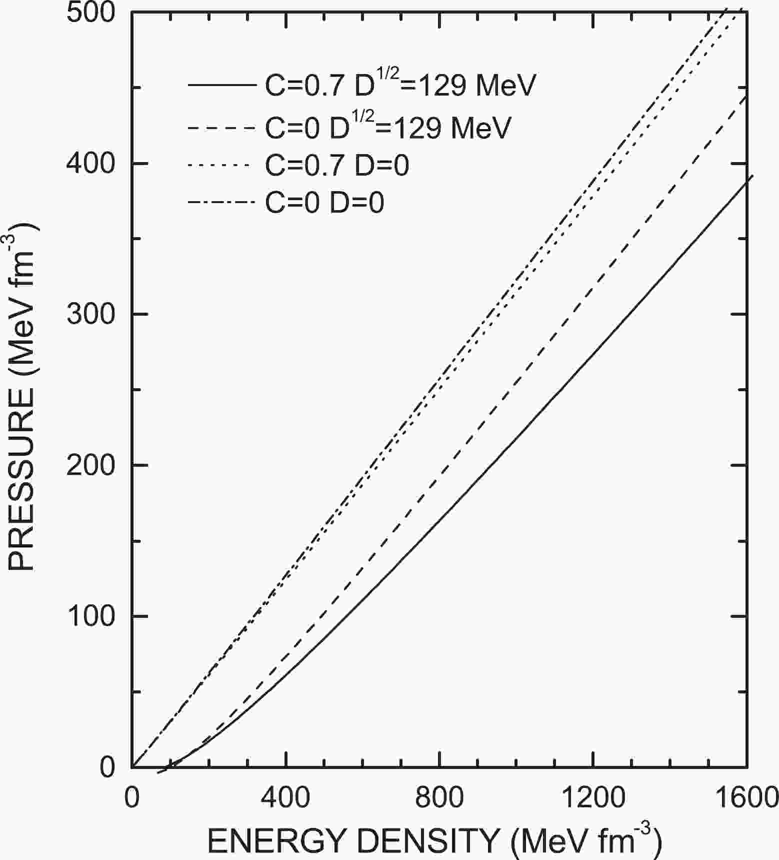
$ \rho_b $ , one can simultaneously solve Eqs. (8), (10), and (11) to obtain the values of effective chemical potentials$ \mu_i^*\ (i = u,d,s,e) $ . Then, according to Eqs. (12) and (13), the equation of state (EoS) of SQM can be obtained by$ P = P(E) $ .In Fig. 1, we present the EoS of SQM in the equivparticle model with the new quark mass scaling in Eq. (6). From this figure, one can readily find that the inclusion of interactions between quarks can significantly soften the EoS. Additionally, the effect of quark confinement (dashed line) prevails over that of perturbative interactions (dotted line) in the EoS with the specified model parameters.

Figure 1. EoS of SQM with new mass scaling in Eq. (6). From comparison of the solid line and dash-dotted line, it is obvious that the interactions between quarks can significantly soften the EoS.
-
In this section, employing a traditional method [26,50], we give the bulk viscosity of SQM in the equivparticle model. After reproducing the existing results [26], we investigate the effects of quark interactions on the bulk viscosity by adopting different mass scalings.
First, we assume that the volume per unit mass of SQM is
$ v $ , which, due to the vibration of a strange quark star, oscillates harmonically according to the following equation:$ v(t) = v_0+\Delta v\sin\left(\frac{2\pi t}{\tau}\right)\equiv v_0+\delta v(t), $

(14) where
$ \tau $ is the volume vibration period,$ v_0 $ is the equilibrium volume, and$ \Delta v $ is the vibration amplitude, which is small compared with$ v_0 $ , i.e.,$ \Delta v/v_0\ll1 $ . The vibration of$ v $ could result in the change in particle phase space and further cause variation in the particle number per unit mass,$ n_i(t) = n_{i0}+\delta n_i(t), $

(15) and unless otherwise stated,
$ i $ represents$ u, d, $ and$ s $ quarks here and below;$ \delta n_i $ can be obtained by integration:$ \delta n_d = -\delta n_s = \int_0^t\frac{{\rm d}n_d}{{\rm d}t}{\rm d}t. $

(16) As for the reaction rate
${\rm d}n_d/{\rm d}t$ , we adopt the result valid in low temperatures ($ T\ll\mu_i $ ) [26], i.e.,$ \frac{{\rm{d}} n_{d}}{{\rm d} t} \approx G_{C} \mu_{d}^{5} \delta \mu\left(\delta \mu^{2}+4 \pi^{2} T^{2}\right) v_{0}, $

(17) where
$ \delta\mu\equiv\mu_s-\mu_d $ , and the constant$ G_c $ is connected to the weak coupling$ G_F $ and the Cabibbo angle$ \theta_C $ by$ G_{{\rm{C}}} \equiv \frac{16}{5 \pi^{5}} G_{F}^{2} \sin ^{2} \theta_{C} \cos ^{2} \theta_{C} = 6.76 \times 10^{-26} {\rm{MeV}}^{-4}. $

(18) Because the bulk viscosity of SQM mainly stems from the nonleptonic weak reaction
$ u+d\leftrightarrow u+s $ , the pressure$ P $ can be expanded near the$ \beta $ -equilibrium pressure$ P_0 $ , i.e.,$ P(t) = P_0+\left(\frac{\partial P}{\partial v}\right)_0\delta v +\left(\frac{\partial P}{\partial n_d}\right)_0\delta n_d +\left(\frac{\partial P}{\partial n_s}\right)_0\delta n_s. $

(19) Then, the mean dissipation rate of the vibration energy per unit mass is given by
$ \left(\frac{{\rm{d}} w}{{\rm{d}} t}\right)_{{\rm{av}}} = -\frac{1}{\tau} \int_{0}^{\tau} P(t) \frac{{\rm{d}} v}{{\rm{d}} t} {\rm{d}} t. $

(20) In practice, the first two terms on the right-hand side of Eq. (19) do not contribute to energy dissipation in Eq. (20). Therefore, they can be safely ignored.
Similarly, the quark chemical potential difference
$ \delta\mu $ can also be expanded in terms of$ \delta v $ ,$ \delta n_d $ , and$ \delta n_s $ , namely$ \delta \mu(t) = \left(\frac{\partial \delta \mu}{\partial v}\right)_{0} \delta v +\left(\frac{\partial \delta \mu}{\partial n_{{\rm{d}}}}\right)_{0} \delta n_{{\rm{d}}}+\left(\frac{\partial \delta \mu}{\partial n_{{\rm{s}}}}\right)_{0} \delta n_{{\rm{s}}}, $

(21) in which
$ \displaystyle\frac{\partial\delta\mu}{\partial x} = \displaystyle\frac{\partial\mu_s}{\partial x} -\frac{\partial\mu_d}{\partial x},\ (x = v,n_d,{\rm{or}}\ n_s) $ . Importantly,$\displaystyle \frac{\partial\mu_i}{\partial v} $ is connected to the third and fourth terms in Eq. (19) by the following relation:$ \frac{\partial \mu_{i}}{\partial v} = -\frac{\partial P}{\partial n_{i}}. $

(22) To obtain the bulk viscosity, one should give the expressions of derivatives of chemical potentials in terms of
$ v $ ,$ n_d $ , and$ n_s $ . To this end, we start from the quark number per unit mass$ n_i $ ,$ n_i = \rho_iv = \frac{1}{\pi^2}(\mu_i^{*2}-m_i^2)^{3/2}v, $

(23) from which it is not difficult to obtain the differential form of
$ n_i $ , i.e.,$ {\rm d} n_{i} = v {\rm d} \rho_{i}+\rho_{i} {\rm d} v = \frac{3v\nu_i}{\pi^{2}}\left(\mu_{i}^{*} {\rm d} \mu_{i}^{*}-m_{i} {\rm d} m_{i}\right) +\rho_{i} {\rm d} v. $

(24) In the equivparticle model, to mimic the complicated strong interactions between quarks, the particle masses are taken as functions of baryon number density, i.e.,
$ m_i = m_i(\rho_b) $ , from which the differential form of$ m_i $ can be written as$ {\rm d} m_i = \frac{{\rm d} m_i}{{\rm d} \rho_b}{\rm d} \rho_b = \frac{{\rm d} m_I}{{\rm d}\rho_b}{\rm d} \rho_b. $

(25) According to the definition of baryon number density
$ \rho_b = \displaystyle\frac{1}{3}\sum\nolimits_i \rho_i $ , one can obtain$ v\rho_b = \displaystyle\frac{1}{3}\sum\nolimits_i v\rho_i = \displaystyle\frac{1}{3}\sum\nolimits_i n_i $ . Then, the corresponding differential form is${\rm d}(v\rho_b) = v{\rm d}\rho_b+\rho_b{\rm d}v = \displaystyle\frac{1}{3} \sum\nolimits_i {\rm d}n_i$ , from which$ {\rm d} \rho_{b} = \frac{1}{3v} \sum\limits_{i} {\rm d}n_{i}-\frac{\rho_{b}}{v} {\rm d} v. $

(26) Substituting Eqs. (25) and (26) into Eq. (24), one can obtain the differential form of the particle number per unit mass
${\rm d}n_i$ , i.e.,$ \begin{aligned}[b] {\rm d}n_i = & \frac{3v\nu_i\mu_i^*}{\pi^2}{\rm d}\mu_i^*-\frac{\nu_i m_i}{\pi^2} \frac{{\rm d}m_I}{{\rm d}\rho_b}\sum\limits_j{\rm d}n_j\\ & +\left(\rho_i+\frac{3\nu_im_i\rho_b}{\pi^2} \frac{{\rm d}m_I}{{\rm d}\rho_b}\right){\rm d}v,\\ \equiv & C_{1i}{\rm d}\mu_i^*+C_{2i}\sum\limits_j{\rm d}n_j+C_{3i}{\rm d}v, \end{aligned} $

(27) where we have changed the dummy index
$ i $ in Eq. (26) to$ j $ in Eq. (27) and introduced three notations to give a tighter form of this expression, i.e.,$ C_{1i} \equiv \frac{3v\nu_i\mu_i^*}{\pi^2}, $

(28) $ C_{2i} \equiv -\frac{\nu_i m_i}{\pi^2}\frac{{\rm d}m_I}{{\rm d}\rho_b}, $

(29) $ C_{3i} \equiv \rho_i+\frac{3\nu_im_i\rho_b}{\pi^2}\frac{{\rm d}m_I}{{\rm d}\rho_b}. $

(30) Note that the chemical potentials in Eq. (27) are effective ones, which should be linked to the real ones. To do this, we use the differential form of Eq. (7), i.e.,
$ {\rm d}\mu_i^* = {\rm d}\mu_i+{\rm d}\mu_I. $

(31) To facilitate the derivation of bulk viscosity of SQM in the equivparticle model,
$ \mu_I $ can be redefined as a new function$ f $ as follows,$ \mu_I = -\frac{1}{3}\frac{{\rm d}m_I}{{\rm d}\rho_b}\frac{\partial\Omega_0}{\partial m_I} \equiv f(\rho_b,m_i(\rho_b),\mu_i^*). $

(32) Accordingly, the differential form of
$ \mu_I $ is$ {\rm d}\mu_I = \left(\frac{\partial f}{\partial\rho_b}+\frac{{\rm d}m_I}{{\rm d}\rho_b} \sum\limits_j\frac{\partial f}{\partial m_j}\right){\rm d}\rho_b +\sum\limits_j\frac{\partial f}{\partial\mu_j^*}{\rm d}\mu_j^*. $

(33) Substituting Eqs. (33) and (26) into Eq. (31) and re-arranging the terms, one can write the explicit differential form of effective chemical potential
$ {\rm d}\mu_i^* $ as$ \begin{aligned}[b] {\rm d}\mu_i^* = & \frac{1}{1-\displaystyle\frac{\partial f}{\partial\mu_i^*}}\bigg[{\rm d}\mu_i+\left(\frac{\partial f}{\partial\rho_b} +\frac{{\rm d}m_I}{{\rm d}\rho_b}\sum\limits_j\frac{\partial f}{\partial m_j}\right) \left(\frac{1}{3v} \sum\limits_{j} {\rm d}n_{j}-\frac{\rho_{b}}{v} {\rm d} v\right)+\sum\limits_{j \neq i}\frac{\partial f}{\partial\mu_j^*}{\rm d}\mu_j^*\bigg],\\ =& \frac{1}{1-\displaystyle\frac{\partial f}{\partial\mu_i^*}}{\rm d}\mu_i+\frac{1}{3v} \frac{1}{1-\displaystyle\frac{\partial f}{\partial\mu_i^*}}\left(\frac{\partial f}{\partial\rho_b} +\frac{{\rm d}m_I}{{\rm d}\rho_b}\sum\limits_j\frac{\partial f}{\partial m_j}\right)\sum\limits_{j} {\rm d}n_{j} -\frac{\rho_b}{v}\frac{1}{1-\displaystyle\frac{\partial f}{\partial\mu_i^*}}\left(\frac{\partial f}{\partial\rho_b} +\frac{{\rm d}m_I}{{\rm d}\rho_b}\sum\limits_j\frac{\partial f}{\partial m_j}\right){\rm d}v\\ & +\sum\limits_{j \neq i}\frac{\partial f}{\partial\mu_j^*}{\rm d}\mu_j^*. \end{aligned} $

(34) By taking
$ \begin{aligned}[b] A_i = \frac{1}{1-\displaystyle\frac{\partial f}{\partial\mu_i^*}}, \quad B = \frac{\partial f}{\partial\rho_b} +\frac{{\rm d}m_I}{{\rm d}\rho_b}\sum\limits_j\frac{\partial f}{\partial m_j}, \end{aligned} $

with
$ \frac{\partial f}{\partial\mu_i^*} = -\frac{m_i\nu_i}{\pi^2}\frac{{\rm d}m_I}{{\rm d}\rho_b}, $

(35) $ \frac{\partial f}{\partial m_j} = \frac{g_j}{4\pi^2} \left(\mu_j^*\nu_j-3m_j^2\ln\frac{\mu_j+\nu_j}{m_j}\right), $

(36) $ \frac{\partial f}{\partial\rho_b} = -\frac{{\rm d}^2m_i}{3{\rm d}\rho_b^2} \sum\limits_j\frac{g_jm_j}{4\pi^2}\left[\mu_j^*\nu_j-m_j^2\ln\frac{\mu_j^*+\nu_j}{m_j}\right], $

(37) one can rewrite Eq. (34) as
$ {\rm d}\mu_i^* = A_i{\rm d}\mu_i+\frac{A_iB}{3v}\sum\limits_j{\rm d}n_j-\frac{\rho_bA_iB}{v}{\rm d}v+ \sum\limits_{j \neq i}\frac{\partial f}{\partial\mu_j^*}{\rm d}\mu_j^*. $

(38) Substituting Eq. (38) into Eq. (27) and applying
${\rm d}n_i = \sum\nolimits_j\delta_{ij}{\rm d}n_j$ , where$ \delta_{ij} $ is the Kronecker delta, one can obtain the differential form of the real chemical potential$ \begin{aligned}[b] {\rm d}\mu_i = & \sum\limits_j\left(\frac{\delta_{ij}-C_{2i}}{A_iC_{1i}}-\frac{B}{3v}\right){\rm d}n_j +\left(\frac{\rho_bB}{v}-\frac{C_{3i}}{A_iC_{1i}}\right){\rm d}v\\ &-\frac{1}{A_i}\sum\limits_{j \neq i}\frac{\partial f}{\partial\mu_j^*}{\rm d}\mu_j. \end{aligned} $

(39) From Eq. (39), we immediately obtain
$ \left(\frac{\partial\mu_i}{\partial n_j}\right)_0 = \frac{\delta_{ij}-C_{2i}}{A_iC_{1i}}-\frac{B}{3v}, $

(40) $ \left(\frac{\partial\mu_i}{\partial v}\right)_0 = \frac{\rho_bB}{v}-\frac{C_{3i}}{A_iC_{1i}}. $

(41) Substituting Eqs. (40) and (41) into Eq. (19) and ignoring the first two terms on the right-hand side of Eq. (19), one obtains the pressure contributing to the dissipation energy,
$ \begin{aligned}[b] P(t) = & \left(\frac{\partial P}{\partial n_d}\right)_0\delta n_d +\left(\frac{\partial P}{\partial n_s}\right)_0\delta n_s\\ =& \left(\frac{C_{3d}}{A_dC_{1d}}-\frac{C_{3s}}{A_sC_{1s}}\right) \int_0^t\frac{{\rm d}n_d}{{\rm d}t}{\rm d}t. \end{aligned} $

(42) The chemical potential difference
$ \delta\mu $ , accordingly, can be derived in a similar manner, namely$\begin{aligned}[b] \delta\mu(t) = & \left(\frac{\partial\delta\mu}{\partial v}\right)_0\delta v +\left(\frac{\partial\delta\mu}{\partial n_d}\right)_0\delta n_d+ \left(\frac{\partial\delta\mu}{\partial n_s}\right)_0\delta n_s,\\ = &\left(\frac{C_{3d}}{A_dC_{1d}}-\frac{C_{3s}}{A_sC_{1s}}\right)\Delta v\sin(\omega t)\\ &-\left(\frac{1}{A_dC_{1d}}+\frac{1}{A_sC_{1s}}\right)\int_0^t\frac{{\rm d}n_d}{{\rm d}t}{\rm d}t,\end{aligned} $

(43) which naturally gives the differential equation of
$ \delta\mu(t) $ ,$ \begin{aligned}[b] \frac{{\rm d}\delta\mu(t)}{{\rm d}t} = & \left(\frac{C_{3d}}{A_dC_{1d}}-\frac{C_{3s}}{A_sC_{1s}}\right) \frac{2\pi\Delta v}{\tau}\cos\left(\frac{2\pi t}{\tau}\right)\\ & -\left(\frac{1}{A_dC_{1d}}+\frac{1}{A_sC_{1s}}\right)\frac{{\rm d}n_d}{{\rm d}t}. \end{aligned} $

(44) To solve this differential equation numerically, the related expressions of these notations in Eq. (44) are explicitly given as follows:
$ C_{3i} = \rho_i+\frac{3\nu_im_i\rho_b}{\pi^2}\frac{{\rm d}m_I}{{\rm d}\rho_b}, $

(45) $ \frac{1}{A_iC_{1i}} = \frac{1}{3v\mu_i^*} \left(\frac{\pi^2}{\nu_i}+m_i\frac{{\rm d}m_I}{{\rm d}\rho_b}\right). $

(46) From these expressions, we can clearly see the mass-density dependent term
${\rm d}m_I/{\rm d}\rho_b$ , which explicitly denotes the main feature of the bulk viscosity in the equivparticle model.The mean dissipation rate of the vibration energy per unit mass reads
$\begin{aligned}[b] \left(\frac{{\rm d}w}{{\rm d}t}\right)_{\rm{av}} = & -\frac{1}{\tau}\int_0^\tau P(t)\frac{{\rm d}v}{{\rm d}t}{\rm d}t\\ =& \frac{\Delta v}{\tau}\frac{2\pi}{\tau} \left(\frac{C_{3s}}{A_sC_{1s}}-\frac{C_{3d}}{A_dC_{1d}}\right) \\ &\times\int_0^\tau {\rm d}t \left(\int_0^t\frac{{\rm d}n_d}{{\rm d}t}{\rm d}t\right)\cos\left(\frac{2\pi t}{\tau}\right). \end{aligned} $

(47) Finally, the bulk viscosity is
$\begin{aligned}[b] \zeta \equiv & 2\frac{({\rm d}w/{\rm d}t)_{\rm{av}}}{v_0} \left(\frac{v_0}{\Delta v}\right)^2\left(\frac{\tau}{2\pi}\right)^2\\ =& \frac{1}{\pi}\frac{v_0}{\Delta v} \left(\frac{C_{3s}}{A_sC_{1s}}-\frac{C_{3d}}{A_dC_{1d}}\right) \\ & \times \int_0^\tau {\rm d}t \left(\int_0^t\frac{{\rm d}n_d}{{\rm d}t}{\rm d}t\right)\cos\left(\frac{2\pi t}{\tau}\right). \end{aligned} $

(48) Due to the cubic term of
$ \delta\mu $ ($ \delta\mu \lesssim 0.1 $ MeV) in Eq. (17), it is not possible to solve the bulk viscosity analytically. However, in the relatively high-temperature limit ($ 2\pi T\gg\delta\mu $ , or the temperature of interest here satisfies$ T \lesssim 1\ {\rm{MeV}} $ ), one can ignore the cubic term and find the analytical form of bulk viscosity as$ \zeta_a = \frac{\alpha T^2}{\omega^{2}+\beta T^4}\left[1-\left(1-{\rm e}^{-\beta^{1/2} T^2 \tau}\right) \frac{2 \beta^{1/2} T^2/ \tau}{\omega^{2}+\beta T^4}\right], $

(49) where
$ \alpha = G_{c} \mu_{d}^{5} v_{0}^{2} 4 \pi^{2} \left(\frac{C_{3d}}{A_{d} C_{1 d}} -\frac{C_{3 s}}{A_{s} C_{1 s}}\right)^{2}, $

(50) and
$ \beta = G_{c}^2 \mu_{d}^{10} v_{0}^2 16 \pi^{4} \left(\frac{1}{A_{d} C_{1d}}+\frac{1}{A_{s} C_{1s}}\right)^2. $

(51) In what follows, to prove the validity of our results, we show that in the mass-density-independent case, i.e., parameters
$ C = D = 0 $ , the equations in our model are exactly the same as those in the bag model. If$ C = D = 0 $ ,$ A_i, B, C_{1i}, C_{2i} $ , and$ C_{3i} $ can be respectively simplified to$ A_i = 1, B = 0, C_{1i} = \frac{3v\nu_i\mu_i}{\pi^2}, C_{2i} = 0, C_{3i} = \rho_i. $

(52) Accordingly, Eq. (40) and Eq. (41) can be reduced to
$ \left(\frac{\partial\mu_i}{\partial n_j}\right)_0 = \frac{\delta_{ij}\pi^2}{3v\nu_i\mu_i} $

(53) and
$ \left(\frac{\partial\mu_i}{\partial v}\right)_0 = -\frac{\pi^2\rho_i}{3v\nu_i\mu_i}. $

(54) Therefore, Eq. (39) can be simplified to
$ {\rm d}\mu_i = \frac{\pi^2}{3v\nu_i\mu_i}{\rm d}n_i-\frac{\pi^2\rho_i}{3v\nu_i\mu_i}{\rm d}v = \frac{\pi^2}{3\nu_i\mu_i}{\rm d}\rho_i, $

(55) which is exactly the same as the differential form of the particle number density
$ \rho_i = \dfrac{\nu_i^3}{\pi^2} $ , where$ \nu_i = \sqrt{\mu_i^2-m_i^2} $ with the real chemical potential$ \mu_i $ . In this case, the bulk viscosity in the equivparticle model given by Eq. (48) is reduced to$ \zeta = -\frac{1}{\pi}\frac{v_0}{\Delta v}\frac{m_s^2}{3v_0\mu_d} \int_0^\tau {\rm d}t\left(\int_0^t\frac{{\rm d}n_d}{{\rm d}t}{\rm d}t\right)\cos\left(\frac{2\pi t}{\tau}\right). $

(56) Meanwhile, although the analytical form of
$ \zeta $ in Eq. (49) is not changed,$ \alpha $ and$ \beta $ are respectively reduced to$ \alpha = \frac{4\pi^2}{9}G_c\mu_d^3 m^4_{s0}, $

(57) and
$ \beta = \frac{64\pi^8}{9}G_c^2\mu_d^6\left(1+\frac{m_{s0}^2}{4\mu_d^2}\right)^2. $

(58) They are respectively consistent with Eqs. (15-18) in Ref. [26]. This limiting case suggests that the bulk viscosity in the equivparticle model can be treated as a generalization of previous results in the bag model.
-
To calculate the bulk viscosity of SQM in the equivparticle model, one should first give the EoS of SQM and then simultaneously solve Eqs. (17), (44), and (48) numerically.
In Fig. 2, we show the behavior of the bulk viscosity
$ \zeta $ as function of relative volume perturbation amplitude$ \Delta v/v_0 $ and temperature$ T $ . The lines with solid balls calculated by Eq. (48) show the results in the equivparticle model, while the lines with stars calculated by Eq. (56) indicate the bulk viscosity results in the mass-density-independent case, which are exactly the same as the previous results in the bag model [26]. In the equivparticle model, the parameters$ C $ and$ D^{1/2} $ in mass scaling Eq. (6) are respectively taken as 0.7 and 129 MeV, which guarantees that the EoS of SQM can support quark stars with maximum mass larger than 2$ {\rm M}_\odot $ , and that the SQM is absolutely stable. In addition, temperatures are given as$ 10^{-5} $ ,$ 10^{-3} $ , and$ 10^{-1} $ MeV, denoted by red, green, and blue lines, respectively.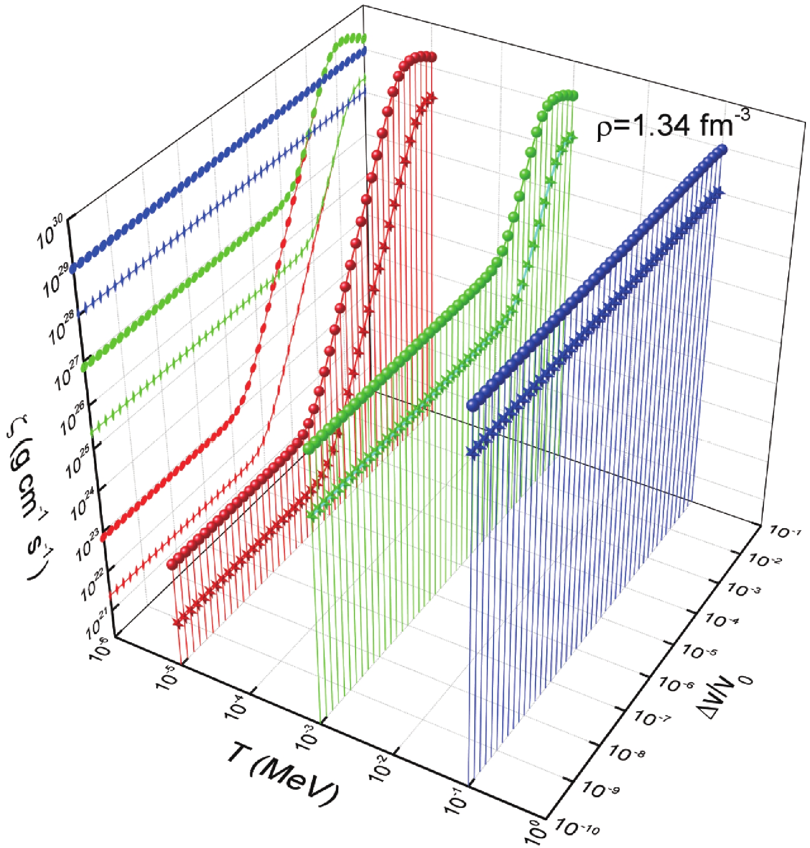
Figure 2. (color online) Bulk viscosity as a function of relative volume perturbation amplitude and temperature. The lines with solid balls and stars indicate the results in the equivparticle model and the mass-density-independent case (i.e., the bag model), respectively. In numerical calculations, the oscillation period of quark matter is
$ \tau = 10^{-3} $ s, and the temperatures$ T $ are$ 10^{-5} $ ,$ 10^{-3} $ , and$ 10^{-1} $ MeV, denoted by red, green, and blue lines, respectively.In numerical calculations, the baryon number density is set to
$ \rho = 1.34 $ fm-3. To facilitate comparison of the magnitude of bulk viscosity, we also give the projection of each line on the$ Z-Y $ plane. From Fig. 2, it is clear to see that at different temperatures, the bulk viscosity in the equivparticle model is generally larger than that in the bag model by a magnitude of approximately 2 orders. This is not difficult to understand according to the conclusion we obtained in our previous paper [45] that the inclusion of interactions between quarks can significantly enhance the bulk viscosity of SQM. To better understand this aspect, we introduce a parameter$ \kappa $ in the interaction part of mass scaling, i.e.,$ m_i = m_{i0}+\kappa m_I,\ \kappa\in[0,1]. $

(59) If
$ \kappa = 0 $ , the interactions between quarks vanishes; while$ \kappa $ approaches unity, the interactions are gradually recovered.Figure 3 reveals the interaction intensity behavior of the bulk viscosity, from which one can observe that as interactions between quarks become strong, the bulk viscosity becomes large as well. Whether we ignore the quark confinement effects (
$ D = 0 $ , dashed line) or the perturbative interactions ($ C = 0 $ , dotted line), this behavior still holds. From Fig. 3, it is also clearly indicated that the quark confinement effects have a more important influence on the bulk viscosity than the perturbative interactions. This conclusion still holds if we adopt other values of parameter sets, where the approximate relation between$ C $ and$ D $ in the absolutely stable region of SQM [46] is given as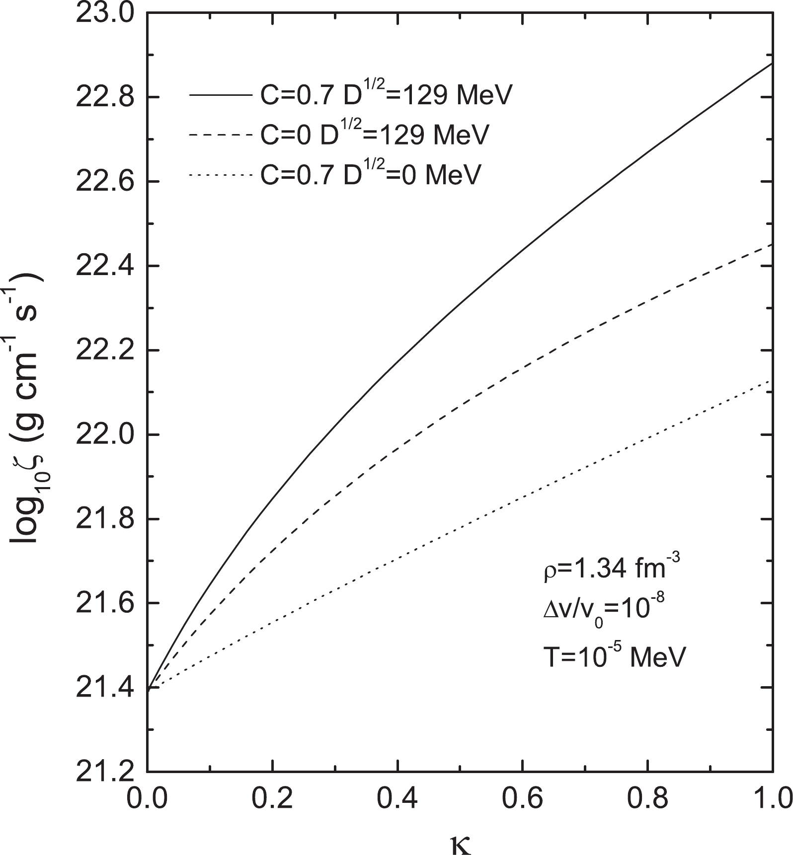
Figure 3. Interaction intensity behavior of bulk viscosity. As the interactions between quarks become strong, the bulk viscosity becomes large. In numerical calculations, all the parameter values are the same as in Fig. 2. In addition, the values of
$ \Delta v/v_0 $ and$ T $ are set to$ 10^{-8} $ and$ 10^{-5} $ MeV, respectively.$ D^{1/2}/{\rm{MeV}} = \left\{\begin{array}{ll} -48C+156, & C\in[-0.5,0],\\ -\displaystyle\frac{27}{0.7}C+156, & C\in(0,0.7]. \end{array}\right. $

This relation is adopted in Fig. 4 on the top and bottom X-axes. To study the perturbative interactions on the bulk viscosity, we set
$ D = 0 $ , and the results are given by the dotted line. Similarly, to study the confinement interactions on the bulk viscosity, we set$ C = 0 $ , and the results are given by the dashed line. From these two lines, it is observed that with increasing$ C $ or$ D $ , the bulk viscosity increases. Furthermore, in a large parameter range of$ C $ and$ D $ , it is shown again that the confinement effects on the bulk viscosity are much larger than the perturbative interactions. For the purpose of comparison, we also present the bulk viscosity of SQM with both confinements effects and perturbative interactions, shown by the solid line.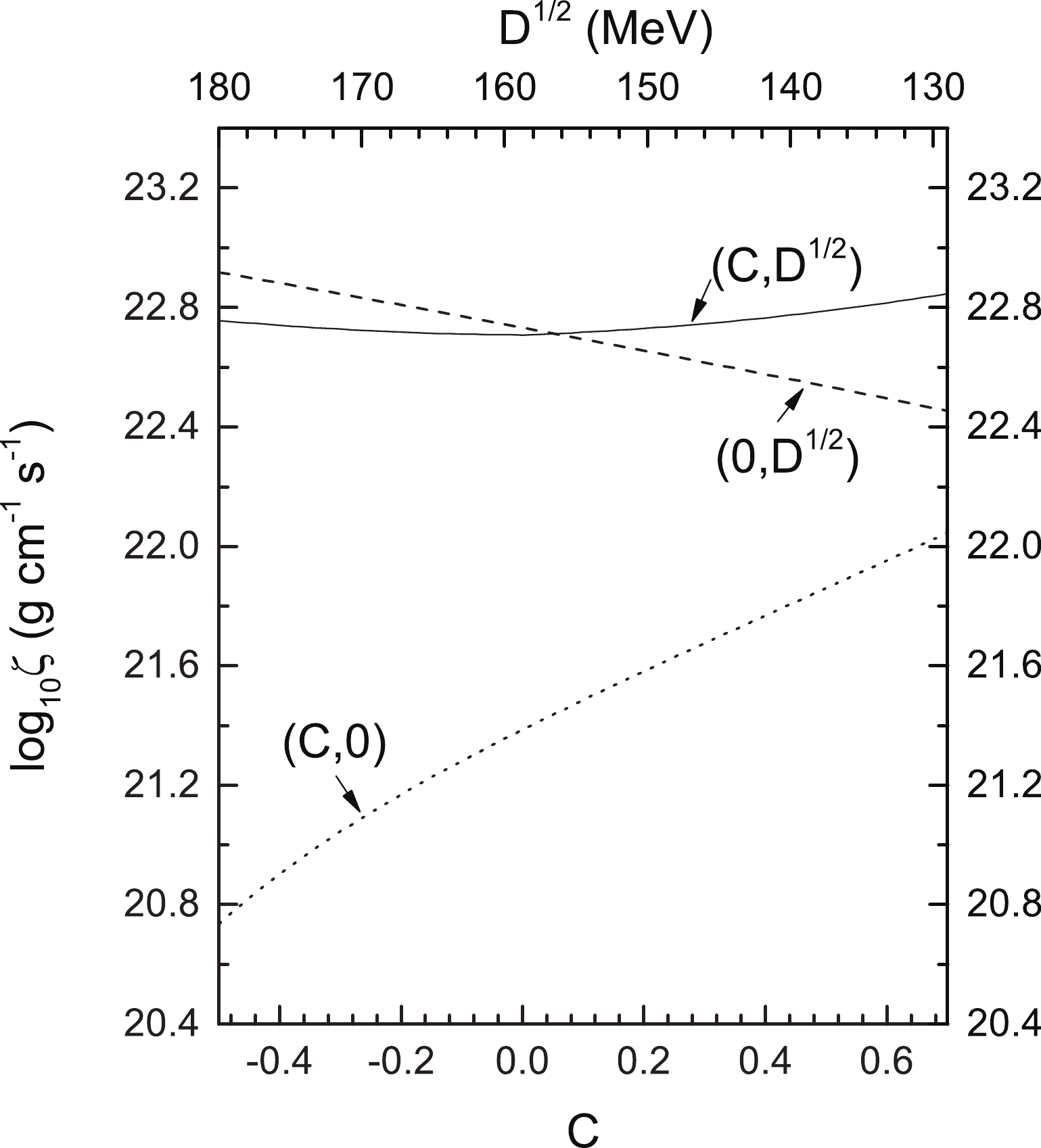
Figure 4. Different interactions with bulk viscosity of absolutely stable SQM. From the dashed and dotted lines, it is shown that the confinement effects from model parameter
$ D $ contribute to the bulk viscosity much more than the perturbative interactions from model parameter$ C $ .To explicitly show the effects of quark confinement and perturbative interactions on the bulk viscosity, in Fig. 5 we present the bulk viscosity of SQM adopting various model parameters
$ C $ and$ D $ . If$ C $ and$ D $ both vanish, it corresponds to the bag model predictions (the dash-dotted line). If only the perturbative interactions are accounted for, we obtain the results indicated by the dotted line, which are much higher than those of the bag model. Moreover, if only the quark confinement effects are included, the results are given by the dashed line, which is consistent with the implications of Fig. 3, namely that the quark confinement effects prevail over the perturbative interactions in the bulk viscosity of SQM. Finally, as expected, if these two types of interactions are both considered, the bulk viscosity shown by the solid line becomes the highest. It is interesting to note that the results shown by the dashed line are almost the same as those shown by the solid line at large volume vibration amplitudes, which suggests that the perturbative interactions become insignificant in comparison.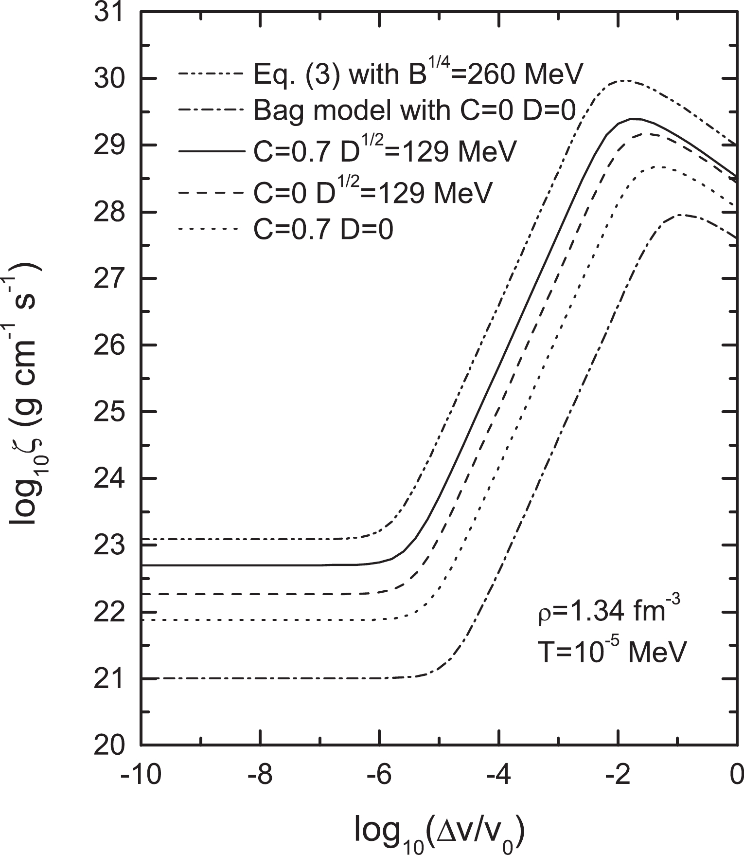
Figure 5. Effects of interactions between quarks on the bulk viscosity of SQM. The solid line gives the results in the equivparticle model, whereas the dash-dotted line corresponds to those in the bag model. The dotted line only includes the perturbative interactions, and the dashed line only includes the quark confinement effects. To verify the impact of different mass scaling on bulk viscosity, we also give the results calculated for the equivparticle model with mass scaling in Eq. (3).
To study the influence of different mass scaling on bulk viscosity, we adopt the mass scaling in Eq. (3), which gives the largest bulk viscosity. However, we should emphasize that this situation does not contradict our conclusion, as the mass scaling in Eq. (3) can provide much stronger quark confinement effects.
Customarily, strange stars have strong magnetic fields, which have a significant influence on the transport coefficients, especially the bulk viscosity. In Ref. [34], the authors investigated the bulk viscosity in greater detail, and found that in strong magnetic fields, the transport coefficients of SQM become anisotropic. However, for the magnetic fields
$ B<10^{17} $ G, the effect of magnetic field on bulk viscosity can be ignored, and a comparison with our results at the low-B limit is possible. In Fig. 6, we show the results of the bulk viscosity from Ref. [34] and the equivparticle model at the same baryon number density$ \rho \sim 0.787 $ fm-3 (or$ \mu_u = \mu_d = 400 $ MeV in Ref. [34]). From Fig. 6, we find that the bulk viscosity in our model is usually higher than that in Ref. [34], except for$ 10 \lesssim \omega/{\rm{s}}^{-1} \lesssim 1000 $ , where$ \omega = 2\pi/\tau $ . In addition, with increasing$ \omega $ , the bulk viscosity in the equivparticle model decreases much more slowly, because the interactions between quarks are considered.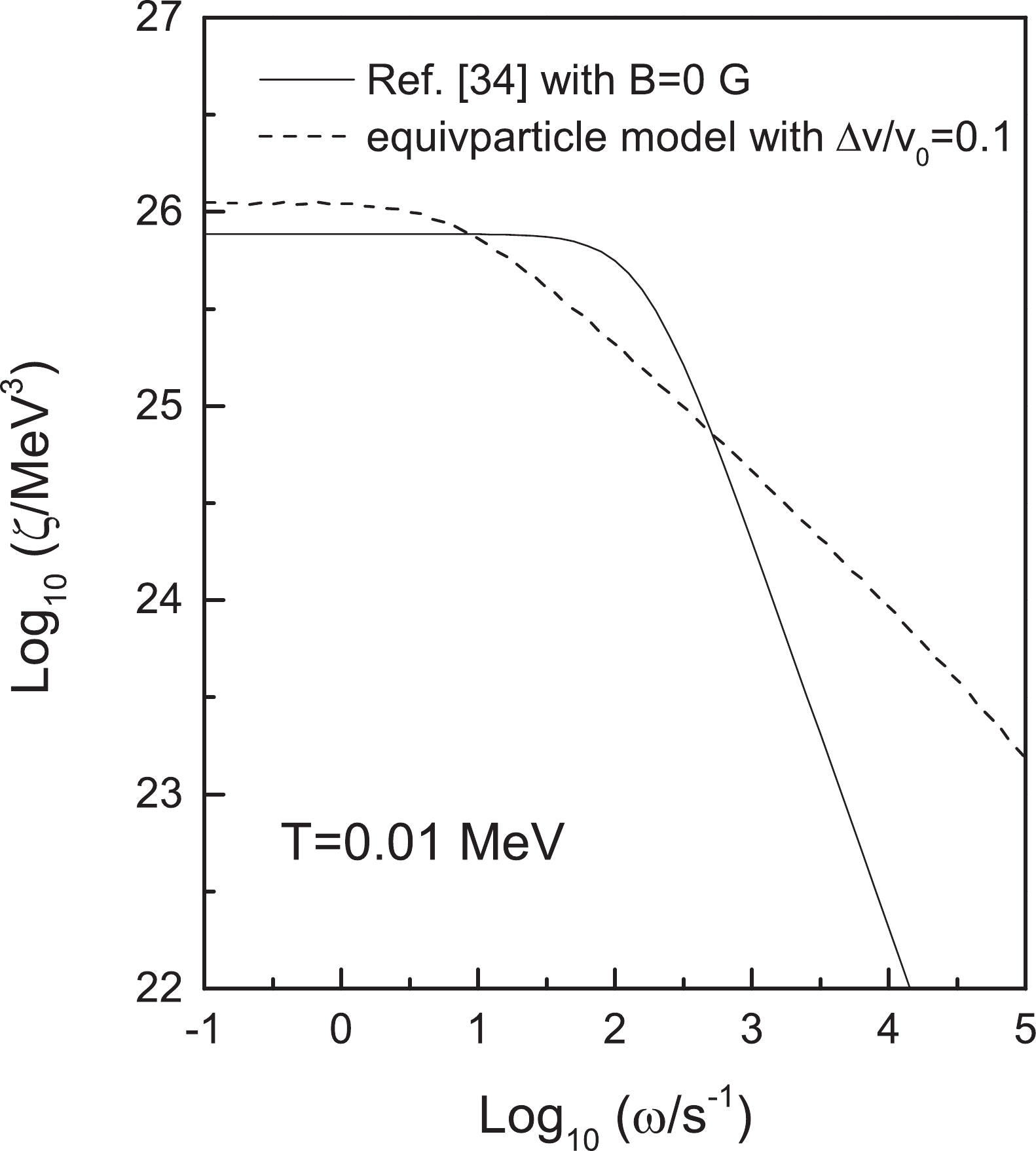
Figure 6. Comparison of the bulk viscosity in Ref. [34] and equivparticle model at the same baryon number density
$ \rho \sim 0.787 $ fm−3.To understand how the interactions between quarks can enhance the bulk viscosity of SQM, we give the time behavior of quark chemical difference
$ \delta\mu = \mu_s-\mu_d $ with different$ \Delta v/v_0 $ in Fig. 7. In these panels, from top to bottom,$ \Delta v/v_0 $ values are$ 10^{-1} $ ,$ 10^{-2} $ , and$ 10^{-3} $ , respectively. The solid lines represent the results including interactions between quarks with$ C = 0.7 $ and$ D^{1/2} = 129 $ MeV, whereas the dashed lines give the results with vanishing$ C $ and$ D $ . It can be seen from Fig. 7 that with increasing$ \Delta v/v_0 $ , the amplitudes of$ \delta\mu $ in both cases become large. Furthermore, according to Fig. 7, the amplitudes are significantly enhanced once the interactions between quarks are considered, which suggests that more energy could be involved in one period of oscillation and physically means a larger bulk viscosity of SQM.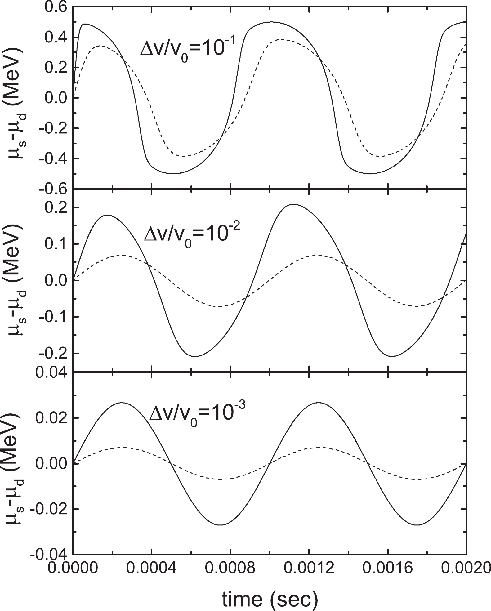
Figure 7.
$ \delta\mu(t) $ for two cycles with parameters$ \rho_b = 1.34 $ fm−3,$ T = 10^{-5} $ MeV, and$ \tau = 10^{-3} $ s and$ \Delta v/v_0 = 10^{-1}, 10^{-2},\; {\rm{and}}\;\ 10^{-3} $ , respectively. The solid lines indicate the results in the equivparticle model with parameters$ C\! = 0.7 $ and$ D^{1/2} = 129 $ MeV, whereas the dashed lines correspond to the results with$ C\! =\! D \!=\! 0 $ .A situation similar to that of the amplitude of
$ \delta\mu $ in Fig. 7 can be observed in Table 1, which gives the mean dissipation rate of vibration energy per unit volume$\dfrac{1}{v_0}\left(\dfrac{{\rm d}w}{{\rm d}t}\right)_{av}$ . The corresponding value reflects how much energy can be dissipated during one period of oscillation per unit volume. From Table 1, one can find that when the interactions between quarks are considered and$ \Delta v/v_0 $ is relatively large, the dissipation rate is very high, which implies that large amplitude oscillations in a quark star do not last. Contrary to the large amplitude oscillation case, small amplitude oscillation usually persists for a long time. In fact, the damping time of large amplitude oscillations can be shorter than one millisecond, while small amplitude oscillations can last for years [26,45]. In the next section, the oscillation damping times for strange stars are also investigated, which are in accordance with the conclusion obtained here.$ \Delta v/v_0 $ 

$ 10^{-1} $ 

$ 10^{-2} $ 

$ 10^{-3} $ 

$ (C,D^{1/2}/ {\rm{MeV}})$ 

(0.7, 129) (0, 0) (0.7, 129) (0, 0) (0.7, 129) (0, 0) $\dfrac{1}{v_0}\left(\dfrac{{\rm d}w}{{\rm d}t}\right)_{av}$ 

3.626×10¹³ 4.608×10¹² 6.599×10¹¹ 4.877×10⁹ 1.955×10⁸ 4.926×10⁵ Table 1. Mean dissipation rate of vibration energy per unit volume
$\dfrac{1}{v_0}\left(\dfrac{{\rm d}w}{{\rm d}t}\right)_{av}$ in units of g·fm−3·s−1 as functions of model parameters$ (C,D^{1/2}) $ and relative amplitude of vibration$ \Delta v/v_0 $ . Other model parameters are the same as in Fig. 7.In what follows, we aim to find the reasonable ranges of relative oscillation amplitude
$ \dfrac{\Delta v}{v_0} $ and temperature$ T $ for the analytical expression of bulk viscosity given in Eq. (49). For this purpose, we define a new function$ \Theta $ ,$ \Theta = \frac{\zeta-\zeta_a}{\zeta}, $

(60) which reflects the accuracy of
$ \zeta_a $ compared to$ \zeta $ .In Fig. 8,
$ \Theta $ is given as a function of$ \dfrac{\Delta v}{v_0} $ and$ T $ , and two isolines of$ \Theta $ are shown with values of$ 10^{-1} $ (solid line) and$ 10^{-2} $ (dashed line), respectively. From this figure, it is not difficult to conclude that when the accuracy$ \Theta = 10^{-1} $ , the relation between$ \dfrac{\Delta v}{v_0} $ and$ T $ can be approximately written as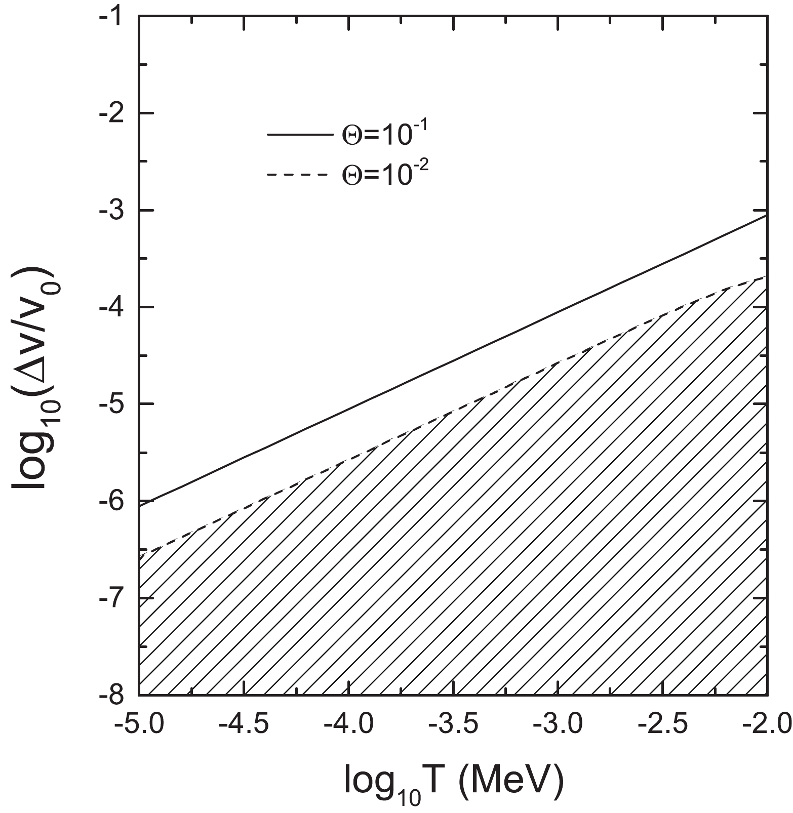
Figure 8.
$ \Theta $ as a function of relative oscillation amplitude$ \frac{\Delta v}{v_0} $ and temperature$ T $ . Two isolines of$ \Theta $ are shown, with values of$ 10^{-1} $ (solid line) and$ 10^{-2} $ (dashed line), respectively.$ \log_{10}\bigg(\frac{\Delta v}{v_0}\bigg)\approx\log_{10}T/\mathrm{MeV}-1 \quad (\Theta = 10^{-1}, T\lesssim 10^{-2}\ {\rm{MeV}}), $

(61) and when
$ \Theta = 10^{-2} $ , the relation should be changed to$ \log_{10}\bigg(\frac{\Delta v}{v_0}\bigg)\approx\log_{10}T/\mathrm{MeV}-1.5 \quad (\Theta = 10^{-2}, T\lesssim10^{-2}\ {\rm{MeV}}). $

(62) In fact, in the enhanced perturbative QCD model studied in Ref. [45], we had derived the similar relation between
${\Delta v}/{v_0}$ and$ T $ given by Eq. (61). Here, we obtain it again in a more visualized way in the equivparticle model. Furthermore, we update this relation when the accuracy is improved to$ 10^{-2} $ . Additionally, the shaded area in Fig. 8 gives the ranges of parameters${\Delta v}/{v_0}$ and$ T $ corresponding to$ \Theta $ with accuracy higher than$ 10^{-2} $ . Here, we should point out that the relations given in Eqs. (61) and (62) are not only valid in the current employed model but also reasonable in other phenomenological models, for example, the bag model, quasiparticle model, or perturbative model. -
Given the EoS of quark matter in the equivparticle model, one can obtain the properties of strange quark stars by numerically solving the following Tolman-Oppenheimer-Volkov (TOV) equation:
$ \frac{{\rm{d}} P}{{\rm{d}} r} = -\frac{G m E}{r^{2}} \frac{(1+P / E)\left(1+4 \pi r^{3} P / m\right)}{1-2 G m / r}, $

(63) with the subsidiary condition
$ \frac{{\rm{d}} m}{{\rm{d}} r} = 4 \pi r^{2} E, $

(64) where
$ G = 6.707 \times 10^{-45} {\rm{MeV}}^{ -2} $ is the gravitational constant.In Fig. 9, we give the mass-radius relations of quark stars with model parameter sets
$(C,D^{1/2}/{\rm{MeV}}) =$ (0.7, 129) and (0, 129), respectively. As we can see from the figure, the maximum mass (denoted by solid dots) of a quark star can be larger than 2${\rm M}_\odot$ , which now is generally taken as a popular constraint on the EoS of SQM [51-53]. When model parameter$ D = 0 $ , it can be seen from Fig. 1 that the pressure vanishes when the energy density becomes zero, which corresponds to zero particle number density. However, as is well established, strange stars have nonzero surface quark number density. Therefore, for$ D = 0 $ the surface pressure of strange stars is positive, which implies strange stars would fall apart. Therefore, we do not give the mass-radius relation for$ D = 0 $ in Fig. 9. Alternatively, in our model with$ D = 0 $ , SQM only exists in the interior of neutron stars or hybrid stars with nuclear matter covering the surfaces of compact stars. This can also be understood from the mass scaling in Eq. (6), which does not satisfy the basic quark confinement in QCD if$ D = 0 $ .
Figure 9. Mass-radius relations for strange stars. When model parameter
$ D = 0 $ , the requirement of quark confinement cannot be satisfied, and there is no minus pressure in the EoS. Therefore, the mass-radius relations are not given in this figure for$ D = 0 $ .In Fig. 10, the density profiles for different model parameter sets
$ (C,D^{1/2}/{\rm{MeV}}) = (0.7,129) $ and$ (0,129) $ are given, in which the solid lines correspond to the most massive strange star, the dashed lines are for stars with canonical 1.4${\rm M}_\odot$ , and the dotted lines represent low-mass strange quark stars with unit solar mass. Additionally, the horizontal dash-dotted lines in both panels give the surface densities for these two cases. The intersection points of lines and the left axis denote the central densities, from which one can observe that the heavier the star is, the larger the difference in densities between the center and surface can be. In other words, the density distributions become more isotropic for less massive stars. Therefore, it is reasonable to take approximately constant values for low-mass star densities [54]. For more information, one can refer to Table 2, in which values of typical parameters of stars are tabulated. In such cases, the damping time$ \tau_D $ of quark stars can be calculated by$ (C,D^{1/2}/{\rm{MeV}}) $ 

$ M/M_\odot $ 

$ R $ /km

$ \rho_c $ /fm−3

$ \rho_s $ /fm−3

$ \bar{\rho} $ /fm−3

2.13 13.71 0.649 0.089 0.234 (0.7,129) 1.4 14.38 0.215 0.089 0.134 1 13.40 0.169 0.089 0.118 2.38 14.12 0.719 0.129 0.240 (0,129) 1.4 14.12 0.243 0.129 0.141 1 12.98 0.204 0.129 0.130 Table 2. Characteristic quantities for strange stars with typical model parameter sets
$ (C,D^{1/2}/{\rm{MeV}}) = (0.7,129) $ and$ (0,129) $ . The second through sixth columns give the maximum mass$ M $ , radius corresponding to maximum mass$ R $ , center baryon number density$ \rho_c $ , surface baryon number density$ \rho_s $ , and mean baryon number density$ \bar{\rho} $ , respectively.
Figure 10. Density profile for different model parameters
$ C $ and$ D $ . The solid line corresponds to the most massive quark star, the dashed line denotes the quark star with 1.4${\rm M}_\odot$ , the dotted line gives the star with 1${\rm M}_\odot$ , and the dash-dotted line shows the surface baryon number density of strange quark stars.$ \tau_D = 30^{-1}\bar{\rho}R^2\zeta^{-1}. $

(65) Employing the values of radius and mean density in Table 2, one can easily obtain the damping times for strange stars with canonical 1.4
${\rm M}_\odot$ , and the results are graphically given in Fig. 11.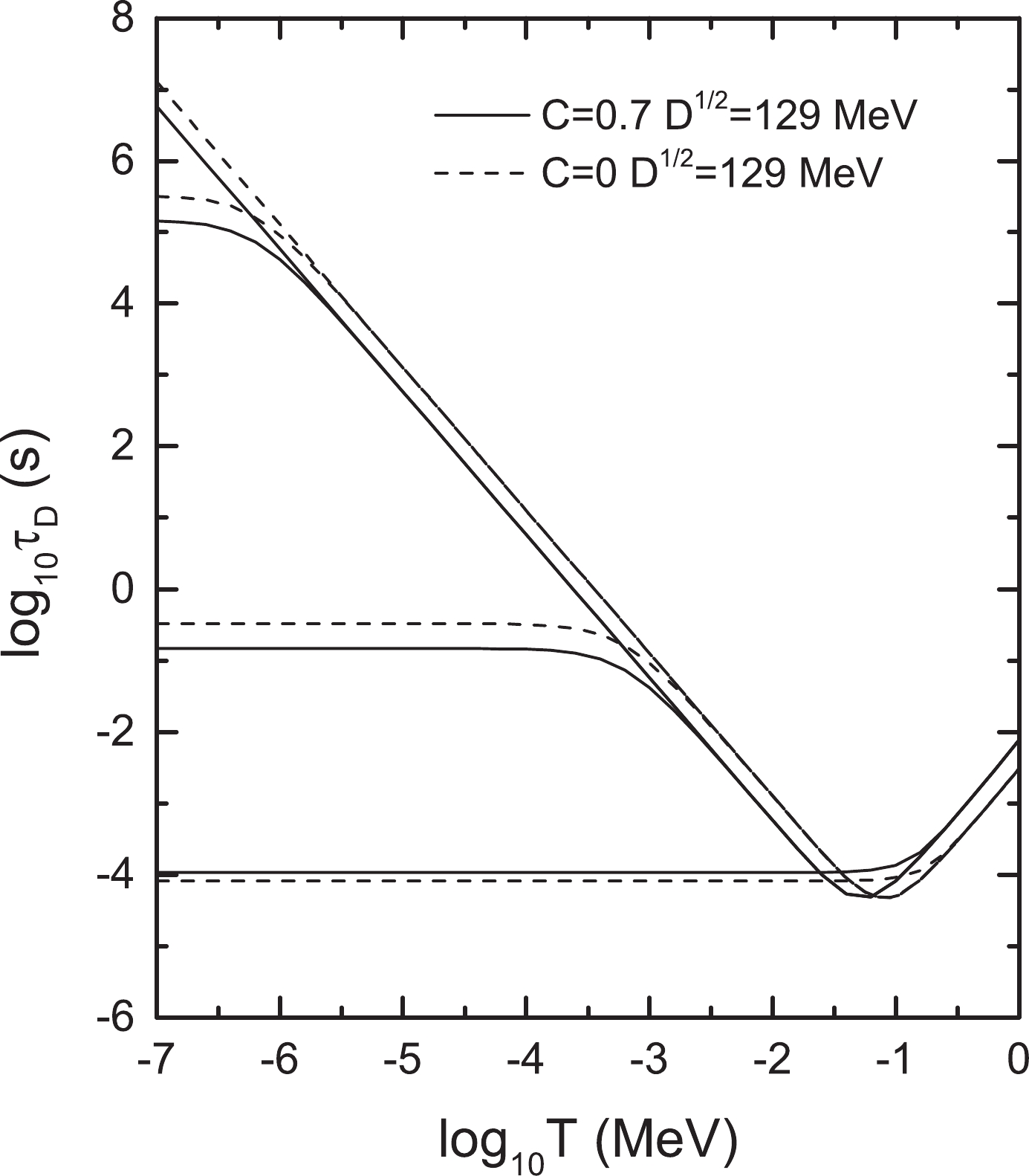
Figure 11. Damping times for quark stars with canonical 1.4 solar mass. From bottom to top, the relative oscillation amplitudes are
$ \Delta v/v_0 = 10^{-1} $ ,$ 10^{-4} $ ,$ 10^{-7} $ , and$ 10^{-10} $ , respectively, for both the solid and dashed lines.From this figure, it can be seen that the damping time with nonzero
$ C $ is a little shorter than that in the other case, except for large relative oscillation amplitudes, e.g.,$ \Delta v/v_0 = 10^{-1} $ , with damping times as short as approximately$ 10^{-4} $ s. In such cases, if a low-mass strange star experiences a strong starquake, the radial oscillations could be rapidly damped with the star heated by the release of the oscillation energy, which may have profound implications in astrophysics and affect the dynamics of the compact star merger [55-58]. -
We now investigate the
$ r $ -mode instability window for strange quark stars based on the obtained bulk viscosity. Driven by gravitational wave emission, a compact star experiences$ r $ -mode instability if its spin frequency exceeds one critical value [4,7] that is subject to various dissipation mechanisms, such as the bulk and shear viscosity. Therefore, the$ r $ -mode instability window is the consequence of competition between gravitational radiation and various damping mechanisms.For a given stellar configuration, the critical rotation frequency, as a function of temperature, is determined by the following equation:
$ \frac{1}{\tau} = \frac{1}{\tau_{\rm{gw}}}+\frac{1}{\tau_{\rm{sv}}}+\frac{1}{\tau_{\rm{bv}}}+\cdots = 0, $

(66) where
$ \tau_{\rm{gw}} $ is the characteristic time scale due to GW emission,$ \tau_{\rm{sv}} $ and$ \tau_{\rm{bv}} $ are damping time scales due to shear and bulk viscosities, respectively, and the ellipsis denotes other dissipation mechanisms, such as surface rubbing, which plays a crucial role in determining the$ r $ -mode instability window of neutron stars [59,60] and color-flavor-locked strange stars [21,54].To a very good approximation, the resulting bulk viscosity of SQM in the equivparticle model, according to the analytical form of bulk viscosity in Eq. (49), is given by
$ \zeta = \frac{\alpha T^2}{(\kappa\Omega)^2+\beta T^4}. $

(67) Here
$ \kappa = 2/3 $ is for dominant$ r $ mode, and$ \Omega $ is angular rotation frequency. Here,$ \alpha $ and$ \beta $ can be rewritten in cgs units as$ \alpha = 9.39\times10^{22}\mu_d^5\left(\frac{3C_{3d}v_0}{A_dC_{1d}}-\frac{3C_{3s}v_0}{A_sC_{1s}}\right)^2 \ ({\rm{g}}\cdot {\rm{cm}}^{-1}\cdot {\rm{s}}^{-1}), $

(68) and
$ \beta = 7.11\times10^{-4}\left[\frac{3\mu_d^5v_0}{2\pi^2} \left(\frac{1}{A_dC_{1d}}+\frac{1}{A_sC_{1s}}\right)\right]^2 \ ({\rm{s}}^{-2}). $

(69) In analogy to previous results of
$ \zeta $ in Refs. [26,44], a low-$ T $ limit of$ \zeta $ in cgs units yields$ \zeta^{{\rm{low}}}\approx\bar{\zeta}^{{\rm{low}}}\bar{\rho} T^2(\kappa\Omega)^{-2}m_{100}^4, $

(70) with
$ \bar{\zeta}^{{\rm{low}}} = 3.41\times10^{-20}\alpha \mu_d^{-3} m_s^{-4}, $

(71) where
$ m_{100} $ is the mass of a strange quark in units of$ 100 $ MeV, and$ \bar{\rho} $ is the mean density of strange stars. Meanwhile, a high-$ T $ limit of$ \zeta $ in cgs units gives$ \zeta^{{\rm{high}}}\approx\bar{\zeta}^{{\rm{high}}}\bar{\rho}^{-1} T^{-2}m_{100}^4, $

(72) with
$ \bar{\zeta}^{{\rm{high}}} = 2.88\times10^{35}\alpha\beta^{-1}\mu_d^3m_s^{-4}. $

(73) Note that the only difference between the bulk viscosity here and the one in Ref. [54] is the coefficients in the expressions of
$ \zeta^{{\rm{low}}} $ and$ \zeta^{{\rm{high}}} $ . Therefore, one can obtain the damping time scales$ \tau_{\rm{bv}}^{{\rm{low}}} $ and$ \tau_{\rm{bv}}^{{\rm{high}}} $ in the same manner, which gives$ \tau_{\rm{bv}}^{{\rm{low}}} = \bar{\tau}_{\rm{bv}}^{{\rm{low}}}(\pi G \bar{\rho}/\Omega^2)T_9^{-2}m_{100}^{-4}, $

(74) with the prefactor
$ \bar{\tau}_{\rm{bv}}^{{\rm{low}}} = 9.44\times10^{-24}\alpha \mu_d^{-3} m_s^{-4} $ , and$ \tau_{\rm{bv}}^{{\rm{high}}} = \bar{\tau}_{\rm{bv}}^{{\rm{high}}}(\pi G \bar{\rho}/\Omega^2)^2T_9^{2}m_{100}^{-4}, $

(75) with the prefactor
$ \bar{\tau}_{\rm{bv}}^{{\rm{high}}} = 2.03\times10^{-27}\alpha\beta^{-1}\mu_d^3m_s^{-4} $ . Here,$ T_9 $ is the temperature of strange stars in units of$ 10^9 $ K.In the literature [5,61], the driving time scale due to gravity wave emission is
$ \tau_{\rm{gw}} = -3.26\ {\rm{s}}\ (\pi G \bar{\rho}/\Omega^2)^3, $

(76) where for an assumed polytropic EoS with
$ n = 1 $ , the prefactor -3.26 s is adopted. For the damping time scale due to shear viscosity [62], it is$ \tau_{\rm{sv}} = 5.37\times 10^8\ {\rm{s}}\ (\alpha_s/0.1)^{5/3}T_9^{5/3}, $

(77) where
$ \alpha_s $ is the strong coupling. We take$ \alpha_s = 0.1 $ in the following numerical calculations.For the purpose of comparison, in Fig. 12, we show the
$ r $ -mode instability window of pulsar spin frequency$ (\nu = \Omega/2\pi) $ and temperature$ T $ , where a typical compact star with mass$M = 1.4\ {\rm M}_\odot$ and radius$ R = 10 $ km is considered. The observational data (solid dots with error bars) on spin frequency and internal temperatures of compact stars in LMXBs are also given [63]. The dashed lines obtained by setting the model parameters$ C = 0 $ and$ D = 0 $ are exactly the same as those shown in Fig. 1 in Ref. [54]. It is found that the$ r $ -mode instability window is significantly narrowed when the quark confinement effects and perturbative interactions are both considered, which is consistent with the observational data of compact stars in LMXBs in the stable regime.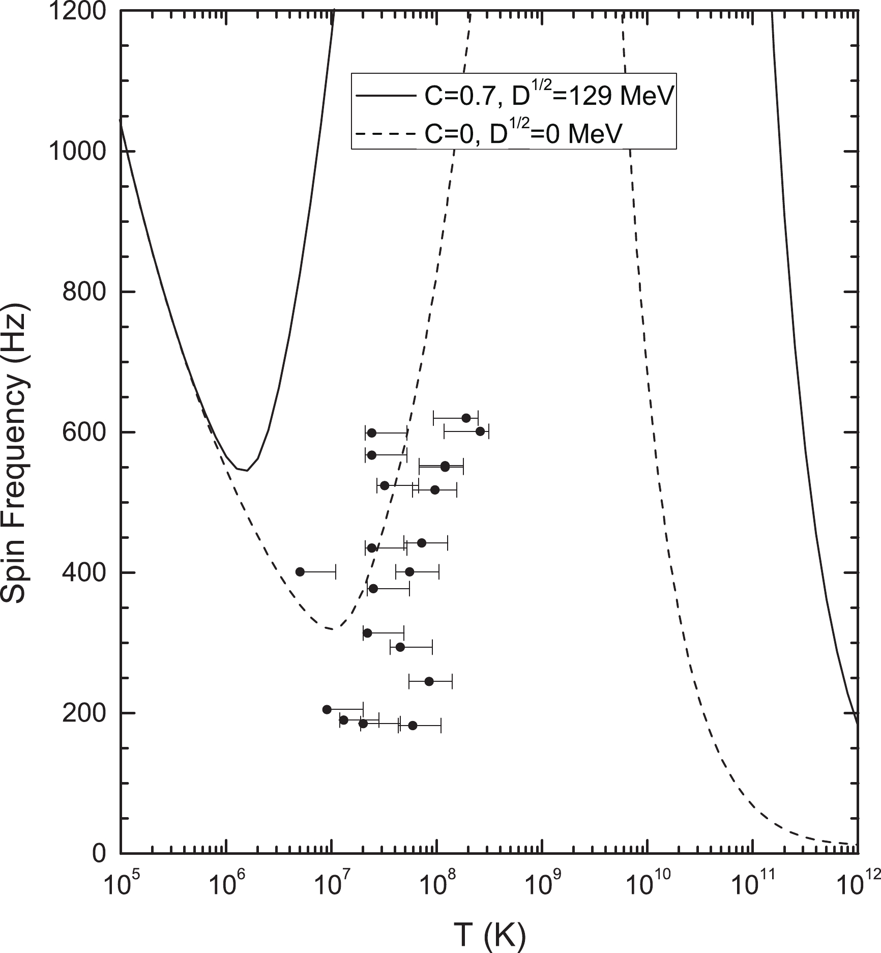
Figure 12.
$ R $ -mode (in)stability window for an assumed typical compact star with mass$ M=1.4\ \mathrm{M}_\odot $ and radius$ R = 10 $ km. Observational data on spin frequency and internal temperature of compact stars in LMXBs are also given.However, we mention that the typical strange star configuration assumed in Fig. 12 is not tolerated in our model, where according to Table 2, the radius of a strange star with
$M = 1.4\ {\rm M}_\odot$ is 14.38 km rather than 10 km. In Fig. 13, we thus present the$ r $ -mode instability window for realistic strange stars with$M = 1.4\ {\rm M}_\odot$ in our model. The solid line denotes the star with both quark confinement effects and perturbative interactions, whereas the dashed line represents the star merely with quark confinement. According to Fig. 13, although the absence of perturbative interactions locates one star (SAX J1808.4-3658) in the unstable region, it is obvious that with full interactions, our numerical results are still consistent well with the observational data.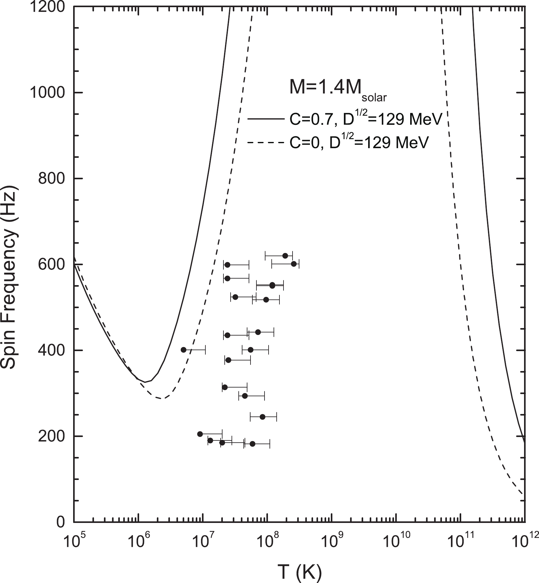
Figure 13.
$ R $ -mode (in)stability window for real stars in our model. The solid line denotes the star with both quark confinement effects and perturbative interactions, whereas the dashed line corresponds to the star merely with quark confinement.Nevertheless, we stress that the results obtained here are based on the calculations for bare strange quark stars. If compact stars, like hybrid stars [64], bear a nuclear matter envelope, surface rubbing effects can play an important role. Moreover, if strange stars are made of SQM in the 2SC phase [65] or CFL phase [21,54] of QCD [66], the shear viscosity due to electron-electron scattering plays a dominant role in dissipating radial oscillations, whereas the shear viscosity due to quark-quark scattering and bulk viscosity due to the nonleptonic weak interaction is less significant.
-
In this paper, we have investigated the bulk viscosity of SQM in the equivparticle model, which can be readily applied to those with other quark mass scalings. By taking constant masses for quarks, previous results in the bag model were reproduced. With a recently obtained quark mass scaling, we investigated the contributions of the quark confinement effects and perturbative interactions to the bulk viscosity of SQM and found that the contributions to the bulk viscosity from quark confinement effects significantly prevail over those from quark perturbative interactions. Due to the interactions between quarks, the dissipation rate in the equivparticle model is generally higher than that in the bag model, which therefore considerably enhances the magnitude of the bulk viscosity. This conclusion is in accordance with previous results [36,37,44]. However, we would like to point out that the model we employed here can yield strange quark stars with maximum mass larger than 2
${\rm M}_\odot$ , consistent with recent astrophysical observations [51,52].As for the application of the resulting bulk viscosity in astrophysics, we first studied the oscillation damping times of strange quark stars, from which we found that the damping times can be as short as a fraction of a millisecond for large relative amplitude oscillations. This could lead to rapid heating of strange stars after unstable activities such as starquakes, which may affect star evolutions and have meaningful implications for astronomical observation. Finally, we calculated the
$ r $ -mode instability windows for$1.4\ {\rm M}_\odot$ strange stars. Unlike those previously obtained in the bag model or modified bag model, the$ r $ -mode instability windows predicted by the new enlarged bulk viscosity are consistent with the observational data of stars in LMXBs.However, it should be pointed out that the conclusions obtained here are based on the assumption of bare strange stars. For compact stars with normal nuclear matter crust, strong magnetic field [34], 2SC or CFL SQM in the core, or superfluid neutron star cores [67], the current conclusion may be altered. Therefore, more effort should be devoted to these related issues. Additionally, the upper limit on spin frequency of pulsars in LMXBs has been updated from 716 Hz [68] to 1122 Hz [69], although the statistical significance of the latter is not very strong. Therefore, it is meaningful to examine the critical spin frequencies predicted by the model employed here with the parameters properly fixed. We leave this subject as one part of our future work.
Bulk viscosity for interacting strange quark matter and r-mode instability windows for strange stars
- Received Date: 2020-05-21
- Accepted Date: 2020-08-18
- Available Online: 2021-01-15
Abstract: We investigate the bulk viscosity of strange quark matter in the framework of the equivparticle model, where analytical formulae are obtained for certain temperature ranges, which can be readily applied to those with various quark mass scalings. In the case of adopting a quark mass scaling with both linear confinement and perturbative interactions, the obtained bulk viscosity increases by


 DownLoad: