


 Abstract
 HTML
HTML Reference
 Related
 PDF
PDF


-
Along the nuclear chart, there are a number of weakly bound states, as in the case of halo nuclei or isotopes close to the drip lines. These states are characterized by binding energies in the keV range rather than in the range of a few MeV, typical for nuclear binding. Such loosely (or weakly) bound states are thus located close to decay thresholds and the corresponding continuum of states. Under these circumstances, the coupling of such a bound state to the continuum can no longer be neglected; for reviews see, e.g., [1-3]. For conventional nuclear models, such as the shell model or the no-core-shell model, the coupling to the continuum based on, e.g., Berggren's representation [4, 5], which treats bound, resonant continuum states on the same footing, is well established, see, e.g., [6-8]. In addition, ab initio calculations for systems such as 4He+n+n and
$ A = 7 $ isotopes, which include continuum effects, have been performed [9-11].Nuclear lattice effective field theory (NLEFT) is a novel method for performing ab initio calculations in nuclear structure and reaction physics [12, 13]. The basic idea is to discretize space-time on a finite volume
$ L^3\times L_t $ , where$ L \, (L_t) $ is the spatial (temporal) size. Nucleons are placed on the lattice sites, and their interactions are given in terms of properly modified chiral potentials, consisting of pion exchanges and short-distance operators. Strong isospin-breaking effects and the long-ranged Coulomb potential are also included, leading to a number of intriguing results, such as the ab initio calculation of the Hoyle state in 12C [14] or the first microscopic calculation of low-energy$ \alpha -\alpha $ scattering [15]. What is missing in this framework is the coupling to the continuum. Clearly, on the lattice, we have only real-valued energies, so a direct application of the Berggren approach is not possible. However, as shown by Lüscher in his seminal work, the complex-valued scattering phase shift can be mapped onto the volume-dependence of the lattice energy levels [16, 17]. We seek a similar formalism to explicitly describe the continuum coupling.In this work, we use a simple model of a heavy core
$ A $ coupled to one or two nucleons$ N $ , as described in Sect. II. In Sect. III, we consider$ AN\to AN $ scattering and adjust the$ AN $ interaction such that a very weakly bound state emerges. Using the Hamiltonian formalism of Refs. [18-24], we calculate the energy levels of this system in a finite volume. The full$ ANN $ system is considered in Sect. IV, where we adjust the parameters so that there is no three-particle bound state, thereby allowing us to study the influence of the unbound third particle on the$ AN $ scattering matrix. We conclude with a summary and outlook in Sect. V. The Appendix contains a short discussion of the normalization of the scattering equation used. -
Consider a three-particle model (
$ ANN $ system), with the$ A $ particle having a mass that is about 10 times that of the$ N $ particle, which has mass$ m $ . The$ A $ particle thus mimics the nuclear core. To be specific, let us calculate$ AN\to AN $ scattering. For simplicity, we use a separable potential of the form$\begin{aligned}[b] V^{AN}_H(p, p') = &\dfrac{1}{\sqrt{2\omega_{A}(p)2\omega_{N}(p)}} g f(p,\Lambda)f(p',\Lambda)\\ & \times \dfrac{1}{\sqrt{2\omega_{A}(p)2\omega_{N}(p)}}\; , \end{aligned}$

(1) with the regulator function
$ f(p,\Lambda) = \dfrac{\Lambda^2}{p^2+\Lambda^2}\; , $

(2) where
$ \omega_i(q) = \sqrt{m_i^2+q^2} $ , and$ g $ is the coupling constant. The normalization is explained in the Appendix. In what follows, we set$ m_A = 10\, $ GeV, and$ m = \Lambda = 1\, $ GeV. We are interested in the case in which the$ AN $ system has a very weakly bound state$ B $ with binding energy in the keV range, so the coupling$ g $ is tuned accordingly.We can then construct the Hamiltonian in the finite volume and find its eigenvalues [19]. The Hamiltonian matrix is defined as follows:
$ \begin{aligned}[b] H = &H_0+H_I,\\ \left(H_{0}\right)_{ij} =& \delta_{ij}\left(\omega_A(k_i)+\omega_N(k_i)\right), \end{aligned} $

(3) $ \left(H_I\right)_{ij} = \dfrac{\sqrt{C_3(i)C_3(j)}}{4\pi} \left(\frac{2\pi}{L}\right)^3 V_H(E,k_i,k_j), $

(4) where
$ k_i = \sqrt{i}2\pi/L $ and$ C_3(i) $ represents the number of ways to sum the square of the three integers to equal$ i $ . Further, the factor$ (\sqrt{C_3(i)C_3(j)} \; )/(4\pi) (2\pi/L)^3 $ is due to the quantization in a finite box of size$ L $ , as explained in Refs. [18, 19].For the full
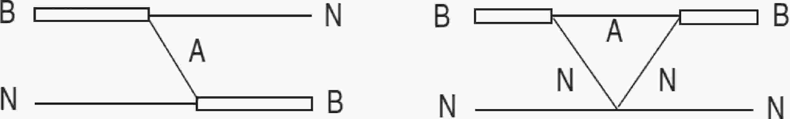
$ ANN $ system with a fixed total momentum, we have two free momenta. This leads to a Hamiltonian matrix with a huge dimension in the finite volume. For simplification, we thus consider the$ BN $ system instead of the$ ANN $ system; this means that we use a version of the dimer approximation, see, e.g., [25], reminiscent of the so-called Faddeev fixed center approximation, see, e.g., Refs. [26, 27]. We thus consider the scattering process$ BN\to BN $ .The left diagram in Fig. 1 shows the attractive interaction between
$ B $ and$ N $ since the$ AN $ system has a weak attractive interaction. To prepare this diagram, we need to obtain the coupling of the$ B\to AN $ process. Since$ B $ is a loosely bound state of$ AN $ , one can obtain the coupling from the amplitude of$ AN \to AN $ around the pole position of$ B $ as follows: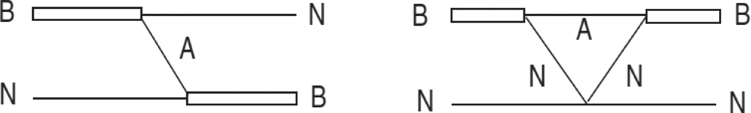
Figure 1. Effective diagrams for the
$ BN \to BN $ process.$\begin{aligned}[b] T^{AN}_H\Big(E\sim m_B, q = &q_0(E), q' = q_0(E) \Big) \\ =& \dfrac{1}{2m_{A}}\dfrac{1}{2m_{N}}4\pi \dfrac{\tilde{g}^2}{2m_B(E-m_B)}, \end{aligned}$

(5) where
$ q_0(E) $ is the on-shell momentum with energy$ E $ , and$ T^{AN}_H $ is obtained from Eq. (22) with the potential$ V^{AN}_H $ . The factor$ 1/(2m_{A}) \cdot 1/(2m_{N}) $ originates from the difference between$ V_H $ and$ V_L $ (see the Appendix). The momentum is on-shell, so it is close to the mass of the particle, and the factor$ 4\pi $ is from the angular integration since we only consider the s-wave. Further, the coupling$ \tilde{g} $ has dimension energy. Given this, the potential of$ BN \to BN $ from$ A $ -exchange takes the form$ \begin{aligned}[b] V^{BN1}_H(p, p') = & \dfrac{2\pi}{\sqrt{2\omega_B(p)2\omega_N(p)}} \\ &\times \int {\rm d} \cos\theta \dfrac{\tilde{g}^2} {(E_A^2)-(\vec{p}-\vec{p}\,')^2-m^2_A}\\ &\times\dfrac{1}{\sqrt{2\omega_B(p')2\omega_N(p')}}, \end{aligned} $

(6) $ E_A^2 = \frac{1}{2}\left((\omega_B(p)-\omega_N(p'))^2+\left(\omega_N(p)-\omega_B(p')\right)^2\right)\; . $

(7) Since our potential should be independent of the total energy, we take the average of the two processes
$ B\to AN $ and$ NA\to B $ . Next, we need to extract the s-wave contribution from this diagram, so we perform the angular integration between$ \vec{p} $ and$ \vec{p}\,' $ . Finally, the equation for the potential takes the form$ &V^{BN1}_H (p, p') = \dfrac{\tilde{g}^2}{\sqrt{2\omega_B(p)2\omega_N(p)2\omega_B(p')2\omega_N(p')}} \dfrac{\pi}{pp'} \ln\left(\dfrac{m_B^2+m_N^2-m_A^2-(\omega_B(p)\omega_N(p')+\omega_N(p)\omega_B(p'))+2pp'} {m_B^2+m_N^2-m_A^2-(\omega_B(p)\omega_N(p')+\omega_N(p)\omega_B(p'))-2pp'}\right). $

(8) Note that this potential should be negative because in Eq. (6), the propagator of the exchanged
$ A $ particle is negative.Now we consider the contribution from the right diagram in Fig. 1. This includes a triangle loop, and the main interaction is the
$ NN \to NN $ interaction. The$ NN \to NN $ interaction can be written as$\begin{aligned}[b] V^{NN}_H(p, p') =& \dfrac{1}{\sqrt{2\omega_{N}(p)2\omega_{N}(p)}} g_{NN} f(p,\Lambda)f(p',\Lambda)\\ &\times \dfrac{1}{\sqrt{2\omega_{A}(p)2\omega_{N}(p)}}\; , \end{aligned}$

(9) where the regulator function is chosen to be the same as that for the
$ AN $ interaction. In this model, we want to describe the situation in which the$ BN $ system cannot form a bound state. The coupling$ g_{NN} $ is the only parameter that allows this to be achieved.Next, we determine the potential based on the diagram on the right side of Fig. 1:
$\begin{aligned}[b] V^{BN2}_H(p, p') = & \dfrac{2\pi}{\sqrt{2\omega_{B}(p)2\omega_{N}(p)}} \int {\rm d}\cos\theta\, V^{BN2}_L(\vec{p},\vec{p}') \\ & \times \dfrac{1}{\sqrt{2\omega_{B}(p')2\omega_{N}(p')}}, \end{aligned}$

(10) where
$ \begin{aligned}[b] V^{BN2}_L(\vec{p},\vec{p}') = & \int {\rm d}^4q \; \tilde{g}^2 \dfrac{1}{q^2_0-\vec{q}^2-m^2_A} \dfrac{1}{(\omega_B(p)-q_0)^2-(\vec{p}-\vec{q})^2-m^2_N)} \dfrac{1}{(\omega_B(p')-q_0)^2-(\vec{p}'-\vec{q})^2-m^2_N} T^{L}_{NN} \\ \!=& \! \!\int\! {\rm d}^3\vec{q} \; \tilde{g}^2 \dfrac{1}{2\omega_A(q)} \dfrac{1}{(\omega_B(p)\!-\!\omega_A(q))^2\!-\!(\vec{p}-\vec{q})^2\!-\!m^2_N} \dfrac{1}{(\omega_B(p')-\omega_A(q))^2-(\vec{p}'-\vec{q})^2-m^2_N)} T^{NN}_{L}\; , \end{aligned} $

(11) where
$ T_{L}^{NN} $ is the amplitude of$ NN \to NN $ . In the calculation of$ T_{L}^{NN} $ , we make some further assumptions. First, we assume$ T_{L}^{NN} \sim V_{L}^{NN} $ , which should be acceptable since we are not interested in the detailed structure of the$ NN $ scattering amplitude. Moreover, we require this interaction in a boosted frame. Although the form of$ V_L $ is not Lorentz invariant, we can rewrite the potential in a special form and define all the inputs to the center-of-mass (CM) system. This means that we write$ V^{NN}_L $ as$ T^{NN}_{L} \sim V^{NN}_{L} = g_{NN} f(k^*,\Lambda)f(k'^*,\Lambda) , $

(12) $ k^{*\,2} = E_{NN}^2/4-m_N^2, $

(13) $ E_{NN}^2 = \left(\sqrt{(\vec{q}-\vec{p})^2+m_N^2}+\sqrt{\vec{p}^2+m_N^2}\;\right)^2-q^2, $

(14) $ k^{'*\,2} = E_{NN}^{'2}/4-m_N^2, $

(15) $ E_{NN}^{'2} = \left(\sqrt{(\vec{q}-\vec{p}^{\,'})^2+m_N^2}+\sqrt{\vec{p}^{\,'2}+m_N^2}\;\right)^2-q^2. $

(16) We then obtain
$ V_H^{BN2} $ as defined in Eqs. (10-16) as follows:$\begin{aligned}[b] V^{BN2}_H(p, p') = & \dfrac{4\pi^2}{\sqrt{2\omega_{B}(p)2\omega_{N}(p)2\omega_{B}(p')2\omega_{N}(p')}} \\ & \times \int q^2{\rm d}q \dfrac{\tilde{g}^2 g_{NN}}{2\omega_A(q)} H(p,q)H(p',q), \end{aligned}$

(17) where
$\begin{aligned}[b] H(p,q) = \int {\rm d}\cos\theta \dfrac{1}{m^2_B+m^2_A-m^2_N-2\omega_B(p)\omega_A(q)+2pq\cos\theta} \dfrac{4\Lambda^2}{\!\left(\sqrt{q^2+p^2-2pq\cos\theta+m_N^2}+\!\!\sqrt{p^2+m_N^2}\right)^2\!\!-\!\!q^2-4m_N^2+4\Lambda^2}\; , \end{aligned}$

(18) which can easily be evaluated numerically.
-
First, we need to fix the coupling constant
$ g $ . In the left panel of Fig. 2, we show the binding energy of the two-particle system as a function of the coupling$ g $ . The latter is chosen in a suitable range such that the binding is weak, and indeed, at$ g = -30.65 $ , there is no more bound state. In what follows, we choose$ g = -31.0 $ , for which one finds a loosely bound state at$ |E_B| = 11.15\, $ keV. In the right panel of Fig. 2, the corresponding scattering phase shift in the close-to-threshold region is shown; it exhibits the typical features of a weakly bound state close to the threshold.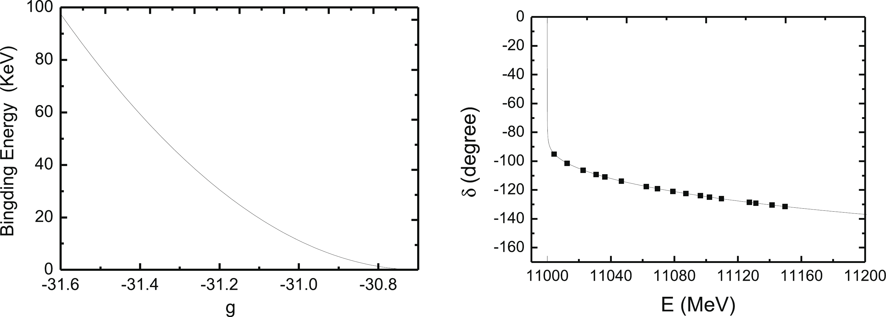
Figure 2. (left panel) Binding energy of the
$ AN $ system as a function of the coupling constant$ g $ . (right panel) Phase shift for$ AN\to AN $ scattering for$ g = -31.0 $ . The black points are calculated from the corresponding energy levels depicted in Fig. 3 using the Lüscher equation.The corresponding energy levels in the finite volume are shown in Fig. 3. The bound state level is clearly visible: its bending downwards for smaller lattice sizes is an expected finite volume effect. For sufficiently large
$ L $ , these finite volume effects are visibly absent.
Figure 3. Energy levels for the weakly bound
$ AN $ system in a finite volume$ L^3 $ . The meaning of the black squares at$ L = 10 $ fm is explained in text; see also Fig. 2.It is also instructive to compare our formalism with the Lüscher equation [16, 17]. For that, we select 17 energy levels at
$ L = 10 $ fm, and then, we use the following Lüscher equation to calculate the phase shifts from the corresponding energy levels:$ \delta(q_E) = \tan^{-1}\left(\frac{q_E L \sqrt{\pi}}{2 {\cal{Z}}(1; (\dfrac{q_EL}{2\pi})^2)} \right)+n\pi, $

(19) where
$ q_E $ is the on-shell momentum corresponding to the energy$ E $ :$ q_E = \frac{E}{2} \sqrt{\left(1-\left(\frac{m_N+m_A}{E}\right)^2\right)\left(1-\left(\frac{m_N-m_A}{E}\right)^2\right)}, $

(20) and
$ {\cal{Z}}(1;q^2) $ is the well known Zeta-function. After regularization, it can be calculated as follows:$\begin{aligned}[b] {\cal Z}(1; q^2) = &\sum\limits_{\vec{n}\in \mathbb{Z}^3}\dfrac{1}{\vec{n}^2-q^2} \\ =& -\dfrac{1}{q^2}-8.91363292+16.53231596 q^2 \\ &+ \sum\limits_{\vec{n}\in \mathbb{Z}^3}\dfrac{q^4}{\vec{n}^4\left(\vec{n}^2-q^2\right)}\; . \end{aligned}$

(21) We find that the phase shifts calculated in this way are all on the phase shift curve calculated directly from the scattering function, see Fig. 2. This shows that our calculation is consistent with the Lüscher equation.
-
Before showing the results, a few remarks are in order. We note that the atractive potential of
$ BN\to BN $ by$ A $ -exchange has a sizeable magnitude at the threshold because the propagator of the$ A $ -particle is very close to zero since$ B $ is a loosely bound state of$ AN $ . Similarly, the repulsive potential of$ BN\to BN $ generated by the triangle-loop also has a large value close to the threshold, since at that time, both nucleons can be close to their mass shell. We therefore consider various choices to adjust the coupling$ g_{NN} $ , cf. Eq. (9). One is for these two contributions to cancel exactly at the threshold (case 1), and another is for the total potential to be repulsive (case 2). In Fig. 4, we show the potential for various choices of the coupling$ g_{NN} $ .
Figure 4. (color online) Potentials in the
$ AN $ (black solid line) and the$ BN $ systems. In the latter case, two choices for the coupling$ g_{NN} $ are considered, as discussed in the text (blue dash-dotted and green dotted lines). The red dashed line shows the attractive$ BN $ potential from$ A $ -exchange.Case 1: With
$ g_{NN} = 48.34 $ , there is a repulsive$ BN\to BN $ interaction, but at the threshold, the potential is zero. Above the threshold, the potential increases rapidly and then drops with almost the same slope as that of the potential from the loop. From this potential, the corresponding finite volume spectrum can then be computed, as shown in the left panel of Fig. 5. It is surprising that there is still an energy level below the threshold of the$ BN $ system since there is pure repulsive potential. This is due to the strange structure of the potential at the threshold: at the threshold, the potential is exactly zero, and therefore, the first term of the full Hamiltonian matrix in the finite volume is simply the sum of the masses of$ B $ and$ N $ . In contrast, in the finite volume, the momentum is discrete. Therefore, the off-diagonal term in the Hamiltonian matrix provides an attractive potential whether the original potential is attractive or repulsive. Combing these two factors, the first energy level is lower than the threshold in the finite volume, especially for a small lattice size. The corresponding phase shift for$ BN\to BN $ is shown in the right panel of Fig. 5. It is almost the same as that for$ AN $ scattering, but we note that in the region very close to the threshold, the phase increases to about 10$ ^\circ $ , as shown in the inset of the right panel in Fig. 5. The steep fall-off of the phase can be traced back to the fast decrease in the potential, as shown by the green dotted curve in Fig. 4. We also compare our method to the Lüscher equation. The black points in the phase shift figure are calculated from the energy levels at$ L = 10 $ fm, which are shown as black points in the left panel of Fig. 5. With small fluctuations, all of the points are consistent with the curves of the phase shift, which are calculated directly from the scattering function. These fluctuations are discussed in the next case.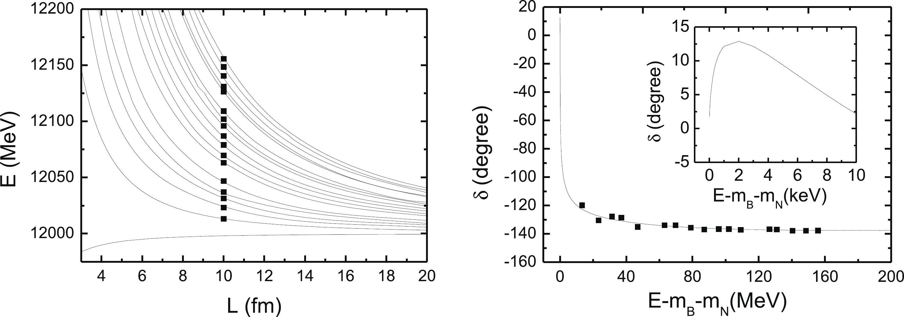
Figure 5. (left) Energy levels for the
$ BN $ system in a finite volume$ L^3 $ for$ g_{NN} = 48.34 $ . (right) Phase shift for$ BN\to BN $ . The inset shows the phase shift very close to the threshold. The black points in the left panel are the data at$ L = 10 $ fm. The black points in the right panel are calculated from the corresponding data in the left panel with$ L = 10 $ fm by using the Lüscher equation, as shown in Eq. (19).Case 2: With
$ g_{NN} = 96.68 $ , there is a repulsive interaction, and even at the threshold, it has a large value, although it still increases slightly with energy; see the blue dash-dotted line in Fig. 4. There is no bound state below the threshold in the finite volume spectrum, as shown in the left panel of Fig. 6. In this case, the phase shift exhibits similar behaviour to that in case 1 in the threshold region, but the magnitude is much smaller: the largest phase shift here is around$ 1^\circ $ . This corresponds to a potential barrier, so that the phase barely increases and very quickly starts to fall as fast as in case 1, as shown by the blue dash-dotted curve in Fig. 4. Analogous to case 1, we also check for consistency with the Lüscher equation. In the left panel in Fig. 6, the first four points are far away from the curve of the phase shift, which means that there is some inconsistency at low energy levels. In fact, our method differs systematically from the Lüscher equation in the difference between the summation and interaction of a regular function, as shown in the appendix of Ref. [19]. This difference is large when the regular function has a sharp structure, and it is proportional to$ \exp(-Lm) $ , where$ m $ is the scale corresponding to the variation in the potential close to the threshold. In our case, the potential contributes significantly to the regular function and varies quickly around the threshold. Therefore, the difference between summation and integration is very large in this case. However, in the$ A+N \to A+N $ case, the potential is much flatter, leading to perfect consistency between our method and the Lüscher equation, as shown in the left panel of Fig. 2. In other words, the fine structure at the threshold is absent in the finite volume when an insufficiently large volume is used. This can be resolved by increasing the lattice size, as shown in Fig. 6. The red circles corrsepsond to a larger volume of$ L = 17 $ fm and are consistent with the phase curve. Therefore, in principle, our method is consistent with the Lücher equation.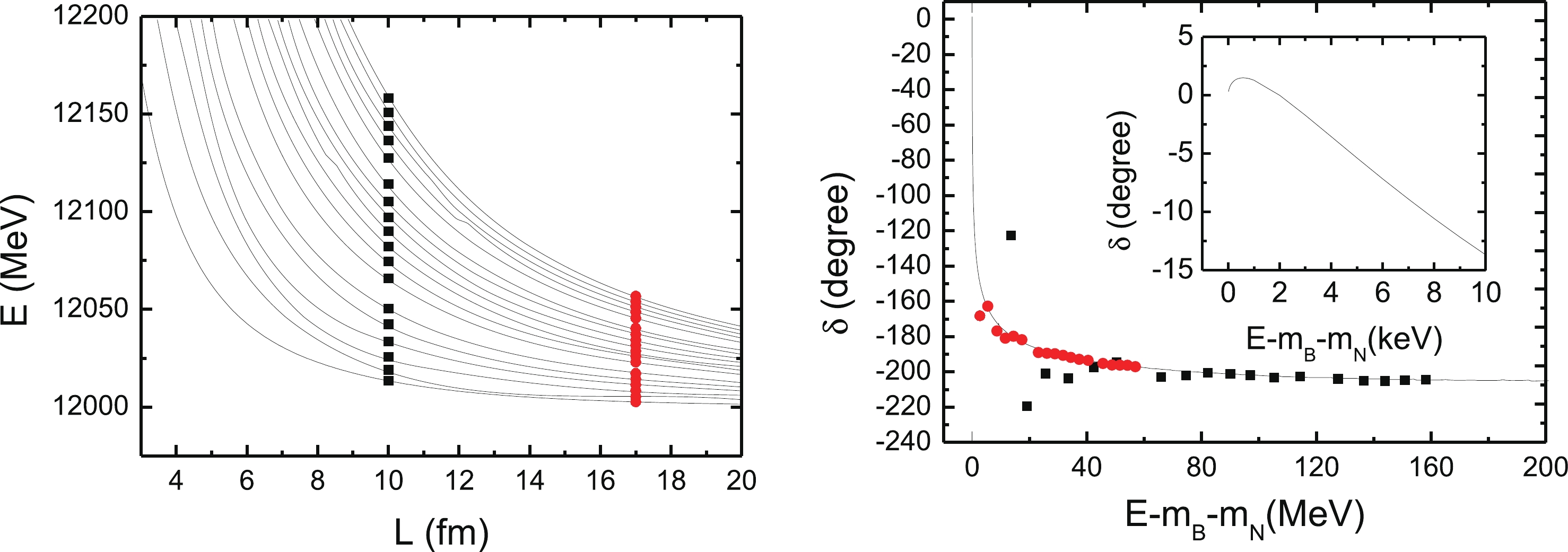
Figure 6. (color online) (left) Energy levels for the
$ BN $ system in a finite volume$ L^3 $ for$ g_{NN} = 96.68 $ . (right) Phase shift for$ BN\to BN $ . The inset shows the phase shift very close to the threshold. The black points and red circles in the left panel are the data at L = 10 fm and 17 fm, respectively. The black points and red circles in the right panel are calculated from the corresponding data in the left panel with L = 10 fm and 17 fm, respectively, using the Lüscher equation, as shown in Eq. (19).Based on these observations, we speculate that refined calculations will make it possible to find a compact formula for the influence of the continuum on a weakly bound state on the lattice.
-
In this letter, we have made the first step towards evaluating the influence of the continuum on weakly bound states. We have shown that there is a visible interplay between the weakly bound state
$ B $ in the two-particle system and the third particle, which leaves its traces in the lattice energy spectrum. To draw more definite conclusions, the model will require substantial refinement. As the first step, the full three-body$ ANN $ system should be investigated. Since the threholds of BN and ANN are very close, we expect that the inelastic effects due to the breakup reaction$ B + N \to A + N + N $ will affect the spectrum. Then, the interaction potentials need to be refined so that they more closely resemble the nuclear case. Higher partial waves also need to be included. Work along these lines is underway.We thank Dean Lee for a useful communication.
-
Here, we briefly discuss the normalization of our scattering T-mat-rix. This normalization is similar to the formalism used in Ref. [28]. Consider the s-wave of the process
$ AN\to AN $ , with the scattering function given by$ \begin{aligned}[b] T_H(E,|\vec{k}|, |\vec{k}'|) = &V_H(|\vec{k}|, |\vec{k}'|) + \int q^2 {\rm d}q V_H(|\vec{k}|,q)\\& \times \frac{1}{E-\omega_A(q)-\omega_N(q)+{\rm i}\epsilon} T_H(E, q, |\vec{k}'|)\; , \end{aligned} \tag{A1}$

(A1) where
$ \omega_i(q) = \sqrt{m_i^2+q^2} $ . Correspondingly, the Bethe-Salpter function, where$ k,k' $ are four-momenta, takes the form$ \begin{aligned}[b] T_L(P, k, k') = & V_L(P, k, k') + \int {\rm d}^4q V_L(P,k,q) \frac{1}{q^2-m_A^2+{\rm i}\epsilon} \\ &\times \dfrac{1}{(P-q)^2-m_N^2+{\rm i}\epsilon} T_L(P, q, k') . \end{aligned} \tag{A2}\!\!\!$

(A2) Actually, Eq. (A1) can be recognized as the three-dimensional reduction of Eq. (A2) by using
$ \int {\rm d}^4q \frac{1}{q^2-m_A^2+{\rm i}\epsilon} \frac{1}{(P-q)^2-m_N^2+{\rm i}\epsilon} \sim \int q^2 {\rm d}q \frac{1}{E-\omega_A(q)-\omega_N(q)+{\rm i}\epsilon}\frac{1}{2\omega_A(q)2\omega_N(q)}\; . \tag{A3}$

(A3) Therefore, we obtain the relationship between
$ V_H $ and$ V_L $ :$ V_H(E,|\vec{k}|,|\vec{k}'|) = \dfrac{2\pi}{\sqrt{2\omega_A(k)2\omega_N(k)}} \int {\rm d} \cos\theta V_L(P, k, k') \times \dfrac{1}{\sqrt{2\omega_A(k')2\omega_N(k')}}\; . \tag{A4}$

(A4) Note that we have been cavalier with some factors such as
$ (2\pi)^n $ since these are absorbed into the coupling in$ V_L $ . This equation is also the simple form of Eqs. (23,24) in Ref. [28].
Towards the continuum coupling in nuclear lattice effective field theory I: A three-particle model
- Received Date: 2020-07-21
- Available Online: 2020-12-01
Abstract: Weakly bound states often occur in nuclear physics. To precisely understand their properties, the coupling to the continuum should be worked out explicitly. As the first step, we use a simple nuclear model in the continuum and on a lattice to investigate the influence of a third particle on a loosely bound state of a particle and a heavy core. Our approach is consistent with the Lüscher formalism.


 DownLoad: