


 Abstract
 HTML
HTML Reference
 Related
 PDF
PDF


-
In recent decades, there have been rapid developments in the field of scattering amplitudes. For instance, complicated multi-loop amplitudes are being computed by new computational techniques [1-5], while new formalisms are being constructed that encode inspiring mathematical structures [6-14]. Among these advances, the study of the scattering amplitudes of gravity and gauge theories, as well as the intimate relationships between them, has attracted much attention. It is already well-known that there are non-trivial relationships between tree level color-ordered Yang-Mills amplitudes such as
$ U(1) $ -relations, Kleiss-Kuijf (KK) relations [15, 16], and Bern-Carrasco-Johansson (BCJ) relations [17, 18], which reduce the minimal number of independent color-ordered Yang-Mills amplitudes to$ (n-3)! $ . Regarding the gravity amplitude, the Kawai-Lewellen-Tye (KLT) relations [19], which originally state that a closed string amplitude is a combination of the products of two open string amplitudes, degenerate to similar relations between gravity and Yang-Mills amplitudes in the field theory limit. In addition, the BCJ double copy conjecture reveals another new way of constructing the gravity amplitude from Yang-Mills amplitudes based on the exciting idea of color-kinematic duality [17, 20, 21].In addition to these relations, the amplitudes of Einstein-Yang-Mills (EYM) theories where gravitons are allowed to interact with gauge bosons have also been investigated from many aspects [13, 14, 22, 23]. In particular, in [14], a generalized KLT relation is proposed from the study of Cachazo-He-Yuan (CHY) formalism [10-14], schematically formulated for the tree-level single-trace EYM amplitude① as
$\tag{1.1}\begin{aligned}[b] A^{{ \rm{EYM}}}_{r,s}(\alpha) =& \sum\limits_{\sigma,\tilde{\sigma}\in S_{n-3}} A^{{\rm{YM}}}_{n}(n-1,n,\sigma,1)\\&\times{\cal S}[\sigma|\tilde{\sigma}]A^{{\rm{YMs}}}_{r,s}(\alpha|1,\tilde{\sigma},n-1,n)\; ,\end{aligned} $

with
$ A^{{{\rm{YMs}}}} $ being the amplitudes of Yang-Mills-scalar theory and$ {\cal S} $ the momentum kernel, defined in [24-26]. Parallel to the study of monodromy relations in string theory, in [27], the authors present a new relation formulating the EYM amplitude with n gluons and one graviton as a linear combination of$ (n+1) $ -point Yang-Mills amplitudes in a compact expression. This result has been generalized to situations with more than one graviton [28, 29] and double color traces [28] in the framework of CHY formalism. Furthermore, in [30], by studying the constraints of gauge invariance, a compact recursive formula is presented for the expansion of EYM amplitudes with m gravitons in terms of the KK basis of color-ordered Yang-Mills amplitudes; the result has also been proven in the CHY formalism [31] and generalized to multi-trace amplitudes [32]. For the purpose of the current paper, we recall the expansion of EYM amplitudes to color-ordered Yang-Mills amplitudes in the KK basis, as in [30, 32],$\tag{1.2}\begin{aligned}[b] A^{{ \rm{EYM}}}_{n,m}(1,2,\ldots,n;{\bf{H}}) = \sum\limits_{\shuffle} \sum\limits_{{\bf{h}}|\tilde{h} = {\bf{H}}\backslash h_a} C_{h_a}({\bf{h}})\times A^{{ \rm{EYM}}}_{n+m-|\tilde{h}|,|\tilde{h}|} (1,\{2,\ldots,n-1\}\shuffle\{{\bf{h}},h_a\},n;\tilde{h})\; ,\end{aligned} $

where
$ {\bf{H}} = \{h_1,h_2,\cdots,h_m\} $ is a set of m gravitons, and$ \alpha\shuffle \beta $ stands for the shuffle permutations between two ordered sets$ \alpha,\beta $ , i.e., permutations of$ \alpha\cup\beta $ keeping the respective orderings of$ \alpha $ and$ \beta $ . In this expansion, legs$ 1 $ and n are always fixed in the first and last positions in the color-ordering. Hence, using the recursive formula, at the end, the EYM amplitude would be expanded to the basis of Yang-Mills amplitudes with legs$ 1 $ and n being fixed. The coefficient of each Yang-Mills amplitude is a linear combination of$ C_{h_a}({\bf{h}}) $ , which are polynomial functions of polarization vectors and momenta whose precise definition can be found in [30].While the expansion of the EYM amplitude in the KK basis of Yang-Mills amplitudes has been solved completely, as the KK basis is not the minimal basis of color-ordered Yang-Mills amplitudes, a question naturally arises: what would happen when expanding an EYM amplitude to the minimal basis, i.e., the BCJ basis of Yang-Mills amplitudes? At first glance, it seems that this question has already been solved by the generalized KLT relation (1.1). However, in (1.1), the momentum kernel
$ {\cal S}[\sigma|\tilde{\sigma}] $ and$ A_{R} $ are difficult to compute; we also need to sum over all$ S_{n-3} $ permutations. Hence, the generalized KLT relation does not work well with respect to practical computation. One could also start with expression (1.2) and reformulate the KK basis to the BCJ basis using the BCJ relations. However, computation of several examples is sufficient to suggest that the algebraic manipulations are rather complicated. The resulting expansion coefficients are rather cumbersome, without any hints of systematic and compact reorganization, because there are too many equivalent expressions. In [33], a new method is proposed by introducing differential operators into this problem. The differential operator was originally applied to the study of the relationships among the amplitudes of different theories [34], and later, a series of studies showed how to apply differential operators to the expansion of the EYM amplitude to the KK basis [33, 35, 36]. Then, differential operators were naturally applied to the expansion of the EYM amplitude into the BCJ basis, being limited to some simple cases where the EYM amplitudes contain one, two, or three gravitons. However, a systematic method for a generic EYM amplitude with n gluons and m gravitons is still needed.In this study, we attempt to fulfill this request by providing a systematic method for computing the expansion coefficients of the EYM amplitude with m gravitons in the BCJ basis. In addition to the use of differential operators, we also require the principle of gauge invariance. Because the Yang-Mills amplitudes of the BCJ basis are linearly independent, if we can write an EYM amplitude as a linear combination of Yang-Mills amplitudes of the BCJ basis, the gauge invariance of polarization tensors of gravitons would be transformed partially into the gauge invariance of expansion coefficients, which contain one half of the polarization vectors of the polarization tensors. Hence, the gauge invariance places strong constraints on the form of the expansion coefficients. In fact, the gauge invariance principle has already played an important role in the study of scattering amplitude. It is expected that the gauge invariance could completely determine the amplitudes of certain field theories [8, 37, 38], and further exploration can be found from various perspectives [30, 34, 39-42]. In particular, as demonstrated in [30], it is the constraints of gauge invariance that make a compact formula available for expansion of EYM amplitude in the KK basis. However, the potential applications of gauge invariance have still not been fully exploited. In this paper, we would like to propose a different understanding of gauge invariance. Similar to what we have performed for the symmetries in the amplitudes of
$ {\cal N} = 4 $ super-Yang-Mills theory, because the principle of gauge invariance is a strong constraint for gauge theory, we prefer to make it manifest at the level of scattering amplitudes.With the new understanding of gauge invariance, in this study, we will show how to expand the general EYM amplitude into the BCJ basis of Yang-Mills amplitudes systematically. This paper is organized as follows. In §2, we review some background. In §3, we introduce the gauge invariant vector space living in a general vector space consisting of polynomials of Lorentz contractions of momenta and polarization vectors. We compute the dimension of gauge invariant space, characterize the explicit form of vectors, and finally construct the gauge invariant basis. In §4, we define gauge invariant vectors and differential operators in quiver representation, which is the description of the mathematical structures of these vectors and operators. With the help of quivers, we implement a systematic algorithm to compute expansion coefficients. In §5, we illustrate our method using several explicit examples, e.g., the EYM amplitudes with up to four gravitons for the purpose of clarifying some subtleties. In §6, we conclude our discussion and point out some problems that remain to be solved in the future. Detailed proofs of some propositions as well as some explicit BCJ coefficients in the BCJ relations are presented in the appendices.
-
In this section, we review some background knowledge, which is useful in the subsequent discussion of expanding the EYM amplitude to the BCJ basis of Yang-Mills amplitudes. First, as reviewed in [33], an arbitrary color-ordered Yang-Mills amplitude can be expanded to the BCJ basis with three particles being fixed in certain positions related to the color-ordering, as follows:
$\tag{2.1} A_n (1,{\beta}_1,\cdots,{\beta}_r,2,{\alpha}_1,\cdots,{\alpha}_{n-r-3},n) = \sum\limits_{\{\xi\} \in \{{\beta}\} \shuffle_{\cal P} \{{\alpha}\}} {\cal C}_{\{{\alpha}\},\{{\beta}\};\{\xi\}} A_n(1,2,\{\xi\},n)\; . $

The expansion coefficients, i.e., the BCJ coefficients, were first conjectured in [17] and later proven in [18], using the expression
$\tag{2.2} {\cal C}_{\{{\alpha}\},\{{\beta}\};\{\xi\}} = \prod\limits_{k = 1}^r {{\cal F}_{{\beta}_k}(\{{\alpha}\},\{{\beta}\};\{\xi\}) \over {\cal K}_{1{\beta}_1...{\beta}_k}}\; .\; \; \; $

Notations in the above expression and explicit examples are presented in Appendix B.
Second, we review the differential operators that are originally introduced in [34]. An important differential operator is the insertion operator, defined as
$\tag{2.3} {\cal T}_{ik(i+1)}: = \partial_{k_i\cdot \epsilon_k}-\partial_{k_{i+1}\cdot \epsilon_k}\; .\; \; \; $

Physically, it represents changing a graviton k into a gluon and inserting it between i and
$ i+1 $ in the color ordering of gluons. If two gluons are not adjacent, for instance$ i, i+2 $ , we will have$\tag{2.4} {\cal T}_{ik(i+2)} = {\cal T}_{ik(i+1)}+{\cal T}_{(i+1)k(i+2)}\; ,\; \; \; $

and its physical meaning is also clear②. Another important operator is the gauge invariance differential operator, defined as
$ \tag{2.5} {\cal G}_{a}: = \sum\limits_{i\neq a} (k_a\cdot k_i) \frac{\partial}{\partial (\epsilon_a\cdot k_i)}+ \sum\limits_{j\neq a} (k_a\cdot \epsilon_j) \frac{\partial}{\partial (\epsilon_a\cdot \epsilon_j)}\; .\; \; \; $

It has a physical meaning of imposing gauge invariance, i.e., changing
$ \epsilon_a\to k_a $ . For an arbitrary polynomial of polarization vectors and momenta, if it vanishes under operator$ {\cal G}_a $ , we can conclude that it is gauge invariant for polarization vector$ \epsilon_a $ . Gauge invariance operators are commutative, i.e.,$ [{\cal G}_{a},{\cal G}_{b}] = 0 $ , so the result of a multiplication of sequential operators does not depend on the ordering, and we can denote a sequential gauge invariance operator as$\tag{2.6} {\cal G}_{i_1 i_2...i_s}: = {\cal G}_{i_1}{\cal G}_{i_2}\cdots {\cal G}_{i_s}\; \; \; ,\; \; \; i_1<i_2<\cdots <i_s\; .\; \; \; $

The insertion operator and gauge invariance operator satisfy the following commutative relation,
$\tag{2.7} [{\cal T}_{ijk},{\cal G}_{l}] = \delta_{li}{\cal T}_{ij}-\delta_{lk}{\cal T}_{jk}\; ,\; \; \; $

with
$ T_{ij}: = \partial_{(\epsilon_i\cdot \epsilon_j)} $ , and it is valid after application to any functions of polarization vectors and momenta ③.Finally, let us present a general discussion on the expansion of the EYM amplitude to the BCJ basis. For particles with spin, the corresponding Lorentz representations are constructed by polarizations, e.g., the polarization vector
$ \tilde{\epsilon}_i^{\; \mu} $ for gluons and polarization tensor$ \epsilon_{h_i}^{\mu\nu} $ for gravitons. When expanding the EYM amplitude to the BCJ basis, the polarization tensor of gravitons is factorized into two parts,$ \epsilon_{h_i}^{\mu\nu} = \tilde{\epsilon}_{h_i}^{\; \mu}\otimes \epsilon_{h_i}^{\nu} $ . The part$ \tilde{\epsilon}_{h_i}^{\; \mu} $ is inherent because of the polarization vector of gluons in the Yang-Mills basis, while the other part,$ \epsilon_{h_i}^{\nu} $ , is absorbed into the expansion coefficients. More explicitly, the expansion coefficients are rational functions of momenta$ k^\mu_\kappa, \kappa = 1,\cdots,n,h_1,\cdots,h_m $ and polarization vectors$ \epsilon^\mu_{h_\kappa}, \kappa = 1,\ldots,m $ . A crucial difference between expanding to the KK basis and BCJ basis is that the BCJ basis is truly an algebraic independent basis, and the corresponding expansion coefficients must be gauge invariant, i.e.,$\tag{2.8}{A^{{\rm{EYM}}}} = \sum {{c_{{\rm{gauge - inv}}}}} \times ({A^{{\rm{YM}}}}\;{\rm{in}}\;{\rm{BCJ}}\;{\rm{basis}})\;.$

This observation inspires us to consider another form of expansion:
$\tag{2.9}{A^{{\rm{EYM}}}} = \sum {({\rm{linear}}\;{\rm{sum}}\;{\rm{of}}\;{A^{{\rm{YM}}}})} \times {b_{{\rm{gauge - inv}}}}\;.$

In equation (2.8), independent Yang-Mills amplitudes are taken to be the expansion basis, and each coefficient as a function of momenta and polarization vectors
$ \epsilon_{h_\kappa} $ should satisfy the conditions of gauge invariance for all$ \epsilon_{h_\kappa} $ with$ \kappa = h_1, h_2,\ldots,h_m $ . In equation (2.9),$ b_{{\rm{gauge-inv}}} $ represents the expansion basis, and the expansion coefficients become a linear combination of$ A^{{\rm{YM}}} $ , with coefficients being rational functions of momenta. The latter form has already appeared in [33]; to distinguish the two different bases, we call$ b_{{\rm{gauge-inv}}} $ gauge invariant building blocks ④. -
As mentioned earlier, in the expansion of EYM amplitudes, the gauge invariant coefficients
$ c_{{ \rm{gauge-inv}}} $ as well as expansion basis$ b_{{\rm{gauge-inv}}} $ are crucial. They are polynomial functions of polarization vectors that vanish under conditions of gauge invariance. In this section, we would like to start from the most general vector space and localize a gauge invariant subspace of it. The expansion basis we are looking for is living in this exact subspace. -
Let us start from the most general polynomial
$ {\mathfrak{h}} $ , constructed by Lorentz contractions of n momenta$ k_1,k_2,\ldots,k_n $ and m polarizations$ \epsilon_1,\ldots,\epsilon_m $ with$ m\leqslant n $ . By Lorentz invariance and the multi-linearity of$ \epsilon_i $ , this polynomial must be formed schematically as$\tag{3.1} \begin{aligned}[b] {\mathfrak{h}}_{n,m}(k_1,\ldots,k_n,\epsilon_1,\ldots,\epsilon_m) =& \alpha_0(\epsilon\cdot k)^m+\alpha_1(\epsilon\cdot \epsilon)(\epsilon\cdot k)^{m-2}+\cdots\\&+\alpha_{\lfloor\frac{m}{2}\rfloor}(\epsilon\cdot \epsilon)^{\lfloor\frac{m}{2}\rfloor}(\epsilon\cdot k)^{m-\lfloor\frac{m}{2}\rfloor}\; ,\; \; \; \end{aligned}$

where for each monomial, the degree of
$ \epsilon $ is m, and each$ \epsilon_i, i = 1,\ldots,m $ appears once and only once, while the coefficients$ {\alpha} $ are rational functions of Mandelstam variables of momenta. If we take all monomials$ {\mathbb B}[V]: = \{ (\epsilon\cdot \epsilon)^j (\epsilon\cdot k)^{m-2j}\; ,\; 0\leqslant j\leqslant \lfloor\frac{m}{2}\rfloor \} $ as a generating set,⑤ then we can build up a vector space$ {\cal V}_{n,\{\epsilon_1,...,\epsilon_m\}} $ over the field of rational functions of Mandelstam variables, such that any polynomial$ {\mathfrak{h}}_{n,m} $ belongs to this vector space.To carve out the gauge invariant vector space from
$ {\cal V}_{n,\{\epsilon_1,...,\epsilon_m\}} $ , let us impose gauge invariant conditions on$ {\mathfrak{h}}_{n,m} $ . This can be achieved by applying differential operators$ {\cal G}_i $ to (3.1), i.e.,$ {\cal G}_i\; {\mathfrak{h}}_{n,m}: = {\mathfrak{h}}_{n,m-1}(\epsilon_i\rightarrow k_i)\; \; \; {\rm{for}}\;{\rm{each}}\; \; \; i = 1,...,m\; . $

This operator establishes a linear mapping between different vector spaces as
$\tag{3.2} {\cal V}_{n,\{\epsilon_1,...,\epsilon_m\}}\xrightarrow{{\cal G}_{t}} {\cal V}_{n,\{\epsilon_1,...,\epsilon_{t-1},\widehat \epsilon_t,\epsilon_{t+1},...,\epsilon_m\}}\; ,\; \; \; $

where in the resulting vector space, the polarization
$ \epsilon_t $ does appear and is replaced by$ k_t $ , denoted$ \widehat \epsilon_t $ . This linear map is surjective⑥ by noticing the reduction of$ {\mathbb B}[V] $ , i.e.,$\tag{3.3} {\rm{Im}}\; {\cal G}_t[{\cal V}_{n,\{\epsilon_1,...,\epsilon_m\}}] = {\cal V}_{n,\{\epsilon_1,...,\epsilon_{t-1},\widehat \epsilon_t,\epsilon_{t+1},...,\epsilon_m\}}\; .\; \; \; $

We can successively apply different gauge invariant operators
$ {{\cal G}}_i $ , with$ i = 1,\ldots,m $ , and establish a mapping chain of vector spaces. Because all$ {{\cal G}}_i $ are commutative, the result does not depend on the ordering of successive application, and we can denote the mapping chain as$\tag{3.4} {\cal V}_{n,m}\xrightarrow{{\cal G}_{i_1 i_2...i_s}} {\cal V}^{(i_1 i_2...i_s)}_{n,m-s}\; .\; \; \; $

The superscripts label the removed polarization vectors
$ \epsilon_i $ in the vector space. Note that different orderings of applying$ {\cal G}_i $ produce different mapping chains, which eventually lead to the same vector space, so (3.4) in fact represents a collection of mapping chains.The kernel of the linear map
$ {\cal G}_i:\; {\cal V}_{n,s}\to {\cal V}_{n,s-1}^{(i)} $ is defined by$\tag{3.5} {\rm{Ker}} \; {\cal G}_i[{\cal V}_{n,s}] = \{\; v\in {\cal V}_{n,s}\; |\; \; {\cal G}_i[{\cal V}_{n,s}] = 0\; \; \}\; .\; \; \; $

Physically, this means that the vectors of kernel are gauge invariant for the i-th particle. Using the fact that the linear map is surjective (4.3), by the fundamental theorem of linear mapping [43], we have
$\tag{3.6} \begin{aligned}[b] \dim {\cal V}_{n,s+1} =& \dim {\rm{Ker}}\; {\cal G}_i[{\cal V}_{n,s+1}]+\dim {\rm{Im}}\; {\cal G}_i[{\cal V}_{n,s+1}] \\=& \dim {\rm{Ker}}\; {\cal G}_i[{\cal V}_{n,s+1}]+\dim {\cal V}_{n,s}\; .\end{aligned} $

Then, the dimension of the kernel can be computed using the difference in the dimensions of vector space as
$\tag{3.7} \dim {\rm{Ker}}\; {\cal G}_i[{\cal V}_{n,s+1}] = \dim {\cal V}_{n,s+1}-\dim {\cal V}_{n,s}\; .\; \; \; $

When applying more than one
$ {\cal G}_i $ , this relation can be generalized to$\tag{3.8} \dim {\rm{Ker}}\; {\cal G}_{i_1 i_2.. i_t}[{\cal V}_{n,s}] = \dim {\cal V}_{n,s}-\dim {\cal V}_{n,s-t}\; .\; \; \; $

For example, let us consider the simplest case
$ s = 1 $ ,$ \tag{3.9} \dim {\rm{Ker}}\; {\cal G}_1[{\cal V}_{n,1}] = \dim {\cal V}_{n,1}-\dim {\cal V}_{n,0}\; .\; \; \; $

Vector space
$ {\cal V}_{n,0} $ is the field of rational functions of Mandelstam variables, so the basis is simply$ 1 $ , and$ \dim {\cal V}_{n,0} = 1 $ . For a vector space with only one polarization, the kernel$ {\rm{Ker}}\; {\cal G}_1[{\cal V}_{n,1}] $ consists of all vectors vanishing under the gauge invariant operator. This is the gauge invariant vector sub-space$ {\cal W}_{n,1} $ in a vector space$ {\cal V}_{n,1} $ . Thus, we have$ \tag{3.10} \dim {\cal W}_{n,1}: = \dim {\rm{Ker}}\; {\cal G}_1[{\cal V}_{n,1}] = \dim {\cal V}_{n,1}-1\; .\; \; \; $

For a general vector space
$ {\cal V}_{n,m} $ with m polarizations, we can define the gauge invariant vector sub-space as the intersection of kernels of all possible linear maps$ {\cal G}_i $ as$\tag{3.11}\begin{aligned}[b] {\cal W}_{n,m}: =& \bigcap\limits_{i = 1}^m {\rm{Ker}}\; {\cal G}_i[{\cal V}_{n,m}] \\ =& \{\; v\in {\cal V}_{n,m}\; |\; \; {\cal G}_i(v) = 0\; \; \forall i = 1,2,\ldots,m\; \}\; .\end{aligned} $

This means that a vector in
$ {\cal W}_{n,m} $ would vanish under any linear map$ {\cal G}_i $ . This is exactly the sub-space where all gauge invariant coefficients$ c_{{ \rm{gauge-inv}}} $ of (2.8) and the expansion basis$ b_{{\rm{gauge-inv}}} $ of (2.9) live.Let us attempt to compute the dimension of
$ {\cal W}_{n,m} $ and start with the case$ m = 2 $ . Generally, for any two linear spaces$ U_1, U_2 $ , we have the following relation for the dimension⑦,$\tag{3.12} \dim U_1+ \dim U_2 = \dim (U_1+U_2)-\dim (U_1\bigcap U_2)\; .\; \; \; $

Applying this relation to the vector spaces of kernels, i.e.,
$ U_i = {\rm{Ker}}\; {\cal G}_i[{\cal V}_{n,m}] $ , we get$\tag{3.13} \begin{aligned}[b] \dim {\cal W}_{n,2}: = & \dim \left({\rm{Ker}}\; {\cal G}_1\cap {\rm{Ker}}\; {\cal G}_2 \right) = \dim {\rm{Ker}}\; {\cal G}_1+\dim {\rm{Ker}}\; {\cal G}_2 \\ -& \dim \left({\rm{Ker}}\; {\cal G}_1+{\rm{Ker}}\; {\cal G}_2 \right) . \end{aligned} $

The first two terms in the RHS can be computed using (3.7), and to compute the third term, we need to use the following proposition ⑧,
PROPOSITION 1: any two kernels of linear maps
$ {\cal G}_{i} $ satisfy the splitting formula,$ \tag{3.14} {\rm{Ker}}\; {\cal G}_1+{\rm{Ker}}\; {\cal G}_2 = {\rm{Ker}}\; {\cal G}_{12} \; ,\; \; \; $

and its generalization,
PROPOSITION 1 EXTENDED: the kernels of linear maps
$ {\cal G}_{i} $ satisfy the generalized splitting formula,$\tag{3.15} {\rm{Ker}}\; {\cal G}_1+{\rm{Ker}}\; {\cal G}_2+\cdots +{\rm{Ker}}\; {\cal G}_m = {\rm{Ker}}\; {\cal G}_{12...m}\; .\; \; \; $

Together with (3.8), we can rewrite (3.13) as
$ \tag{3.16}\begin{aligned}[b]\dim {\cal W}_{n,2} = &2 (\dim {\cal V}_{n,2}-\dim {\cal V}_{n,1})-(\dim {\cal V}_{n,2}-\dim {\cal V}_{n,0}) \\=& \dim {\cal V}_{n,2}-2\dim {\cal V}_{n,1}+\dim {\cal V}_{n,0}\; .\end{aligned} $

Recursively using (3.12), we need to generalize the above result to arbitrary m. For simplicity, let us denote
$ U_i: = {\rm{Ker}}\; {\cal G}_i $ , and when$ m = 3 $ , we have$\tag{3.17} \begin{aligned}[b] \dim (U_1+U_2+U_3)& = \dim (U_1+U_2)+\dim U_3\\&-\dim ((U_1+U_2)\cap U_3) = \dim U_1\\ &+\dim U_2+\dim U_3-\dim (U_1\cap U_2)\\ &-\dim ((U_1+U_2)\cap U_3)\; .\\[-15pt] \end{aligned} $

In the second line, the first three terms have already been computed, while to compute the fourth term, we need to use the following proposition. ⑨
PROPOSITION 2: three kernels of linear maps
$ {\cal G}_{i} $ satisfy the distribution formula,$\tag{3.18} \begin{aligned}[b] ({\rm{Ker}}\; {\cal G}_1+{\rm{Ker}}\; {\cal G}_2)\cap {\rm{Ker}}\; {\cal G}_3 =& {\rm{Ker}}\; {\cal G}_1\cap {\rm{Ker}}\; {\cal G}_3\\&+{\rm{Ker}}\; {\cal G}_2\cap {\rm{Ker}}\; {\cal G}_3\; , \end{aligned} $

and its generalization,
PROPOSITION 2 EXTENDED: the kernels of linear maps
$ {\cal G}_{i} $ satisfy the generalized distribution formula,$\tag{3.19} \left(\sum\limits_{i = 1}^{m-1}{\rm{Ker}}\; {\cal G}_i\right)\cap {\rm{Ker}}\; {\cal G}_m = \sum\limits_{i = 1}^{m-1}{\rm{Ker}}\; {\cal G}_i\cap{\rm{Ker}}\; {\cal G}_m\; .\; \; \; $

Together with (3.12), we can rewrite (3.17) as
$ \tag{3.20}\begin{aligned}[b] &\dim ({\rm{Ker}}\; {\cal G}_1+{\rm{Ker}}\; {\cal G}_2+{\rm{Ker}}\; {\cal G}_3) = \dim {\rm{Ker}}\; {\cal G}_1+\dim {\rm{Ker}}\; {\cal G}_2\\&\quad\!+\!\dim {\rm{Ker}}\; {\cal G}_3\!-\!\dim ({\rm{Ker}}\, {\cal G}_1\!\cap\! {\rm{Ker}}\, {\cal G}_2) \! -\!\dim ({\rm{Ker}}\, {\cal G}_1\cap {\rm{Ker}}\, {\cal G}_3)\\&\quad\!-\!\dim ({\rm{Ker}}\; {\cal G}_2\cap {\rm{Ker}}\; {\cal G}_3)+\dim ({\rm{Ker}}\; {\cal G}_1\cap {\rm{Ker}}\; {\cal G}_2\cap {\rm{Ker}}\; {\cal G}_3) . \end{aligned} $

In equation (3.20), to compute the dimension
$ \dim {\cal W}_{n,3}: = \dim ({\rm{Ker}}\; {\cal G}_1\cap {\rm{Ker}}\; {\cal G}_2\cap {\rm{Ker}}\; {\cal G}_3) $ , we need the result of$ \dim ({\rm{Ker}}\; {\cal G}_1+{\rm{Ker}}\; {\cal G}_2+{\rm{Ker}}\; {\cal G}_3) $ , which by proposition 1 extended (3.15) is equal to$ \dim {\rm{Ker}}\; {\cal G}_{123} $ . Using (3.8), we get$\tag{3.21} \begin{aligned}[b]& \dim {\rm{Ker}}\; {\cal G}_i = {\cal V}_{n,3}-{\cal V}_{n,2},\quad \dim {\rm{Ker}}\; {\cal G}_{ij} = {\cal V}_{n,3}-{\cal V}_{n,1}\, ,\\& \dim {\rm{Ker}}\; {\cal G}_{ijk} = {\cal V}_{n,3}-{\cal V}_{n,0}\; .\\[-16pt]\end{aligned} $

Then,
$\tag{3.22} \dim {\cal W}_{n,3} = \dim {\cal V}_{n,3}-3\dim {\cal V}_{n,2}+3\dim {\cal V}_{n,1}-\dim {\cal V}_{n,0}\; .\; \; \; $

Notice that the numerical factors
$ 1,3,3,1 $ are nothing but$ \binom{3}{i} $ for$ i = 0,1,2,3 $ .Let us proceed further to arbitrary m. With proposition 1 extended and proposition 2 extended, equations (3.13) and (3.20) are exactly the same as the principle of inclusion-exclusion. By the well-known principle of inclusion-exclusion, we obtain
$\tag{3.23} \dim \left(\sum\limits_{i = 1}^{m} {\rm{Ker}}\; {\cal G}_i\right) = \sum\limits_{s = 1}^{m}(-)^{s-1} \sum\limits_{{\rm{all}}\; s-{\rm{subsets}}} \dim \left(\bigcap\limits_{j = 1}^{s} {\rm{Ker}}\; {\cal G}_{i_j}\right)\; ,\; \; \; $

where the second summation is over all subsets with s indices. It is also well-known that starting from the principle of inclusion-exclusion, we can arrive at
$\tag{3.24} \dim \left(\bigcap\limits_{i = 1}^{m} {\rm{Ker}}\; {\cal G}_i\right) = \sum\limits_{s = 1}^{m}(-)^{s-1}\sum\limits_{{\rm{all}}\; s-{\rm{subsets}}} \dim \left(\sum\limits_{j = 1}^{s} {\rm{Ker}}\; {\cal G}_{i_j}\right)\; .\; \; \; $

By proposition 1 extended, we can write
$\tag{3.25} \dim \left(\sum\limits_{j = 1}^{s} {\rm{Ker}}\; {\cal G}_{i_j}\right) = \dim {\rm{Ker}}\; {\cal G}_{i_1i_2\cdots i_s} = \dim {\cal V}_{n,m}-\dim {\cal V}_{n,m-s}\; .\; \; \; $

Substituting (3.25) back into (3.24), we get
$ \tag{3.26}\begin{aligned}[b] \dim {\cal W}_{n,m}: = \dim \ \left(\bigcap\limits_{i = 1}^m {\rm{Ker}}\ {\cal G}_i\right) =& \sum\limits_{s = 1}^m \sum\limits_{i_1<\cdots<i_s}(-1)^{s-1} ( \dim \ {\cal V}_{n,m}-\dim \ {\cal V}_{n,m-s}^{(i_1\cdots i_s)}) \\ = & \sum\limits_{s = 1}^m (-1)^{s-1}\binom{m}{s}\dim \ {\cal V}_{n,m}+\sum\limits_{s = 1}^m (-1)^{s}\binom{m}{s}\dim \ {\cal V}_{n,m-s} \\ = & \sum\limits_{s = 0}^m (-1)^{s}\binom{m}{s}\dim \ {\cal V}_{n,m-s}\; ,\; \; \; \end{aligned} $

where the dimension of vector space
$ {\cal V}_{n,m} $ can be computed via⑩$ \tag{3.27} \dim {\cal V}_{n,m} = \sum\limits_{i = 0}^{\lfloor \frac{m}{2}\rfloor} \binom{m}{2i} \frac{(2i)!}{2^i\; (i!)}(n-2)^{m-2i}\; .\; \; \; $

Hence, the dimension of arbitrary gauge invariant vector space
$ {\cal W}_{n,m} $ can be computed using equations (3.26) and (3.27).Let us present a few examples demonstrating the computation of dimensions. For the special case
$ m = n $ ,$ \dim {\cal W}_{n,n} $ values for the first few n values are listed as follows.n 4 5 6 7 8 9 10 $\dim {\cal W}_{n,n}$ 

10 142 2364 45028 969980 23372550 623805784 In [37], the same result has been provided up to
$ n = 7 $ ⑪. Compared with that result, our calculation shows more efficiency than that shown by solving linear equations of gauge invariance directly. Furthermore, several examples of$ \dim {\cal W}_{n,m} $ and$ \dim {\cal W}_{n+m,m} $ with arbitrary n but definite values of m are listed below.m 1 2 3 4 $\dim {\cal W}_{n,m}$ 

$n-3$ 

$(n-3)^2+1$ 

$(n-3)^3+3(n-3)$ 

$(n-3)^4+6(n-3)^2+3$ 

$\dim {\cal W}_{n+m,m}$ 

$n-2$ 

$(n-1)^2+1$ 

$n^3+3n$ 

$(n+1)^4+6(n+1)^2+3$ 

-
The dimension of gauge invariant vector space characterizes the minimal number of vectors required to expand an arbitrary vector, while the explicit form of the vector is not constrained. From the working experiences of EYM amplitude expansion with one, two, and three gravitons [33], we get the insight that the coefficients appearing therein could be recast in a manifestly gauge invariant form as linear combinations of multiplication of fundamental f-terms. Here, the fundamental f-terms stand for two types of Lorentz contractions of field strength
$ f_i^{\mu\nu} = k_i^{\mu}\epsilon_i^{\nu}-\epsilon_i^{\mu}k_i^{\nu} $ and external momenta, with at most two$ f_i $ ,$\tag{3.28} {\rm{Fundamental}}\;f{\rm{ - terms:}}\; \; \; \; \; \; \; \; \; k_i\cdot f_a \cdot k_j\; \; \; {\rm{and}}\; \; \; k_i\cdot f_a\cdot f_b\cdot k_j\; .\; \; \; $

This observation can be generalized beyond
$ m = 3 $ and can be stated as follows. For any vector in gauge invariant vector space$ {\cal W}_{n,m} $ with$ m<n $ ⑫,every vector in
$ {\cal W}_{n,m} $ can be recast in a manifestly gauge invariant form, as a linear combination of the multiplications of fundamental f-terms with the total number of field strength f in every monomial being m.We shall prove this statement by induction. The cases with
$ m = 1,2,3 $ have already been shown to be true in [33]. Following the idea of induction, we assume that this statement is true for all$ s<m $ and prove that it must be true for m.A polynomial
$ {\mathfrak{h}}_{n,m}\in {\cal W}_{n,m} $ with m polarizations$ \epsilon_1,\epsilon_2,\ldots, \epsilon_m $ can be generally written as$\tag{3.29} {\mathfrak{h}}_{n,m} = \sum\limits_{i = 2}^{m}(\epsilon_1\cdot \epsilon_i) T_{1i}+\sum\limits_{i = 2}^{m}(\epsilon_1\cdot k_i)(\epsilon_i\cdot T'_{1i})+\sum\limits_{i = m+1}^{n-1}(\epsilon_1\cdot k_i)T''_{1i}\; ,\; \; \; $

where momentum conservation has been applied to eliminate
$ \epsilon_1\cdot k_n $ , so that all$ (\epsilon_1\cdot \epsilon_i), (\epsilon_1\cdot k_i) $ appearing in$ {\mathfrak{h}}_{n,m} $ are linearly independent. Polynomials$ T_{1i}\in {\cal V}_{n,m-2} $ and$ \epsilon_i\cdot T'_{1i}\; ,\; T''_{1i}\in {\cal V}_{n,m-1} $ . Because$ {\mathfrak{h}}_{n,m}\in {\cal W}_{n,m} $ , by definition, we have$ \tag{3.30} {\cal G}_a \; {\mathfrak{h}}_{n,m} = 0\; \; \; ,\; \; \; \forall(1\leqslant a\leqslant m)\; .\; \; \; $

From the operator equation (2.7), we explicitly have
$ [{\cal T}_{a1n},{\cal G}_a] = {\cal T}_{a1} $ with$ a = 2,\cdots,m $ . Applying this to$ {\mathfrak{h}}_{n,m} $ generates a set of equations as follows:$\tag{3.31}\begin{aligned}[b] [{\cal T}_{a1n},{\cal G}_a]{\mathfrak{h}}_{n,m} =& {\cal T}_{a1}{\mathfrak{h}}_{n,m} \; \to\; -{\cal G}_a(\partial_{\epsilon_1\cdot k_a}-\partial_{\epsilon_1\cdot k_n}){\mathfrak{h}}_{n,m} \\=& \partial_{\epsilon_1\cdot \epsilon_a}{\mathfrak{h}}_{n,m} \; \to\; -(k_a\cdot T'_{1a}) = T_{1a}\; ,\end{aligned}$

where we have considered the fact that
$ {\mathfrak{h}}_{n,m} $ does not contain$ (\epsilon_1\cdot k_n) $ . With the above result, we can rewrite$ {\mathfrak{h}}_{n,m} $ as$\tag{3.32} {\mathfrak{h}}_{n,m} =\sum\limits_{i_1 = 2}^{m}(\epsilon_1\cdot f_{i_1} \cdot T'_{1i_1}) +\sum\limits_{i_1 = m+1}^{n-1}(\epsilon_1\cdot k_{i_1})T''_{1i_1}\; .\; \; \; $

We also need to consider the gauge invariance of
$ {\mathfrak{h}}_{n,m} $ with respect to the polarization vector$ \epsilon_1 $ ,$\tag{3.33} \begin{align} {\mathfrak{h}}_{n,m}(\epsilon_1\rightarrow k_1) = \sum\limits_{i_1 = 2}^{m}(k_1\cdot f_{i_1} \cdot T'_{1i_1}) +\sum\limits_{i_1 = m+1}^{n-1}(k_1\cdot k_{i_1})T''_{1i_1} = 0\; .\; \; \; \end{align} $

Then, we get
$\tag{3.34} \begin{align} T''_{1(n-1)} = -\sum\limits_{i_1 = 2}^{m}\frac{(k_1\cdot f_{i_1} \cdot T'_{1i_1})}{(k_1\cdot k_{n-1})} -\sum\limits_{i_1 = m+1}^{n-2} \frac{(k_1\cdot k_{i_1})}{(k_1\cdot k_{n-1})} T''_{1i_1}\; .\; \; \; \end{align} $

After substituting the above results back into
$ {\mathfrak{h}}_{n,m} $ , we get$\tag{3.35} \begin{align} {\mathfrak{h}}_{n,m} = & \sum\limits_{i_1 = 2}^{m}\frac{(k_{n-1}\cdot f_1\cdot f_{i_1} \cdot T'_{1i_1})}{(k_1\cdot k_{n-1})} +\sum\limits_{i_1 = m+1}^{n-2} \frac{(k_{n-1}\cdot f_1\cdot k_{i_1})}{(k_1\cdot k_{n-1})} T''_{1i_1}\; .\; \; \; \end{align} $

Therefore,
$ {\mathfrak{h}}_{n,m} $ is already manifestly gauge invariant for polarization vector$ \epsilon_1 $ . In fact, we can also choose to eliminate other coefficients in (3.34) and introduce different poles in the denominator of$ {\mathfrak{h}}_{n,m} $ .We can also generate another set of equations by considering the operator relations
$ [{\cal T}_{i1n},{\cal G}_a] \!= \!0 $ with$ i \!=\! m\!+\!1,$ $\cdots, n-2 $ and$ a = 2,\cdots,m $ . Applying them to$ {\mathfrak{h}}_{n,m} $ produces$\tag{3.36} \begin{align} [{\cal T}_{i1n},{\cal G}_a]{\mathfrak{h}}_{n,m} = 0 \to -{\cal G}_a(\partial_{\epsilon_1\cdot k_i}-\partial_{\epsilon_1\cdot k_n}){\mathfrak{h}}_{n,m} = 0\to {\cal G}_aT''_{1i} = 0\; ,\; \; \; \end{align} $

which means that
$ T''_{1i_1} $ is gauge invariant for$ \epsilon_{2},\epsilon_3,\cdots,\epsilon_m $ . By assumption of induction,$ T''_{1i_1} $ can be written as a linear combination of the multiplication of fundamental f-terms. Because$ {\mathfrak{h}}_{n,m} $ and$ T''_{1i_1} $ are gauge invariant for$ \epsilon_a $ with$ a = 2,\cdots,m $ , and$ (k_{n-1}f_1f_{i_1}T'_{1i_1}) $ are linearly independent,$ T'_{1i_1} $ is also gauge invariant for all of its own polarization vectors. Again, by assumption of induction, any$ (A f_{i_1} T'_{1i_1}) $ can also be written in a manifest gauge invariant form where only f appears. Thus, as a linear function of$ (k_{n-1}\cdot f_1\cdot f_{i_1} \cdot T'_{1i_1}) $ and$ T''_{1i_1} $ , the polynomial$ {\mathfrak{h}}_{n,m} $ can also be written in a manifest gauge invariant form, and we have proven the first part of our statement.To complete our proof, we need to apply the above procedure to
$ (\epsilon_{i_1}\cdot T'_{1i_1}) $ in (3.29) and rewrite it as$\tag{3.37} \begin{aligned}[b] (\epsilon_{i_1}\cdot T'_{1i_1}) =& \sum\limits_{i_2 = 2,i_2\ne i_1}^{m}(\epsilon_{i_1}\cdot \epsilon_{i_2})T_{1i_1i_2} +\sum\limits_{i_2 = 2,i_2\ne i_1}^{m} (\epsilon_{i_1}\cdot k_{i_2})(\epsilon_{i_2}\cdot T'_{1i_1i_2}) \\& +\sum\limits_{i_2 = m+1}^{n-1,1}(\epsilon_{i_1}\cdot k_{i_2})T''_{1i_1i_2}\; ,\; \; \; \end{aligned} $

where in the last summation,
$ i_2 $ can be equal to$ 1 $ . Let us again apply the operator equations$ [{\cal T}_{ai_1 n},{\cal G}_a] = {\cal T}_{ai_1} $ , with$ a = 2,\cdots,m $ and$ a\ne i_1 $ , which generates a set of equations,$\tag{3.38} \begin{align} (\epsilon_{i_1}\cdot T'_{1i_1}) = &\sum\limits_{i_2 = 2,i_2\ne i_1}^{m} (\epsilon_{i_1}\cdot f_{i_2}\cdot T'_{1i_1i_2}) +\sum\limits_{i_2 = m+1}^{n-1,1}(\epsilon_{i_1}\cdot k_{i_2})T''_{1i_1i_2}\; .\; \; \; \end{align} $

Therefore,
$ {\mathfrak{h}}_{n,m} $ becomes$\tag{3.39} \begin{aligned}[b] {\mathfrak{h}}_{n,m} =& \sum\limits_{i_1 = 2}^{m}\sum\limits_{i_2 = 2,i_2\ne i_1}^{m} \frac{(k_{n-1}f_1f_{i_1}f_{i_2}T'_{1i_1i_2})}{(k_1k_{n-1})} \\&+\sum\limits_{i_1 = 2}^{m}\sum\limits_{i_2 = m+1}^{n-1,1} \frac{(k_{n-1}f_1 f_{i_1} k_{i_2})}{(k_1k_{n-1})} T''_{1i_1i_2} +\sum\limits_{i_1 = m+1}^{n-2} \frac{(k_{n-1}f_1 k_{i_1})}{(k_1k_{n-1})}T''_{1i_1}\; .\; \; \; \end{aligned} $

Then, we apply
$ [{\cal T}_{ji_1n},{\cal G}_a] = 0 $ with$ j = m+1,m+2,\cdots, $ $n-1,1 $ and$ a = 2,\cdots,i_1-1,i_1+1,\cdots,m $ to$ (\epsilon_{i_1}\cdot T'_{1i_1}) $ , which leads to$ {\cal G}_a T''_{1i_1j} = 0 $ . It says that$ T''_{1i_1i_2} $ is gauge invariant for its own polarization vectors and can be written as a linear combination of the multiplication of fundamental f-terms. For the same reason as before, we conclude that$ T'_{1i_1i_2} $ is also gauge invariant for its own polarization vectors. Continuously applying the same procedure to$ T' $ until the last polarization vector, we arrive at$ \tag{3.40} {\mathfrak{h}}_{n,m} = \sum\limits_{s = 2}^{m}\widetilde{{\mathfrak{h}}}_{n,s}+\sum\limits_{i = m+1}^{n-2}\frac{k_{n-1}\cdot f_1\cdot k_i}{k_1\cdot k_{n-1}}T''_{1i}\; ,\; \; \; $

where
$\tag{3.41}\begin{aligned}[b] \widetilde{{\mathfrak{h}}}_{n,s} =& \sum\limits_{i_1 = 2}^{m} \sum\limits_{\textstyle{i_2 = 2\atop i_2\neq i_1}}^{m}\cdots \sum\limits_{\textstyle{i_{s-1} = 2\atop i_{s-1}\neq i_1,i_2,\ldots,i_{s-2}}}^{m} \sum\limits_{\textstyle{i_s = m+1\atop i_s = 1,i_1,i_2,\ldots,i_{s-2}}}^{n-1}\\&\times\frac{k_{n-1}\cdot f_1\cdot f_{i_1}\cdots f_{i_{s-1}}\cdot k_{i_s}}{k_1\cdot k_{n-1}}T''_{(1i_1\cdots i_{s-1})i_s}\; ,\end{aligned} $

with polynomial
$ T''_{(1i_1\cdots i_{s-1})i_s}\in {\cal W}_{n,m-s} $ .To further reduce the expression
$ (k\cdot f\cdots f\cdot k) $ to the fundamental f-terms, we can get help from the following identities,$\tag{3.42} (B\cdot f_p \cdot A)(C\cdot k_p) = (B\cdot f_p \cdot C)(A\cdot k_p)+(C\cdot f_p \cdot A)(B\cdot k_p)\; ,\; \; \; $

where
$ A,B,C $ could be any string. More explicitly, applying the above identity to the expression with three f s, we get$\tag{3.43}\begin{aligned} (k_i\cdot f_{a_1}\cdot f_{a_2}\cdot f_{a_3}\cdot k_j)(k_l\cdot k_{a_2}) =& (k_i\cdot f_{a_1}\cdot k_{a_2})(k_l\cdot f_{a_2}\cdot f_{a_3}\cdot k_j)\\&+(k_i\cdot f_{a_1}\cdot f_{a_2}\cdot k_l)(k_{a_2}\cdot f_{a_3}\cdot k_j)\; .\end{aligned}$

Therefore, any f-term with any number of
$ f_i $ can be reduced to fundamental f-terms, while at the same time,$ T''_{(1i_1\cdots i_{s-1})i_s} $ has been reorganized as a linear combination of multiplication of fundamental f-terms. This ends the proof of statement by induction.Before ending this subsection, let us take a look at another gauge invariant f-term that is mentioned in [33], i.e., the trace
$ {\rm Tr}(f_{a_1} f_{a_2} \cdots f_{a_k}) = f_{a_1}^{\mu\nu}f_{a_2,\nu\rho}\cdots f_{a_k, \mu}^{\sigma} $ . It can be expanded as$ \begin{align} {\rm Tr}(f_{a_1} f_{a_2}\cdots f_{a_s}\cdots f_{a_k}) =& [(\epsilon_{a_1}\cdot f_{a_2}\cdots f_{a_s}\cdots f_{a_k}\cdot k_{a_1}) -(k_{a_1}\cdot f_{a_2}\cdots f_{a_s}\cdots f_{a_k} \epsilon_{a_1})]{(A\cdot k_{a_s})\over (A\cdot k_{a_s})} \\ =& { (\epsilon_{a_1} f_{a_2}\cdots f_{a_s}\cdot A) (k_{a_s}\cdot f_{a_{s+1}}\cdots f_{a_k}\cdot k_{a_1}) + (\epsilon_{a_1}\cdot f_{a_2}\cdots f_{a_{s-1}}\cdot k_{a_s})(A\cdot f_{a_s}\cdots f_{a_k}\cdot k_{a_1})\over (A\cdot k_{a_s})} \\ & - { (k_{a_1}\cdot f_{a_2}\cdots f_{a_s}\cdot A) (k_{a_s}\cdot f_{a_{s+1}}\cdots f_{a_k}\cdot \epsilon_{a_1}) + (k_{a_1}\cdot f_{a_2}\cdots f_{a_{s-1}}\cdot k_{a_s})(A\cdot f_{a_s}\cdots f_{a_k}\cdot \epsilon_{a_1})\over (A\cdot k_{a_s})}\; ,\; \; \; \end{align} $

where identity (3.42) has been used in the derivation. Combining the first and third terms, as well as the second and fourth terms, we obtain
$\tag{3.44} \begin{aligned}[b] {\rm Tr}(f_{a_1} f_{a_2}\cdots f_{a_s}\cdots f_{a_k}) =& { (k_{a_s}\cdot f_{a_{s+1}}\cdots f_{a_k} f_{a_1} f_{a_2}\cdots f_{a_s}\cdot A)\over (A\cdot k_{a_s})}\\&+{ (A\cdot f_{a_s}\cdots f_{a_k} f_{a_1} f_{a_2}\cdots f_{a_{s-1}}\cdot k_{a_s})\over (A\cdot k_{a_s})}\; .\end{aligned} $

A simple example is
$ {\rm Tr}(f_{a_1} f_{a_2}) = 2(k_{a_2}\cdot f_{a_1}\cdot f_{a_2}\cdot A)/ $ $(A\cdot k_{a_2}) $ . Therefore, this type of gauge invariant f-term, which is originally viewed as a new type different from$ (kf\cdots fk) $ , is also composed of the fundamental f-term. -
Any gauge invariant vector in
$ {\cal W}_{n,m} $ could be an element to form a gauge invariant basis$ b_{{ \rm{gauge-inv}}} $ in the EYM amplitude expansion (2.9). However, to turn a subset of$ {\cal W}_{n,m} $ to a complete basis, we should choose a set of vectors satisfying the following two properties:1. all vectors in the set are linearly independent;
2. the number of vectors in the set is equal to the dimension of gauge invariant vector space.
Note that the fundamental f-terms are not completely independent from each other. For instance, using (3.42), it is easy to see that
$\tag{3.45}\begin{aligned}[b] (k_i\cdot f_a \cdot f_b \cdot k_j) (k_1\cdot k_a) =& (k_i\cdot f_a\cdot k_1)(k_a\cdot f_b\cdot k_j)\\&+(k_1\cdot f_a\cdot f_b\cdot k_j)(k_i\cdot k_a)\; .\end{aligned} $

Therefore, one can always reduce any fundamental f-terms to the following form,
$\tag{3.46} k_1\cdot f_a\cdot f_b\cdot k_1\; \; \; {\rm{and}}\; \; \; k_1\cdot f_a\cdot k_i\; .\; \; \; $

From the definition of
$ f_i^{\mu\nu} $ , it is easy to obtain$\tag{3.47} k_1\cdot f_a\cdot f_b\cdot k_1 = k_1\cdot f_b\cdot f_a\cdot k_1\; ,\; \; \; k_1\cdot f_a\cdot k_1 = 0\; ,\; \; \; k_1\cdot f_a\cdot k_a = 0\; .\; \; \; $

In the case of
$ A^{{ \rm{EYM}}}_{n,m} $ , the momentum list is$ \{k_1,\ldots,k_n,k_{h_1},\ldots,k_{h_m}\} $ , while the polarization vector list is$ \{\epsilon_{h_1},\ldots,\epsilon_{h_m}\} $ , so by default, the above subscripts$ a,b\in \{h_1,\ldots,h_m\} $ and$ i\in \{1,\ldots,n,h_1,\ldots,h_m\} $ . After using momentum conservation to eliminate$ k_n $ , we can restrict the fundamental f-terms to be$\tag{3.48} k_1\cdot f_{h_i}\cdot f_{h_j}\cdot k_1\; \; \; ,\; \; \; 1\leqslant i<j\leqslant m\; ,\; \; \; $

$\tag{3.49} \begin{aligned}[b]& k_1\cdot f_{h_i}\cdot k_j\; ,\; \; i\in \{1,\ldots,m\}\; \; \; ,\; \; \;\\&j\in\{2,\ldots,n-1,h_1,\ldots,h_m\}/\{h_i\}\; .\end{aligned} $

Using the above fundamental f-terms, we can construct a set of vectors as
$\tag{3.50} \begin{split}& \left(\prod\limits_{i = 1}^{s} k_1\cdot f_{h_{\alpha_{2i-1}}}\cdot f_{h_{\alpha_{2i}}}\cdot k_1\right)\left(\prod\limits_{i = 2s+1}^{m} k_1\cdot f_{h_{\beta_i}}\cdot k_j\right)\; \; \; ,\\& s = 0,1,\ldots,\lfloor\frac{m}{2}\rfloor\; ,\; \; \; \end{split}$

with the convention
$\tag{3.51}\begin{aligned}[b]& \alpha_{2i-1}<\alpha_{2i+1}\; \; \forall(1\leqslant i\leqslant s-1)\; ,\; \; \alpha_{2i-1}<\alpha_{2i}\; \; \forall(1\leqslant i\leqslant s)\; ,\\& \beta_i<\beta_{i+1}\; \; \; \forall(2s+1\leqslant i\leqslant m-1)\; .\\[-16pt]\end{aligned} $

The linear independence of these vectors (3.50) is obvious. To demonstrate that they form a real basis of
$ {\cal W}_{n+m,m} $ , we should show that the total number of these vectors is equal to$ \dim {\cal W}_{n+m,m} $ according to property 2. We can count the total number of independent vectors with respect to specific s as$\tag{3.52} \frac{m!}{s!\; 2^s\; (m-2s)!} (n+m-3)^{m-2s}\; \; \; \to\; \; \; \#({\rm{vectors}}) = \sum\limits_{s = 0}^{\lfloor\frac{m}{2} \rfloor} \frac{m!}{s!\; 2^s\; (m-2s)!} (n+m-3)^{m-2s}\; .\; \; \; $

According to (3.26) and (3.27), the dimension of
$ {\cal W}_{n+m,m} $ is$\tag{3.53} \begin{aligned}[b] \dim\; {\cal W}_{n+m,m}& = \sum\limits_{s = 0}^{m}\sum\limits_{i = 0}^{\lfloor\frac{m-s}{2} \rfloor}(-)^{s}\binom{m}{s}\binom{m-s}{2i}\frac{(2i)!}{2^i\; (i!)}(n+m-2)^{m-s-2i}\\ & = \sum\limits_{i = 0}^{\lfloor \frac{m}{2}\rfloor}\sum\limits_{s = 0}^{m-2i}(-)^s\frac{m!}{(s!)((m-s-2i)!)\; 2^i\; (i!)}(n+m-2)^{m-s-2i}\; .\; \; \; \end{aligned} $

Noting the relation
$ \sum\limits_{s = 0}^{m-2i}(-)^s \frac{(n+m-2)^{m-s-2i}}{(s!)((m-s-2i)!)} = \frac{(n+m-2-1)^{m-2i}}{(m-2i)!}\; ,\; \; \; $

we immediately have
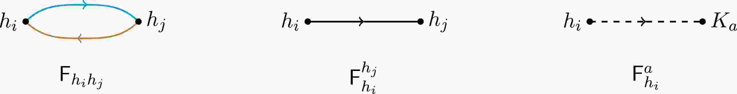
$ \dim{\cal W}_{n+m,m} = \#({\rm{vectors}}) $ , as defined in (3.50). Hence, the set of vectors defined in (3.50) satisfies the required two conditions and could be chosen as an expansion basis for$ A^{{ \rm{EYM}}}_{n,m} $ in (2.9). In practice, we would prefer a basis with minimal dimensions; then, we can define the fundamental f-terms as$\tag{3.54} {\mathsf{F}}_{h_ih_j}: = \frac{k_1\cdot f_{h_i}\cdot f_{h_j}\cdot k_1}{(k_1\cdot k_{h_i})(k_1\cdot k_{h_j})}\; \; \; ,\; \; \; 1\leqslant i<j\leqslant m\; ,\; \; \; $

$\tag{3.55} {\mathsf{F}}_{h_i}^{h_j}: = \frac{k_1\cdot f_{h_i}\cdot k_{h_j}}{k_1\cdot k_{h_i}}\; \; \; ,\; \; \; i\in\{1,\ldots,m\}\; ,\; j\in\{1,\ldots,m\}/\{i\}\; ,\; \; \; $

$\tag{3.56} {\mathsf{F}}_{h_i}^{a}: = \frac{k_1\cdot f_{h_i}\cdot K_a}{k_1\cdot k_{h_i}}\; \; \; ,\; \; \; i\in \{1,\ldots,m\}\; ,\; a\in\{2,\ldots,n-1\}\; ,\; \; \; $

where
$ K_a: = \sum_{i = 2}^{a} k_i $ . The vectors in the expansion basis can be constructed from the above fundamental f-terms as$\tag{3.57} \prod\limits_{i = 1}^{p} {\mathsf{F}}_{h_{\alpha_{2i-1}}h_{\alpha_{2i}}}\prod\limits_{i = 1}^{q}{\mathsf{F}}_{h_{\beta_i}}^{h_{\beta'_i}}\prod\limits_{i = 1}^{r} {\mathsf{F}}_{h_{\gamma_i}}^{a_{\gamma_i}}\; \; \; ,\; \; \; p,q,r\in{\mathbb N}\; \; \; {\rm{and}}\; \; \; 2p+q+r = m\; ,\; \; \; $

with the convention
$\tag{3.58} \begin{array}{l} \alpha_{2i-1}<\alpha_{2i+1}\; \; \forall(1\leqslant i\leqslant p-1)\; \; \; ,\; \; \; \alpha_{2i-1}<\alpha_{2i}\; \; \forall(1\leqslant i\leqslant p) \\ \beta_i<\beta_{i+1}\; \; \forall(1\leqslant i\leqslant q-1)\; \; \; ,\; \; \; \gamma_i<\gamma_{i+1}\; \; \forall(1\leqslant i\leqslant r-1) \end{array} \; .\; \; \; $

They contribute to a complete set of the expansion basis, and a general EYM amplitude can be expanded into this basis as
$\tag{3.59} \begin{aligned}[b] A^{{\rm{EYM}}}_{n;m}(k_1,k_2,\ldots,k_n;{\bf{H}}) = &\sum\limits_{h_{\beta'_{1}}\in {\bf{H}}/\{h_{\beta_1}\}}\cdots \sum\limits_{h_{\beta'_{q}}\in {\bf{H}}/\{h_{\beta_q}\}} \sum\limits_{a_{\gamma_1} = 2}^{n-1}\cdots \sum\limits_{a_{\gamma_r} = 2}^{n-1} \sum\limits_{{\mathfrak{a}}\cup{{\mathfrak{b}}}\cup{{\mathfrak{c}}} = {\bf{H}}}{\mspace{-24mu}\; '}\; \; \; {\cal C}[{\mathsf{F}}_{h_{\alpha_1}h_{\alpha_2}}\cdots {\mathsf{F}}_{h_{\alpha_{2p-1}}h_{\alpha_{2p}}}{\mathsf{F}}_{h_{\beta_1}}^{h_{\beta'_1}}\cdots {\mathsf{F}}_{h_{\beta_q}}^{h_{\beta'_q}}{\mathsf{F}}_{h_{\gamma_1}}^{a_{\gamma_1}}\cdots{\mathsf{F}}_{h_{\gamma_r}}^{a_{\gamma_r}}] \\ & \times {\cal B}[{\mathsf{F}}_{h_{\alpha_1}h_{\alpha_2}}\cdots {\mathsf{F}}_{h_{\alpha_{2p-1}}h_{\alpha_{2p}}}{\mathsf{F}}_{h_{\beta_1}}^{h_{\beta'_1}}\cdots {\mathsf{F}}_{h_{\beta_q}}^{h_{\beta'_q}}{\mathsf{F}}_{h_{\gamma_1}}^{a_{\gamma_1}}\cdots{\mathsf{F}}_{h_{\gamma_r}}^{a_{\gamma_r}}]\; ,\; \; \; \end{aligned} $

where
$ {\bf{H}}/{h_i} $ is the set of gravitons excluding$ h_i $ , and the three sets$ {\mathfrak{a}} = \{h_{\alpha_1},\ldots,h_{\alpha_{2p}}\} $ ,$ {\mathfrak{b}} = \{h_{\beta_1},\ldots,h_{\beta_q}\} $ , and$ {\mathfrak{c}} = \{h_{\gamma_1},\ldots, $ $h_{\gamma_r}\} $ with$ 2p+q+r = m $ are a splitting of all gravitons.$ {\cal B}[\cdots] $ represents a particular vector in the expansion basis$ {\cal B} $ ,$ {\cal C}[\cdots] $ represents the coefficient of the corresponding vector, and the reduced summation$ \sum' $ runs over all possible splittings$ {\mathfrak{a}}\cup{\mathfrak{b}}\cup{\mathfrak{c}} = {\bf{H}} $ , where the prime denotes that terms with the index circle should be excluded. The more discussion of index circle can be found in [33]. We can see that all the information regarding polarization vectors$ \epsilon_{h_{\kappa}} $ is encoded in$ {\cal B} $ , as expected. -
We have defined the gauge invariant expansion basis, and the next step is to determine the expansion coefficients. As mentioned earlier, the EYM amplitude can be expanded schematically in the form,
$\tag{4.1} \begin{aligned}[b] A^{{ \rm{EYM}}}_{n,m}(1,2,\ldots,n;{\bf{H}}) =& (\; \; {\rm{Coefficients}}\; \; ) \\&\otimes (\; \; {\rm{Gauge}}\;{\rm{Invariant}}\;{\rm{Basis}}\; \; )\; ,\end{aligned} $

or more explicitly, as in (3.59). The expansion coefficients are linear combinations of Yang-Mills amplitudes
$ A^{{\rm{YM}}}_{n+m} $ . To use (4.1) efficiently, a crucial point is to find a way to distinguish vectors in the gauge invariant basis from each other. Inspired by the explicit form of vectors in (3.1), we note that the signature of vectors is the structure$ (\epsilon\cdot \epsilon)^p(\epsilon\cdot k)^q $ , where$ (\epsilon\cdot \epsilon) $ and$ (\epsilon\cdot k) $ could be linearly independent. This motivates us to consider two kinds of differential operators:$\tag{4.2} {{\cal T}}_{ah_ib}: = \frac{\partial}{\partial(\epsilon_{h_i}\cdot k_a)}-\frac{\partial}{\partial(\epsilon_{h_i}\cdot k_b)}\; \; \; ,\; \; \; {{\cal T}}_{ab}: = \frac{\partial}{\partial(\epsilon_a\cdot \epsilon_b)}\; .\; \; \; $

Applying these operators to the RHS of (4.1), all terms will vanish except those containing corresponding
$ (\epsilon\cdot \epsilon) $ and$ (\epsilon\cdot k) $ . While applying these operators to the LHS of (4.1), the physical meaning will be different. Applying$ {{\cal T}}_{ab} $ to single-trace EYM amplitudes produces multi-trace EYM amplitudes, which would complicate the amplitude expansion; however, applying$ {\cal T}_{ah_i b} $ to a single-trace EYM amplitude produces another single-trace EYM amplitude but with one less graviton.$ {\cal T}_{ah_i b} $ will transform the graviton$ h_i $ to a gluon$ h_i $ and insert the gluon in the positions between gluons$ a, b $ respecting the color-ordering. Therefore, each time an insertion operator is applied to (4.1), the number of gravitons is reduced by one; then, a multiplication of m insertion operators would transform the LHS of (4.1) to Yang-Mills amplitudes completely, as expected ⑭.In fact, we can take one step further and define a differential operator as a multiplication of m properly chosen insertion operators. When applying the differential operator to (3.59), in addition to some vectors with already known coefficients, there would be one and only one vector with unknown coefficient remaining in the RHS of (3.59), and all other vectors vanish:
$\tag{4.3}\begin{aligned}[b] &{\rm{Differential}}\;{\rm{Operator}}\;{\rm{on}}\; A^{{ \rm{EYM}}}_{n,m} = {\rm{Coefficient}}\\&\quad\times (\; \; {\rm{Differential}}\;{\rm{Operator}}\;{\rm{on}}\; {\cal B}\; \; )\; .\end{aligned} $

As a consequence, we have a linear equation with only one unknown variable, and the corresponding expansion coefficient can be computed directly as a function of
$ A^{{\rm{YM}}}_{n+m} $ , generated by a differential operator applied to the RHS of (3.59) ⑮. The problem of EYM amplitude expansion is then translated to construction of properly defined differential operators, which would be the major purpose of this section. Surprisingly, we find it very helpful to use quivers to represent the gauge invariant basis and differential operators for our purpose. -
The definition of insertion operator (4.2) indicates that a differential operator would only affect the Lorentz contraction
$ (\epsilon_{h}\cdot k) $ , so all other types of Lorentz contractions$ (k\cdot k) $ and$ (\epsilon\cdot \epsilon) $ can be treated as unrelated factors. To characterize the structure of$ (\epsilon_h\cdot k) $ in a gauge invariant vector, we can assign a quiver, i.e., directed graph, to it⑯. Therefore, in this subsection, we first define the quiver representation of atomic factors such as$ (\epsilon_i\cdot k_j) $ ; second, we give the quiver representations of fundamental f-terms; finally, we consider the quiver representation of gauge invariant vectors and discuss the properties of their quiver representation.We call a directed graph representing all
$ (\epsilon\cdot k) $ of a vector the$ (\epsilon k) $ -quiver of the vector. In a quiver, we use a directed solid line to represent$ (\epsilon_{h_i}\cdot k_{h_j}) $ with an arrow pointing to a graviton momentum$ k_{h_i} $ and a directed dashed line to represent$ (\epsilon_{h_i}\cdot k_j) $ with an arrow pointing to a gluon momentum$ k_j $ , as [45], [46] ⑰As for the fundamental f-term (3.48), which can be expanded as
$\tag{4.4} \begin{align} k_1\cdot f_{h_i}\cdot f_{h_j}\cdot k_1& = (k_1\cdot k_{h_i})(\epsilon_{h_i}\cdot k_{h_j})(\epsilon_{h_j}\cdot k_1) -(k_1\cdot k_{h_i})(\epsilon_{h_i}\cdot \epsilon_{h_j})(k_{h_j}\cdot k_1) \\ &\; \; \; \; \; \; \; \; \; \; \; \; -(k_1\cdot \epsilon_{h_i})(k_{h_i}\cdot k_{h_j})(\epsilon_{h_j}\cdot k_1)+(k_1\cdot \epsilon_{h_i})(k_{h_i}\cdot \epsilon_{h_j})(k_{h_j}\cdot k_1)\; ,\; \; \; \end{align} $

its
$ (\epsilon k) $ -quiver representation consists of three$ (\epsilon k) $ -directed graphs, as ⑱Because each graph denotes a multiplication of
$ (\epsilon\cdot k) $ terms, when applying the derivatives$\tag{4.6} \frac{\partial}{\partial (\epsilon_{h_i}\cdot k_1)}\frac{\partial}{\partial (\epsilon_{h_j}\cdot k_1)}\; \; \; ,\; \; \; \frac{\partial}{\partial (\epsilon_{h_j}\cdot k_{h_i})}\frac{\partial}{\partial (\epsilon_{h_i}\cdot k_1)}\; \; \; , \frac{\partial}{\partial (\epsilon_{h_i}\cdot k_{h_j})}\frac{\partial}{\partial (\epsilon_{h_j}\cdot k_1)} $

to
$ (k_1\cdot f_{h_i}\cdot f_{h_j}\cdot k_1) $ , we will get non-vanishing results. Similarly, for$ (k_1\cdot f_{h_i}\cdot k) $ , their$ (\epsilon k) $ -quivers arewhere we have distinguished two cases,
$ k_{h_j} $ being the momentum of a graviton$ h_j $ and$ k_j $ being a momentum of a gluon.Note that the factor
$ (\epsilon_{h_i}\cdot k_1) $ exists in both$ (k_1\cdot f_{h_i}\cdot f_{h_j}\cdot k_1) $ and$ (k_1\cdot f_{h_i}\cdot k) $ , so the action of the derivative$ \partial_{\epsilon_{h_i}\cdot k_1} $ on them both is non-zero. Consequently, we prefer to eliminate the dashed lines representing$ \epsilon_{h_i}\cdot k_1 $ in the graphs of$ (\epsilon k) $ -quivers to obtain a simple presentation. Furthermore, to represent one fundamental f-term by only one graph and distinguish$ {\mathsf{F}}_{h_ih_j} $ from$ {\mathsf{F}}_{h_i}^{h_j} $ , we combine the two solid arrows in (4.5) into a loop. Finally, the fundamental f-terms$ {\mathsf{F}}_{h_ih_j} $ ,$ {\mathsf{F}}_{h_i}^{h_j} $ ,$ {\mathsf{F}}_{h_i}^a $ defined in (3.54), (3.55), and (3.56) are represented by quivers in Fig. 1. To distinguish these quivers from$ (\epsilon k) $ -quivers, we will call them basis quivers or just quivers.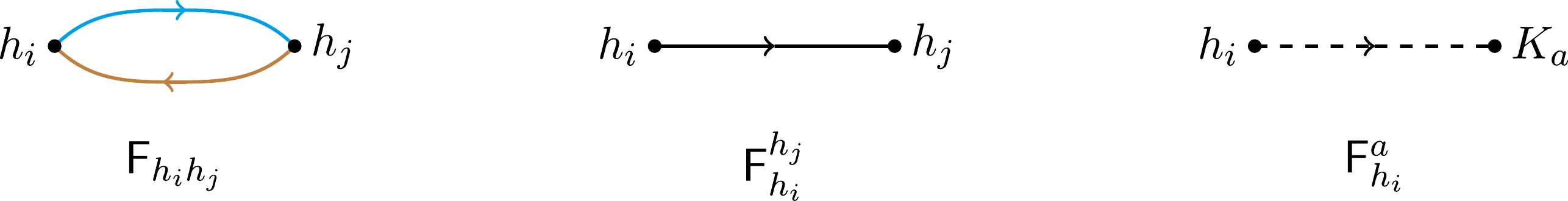
Figure 1. (color online) Quiver representation of fundamental f-terms.
We should emphasize that from a basis quiver, it is easy to recover all corresponding
$ (\epsilon k) $ -quivers by replacing any one solid or dashed arrow$ (\epsilon_{h_i}\cdot k) $ in the graph by a dashed arrow$ (\epsilon_{h_i}\cdot k_1) $ , i.e., from Fig. 1 to (4.5), (4.7). However, given an$ (\epsilon k) $ -quiver, it is difficult to determine which basis quiver it comes from, especially when there are many$ (\epsilon\cdot k_1) $ lines. The fact that there is no one-to-one correspondence between basis quivers and$ (\epsilon k) $ -quivers causes some technical difficulties in the construction of differential operators. Fortunately, for a gauge invariant vector, its basis quiver and$ (\epsilon k) $ -quivers do possess a common property: they all contain m and only m lines (counting both dashed lines and solid lines), as each line carries one$ \epsilon_{h_i} $ .Note that the basis quiver for
$ {\mathsf{F}}_{h_ih_j} $ is a colored loop, where the colors are to remind us that it is an overlapping of three$ (\epsilon k) $ -quivers after eliminating dashed lines. We call such a colored loop a pseudo-loop. In general, there are also real loops. For example, the$ {\mathsf{F}}_{h_1}^{h_2}{\mathsf{F}}_{h_2}^{h_1} $ containing a monomial$ (\epsilon_{h_1}k_{h_2})(\epsilon_{h_2}k_{h_1}) $ and$ {\mathsf{F}}_{h_1}^{h_2}{\mathsf{F}}_{h_2}^{h_3}{\mathsf{F}}_{h_3}^{h_1}{\mathsf{F}}_{h_4}^{h_3} $ containing a monomial$ (\epsilon_{h_1}k_{h_2})(\epsilon_{h_2}k_{h_3})(\epsilon_{h_3}k_{h_1})(\epsilon_{h_4}k_{h_3}) $ can be represented asHowever, as explained in [33], the terms with indices or part of indices forming a closed circle will not be present in the expansion of the EYM amplitude, although such terms do appear in the gauge invariant basis. Therefore, we will exclude basis quivers with real loops in practical computation.
Next, let us consider the quiver representation of a vector in the gauge invariant basis. As shown in (3.57), such a vector is a multiplication of fundamental f-terms, expressed as
$\tag{4.8} \left( \prod\limits_{i = 1}^{p} {\mathsf{F}}_{h_{\alpha_{2i-1}}h_{\alpha_{2i}}}\right) \left(\prod\limits_{i = 1}^{q}{\mathsf{F}}_{h_{\beta_i}}^{h_{\beta'_i}}\right) \left( \prod\limits_{i = 1}^{r} {\mathsf{F}}_{h_{\gamma_i}}^{a_{\gamma_i}}\right)\; .\; \; \; $

Because each
$ \epsilon_{h_i} $ appears only once in a vector, only one$ (\epsilon_{h_i}\cdot k) $ exists; therefore, we can conclude that each point labelled by$ h_i $ in the basis quiver of a gauge invariant vector has at most one out-going line but possibly several in-coming lines. Consequently, all pseudo-loops are topologically disconnected from each other. The point labelled by$ K_a $ is connected by only in-coming lines but not out-going lines; hence, all such points are also topologically disconnected from each other. Furthermore, pseudo-loops cannot be connected with points labelled by$ K_a $ either. Therefore, a quiver graph could have many disconnected components, whose number is at least p and at most$ p+r $ , as several dashed lines can be connected to the same node$ K_{a_i} $ , while a solid line for$ {\mathsf{F}}_{h_i}^{h_j} $ can be connected to one and only one disconnected component.With the above analysis, let us discuss the possible structures appearing in a quiver representation for a vector in a gauge invariant basis (4.8). First, because each
$ {\mathsf{F}}_{h_{\gamma_i}}^{a_{\gamma_i}} $ is represented by a dashed directed line with an arrow pointing to$ K_{a_{\gamma_i}} $ , its head can never be connected with a pseudo-loop or a solid line. Second, each$ {\mathsf{F}}_{h_{\beta_i}}^{h_{\beta'_i}} $ is represented by a solid line with an arrow pointing to$ h_{\beta'_i}\neq h_{\beta_i} $ , so if$ h_{\beta'_i}\in $ $ \{h_{\gamma_1},\ldots, h_{\gamma_r}\} $ , its head is linked with a dashed line, while if$ h_{\beta'_i}\in \{h_{\alpha_1},\ldots,h_{\alpha_{2p}}\} $ , its head is linked with a pseudo-loop, and if$ h_{\beta'_i}\in \{h_{\beta_1},\ldots, h_{\beta_r}\}/\{h_{\beta_{i}}\} $ , for instance$ h_{\beta'_i} = h_{\beta_j} $ , its head is linked with another solid line, and the head of the latter is further linked with a pseudo-loop, a dashed line, or a solid line. A succession of solid lines should finally stop at a dashed line or a pseudo loop; otherwise, it would form a real loop that should be excluded.To summarize, the quiver representation of a vector in a gauge invariant basis could contain the following sub-structures:
1. only a single dashed line,
2. a dashed line linked with a tree consisting of solid lines,
3. only a single pseudo-loop,
4. a pseudo-loop connected to a tree consisting of solid lines on one side,
5. a pseudo-loop connected to two trees consisting of solid lines on both sides,
as shown in Fig. 2. Two examples of quiver representations for two vectors in the gauge invariant basis of
$ A^{{ \rm{EYM}}}_{n,6} $ are shown as follows: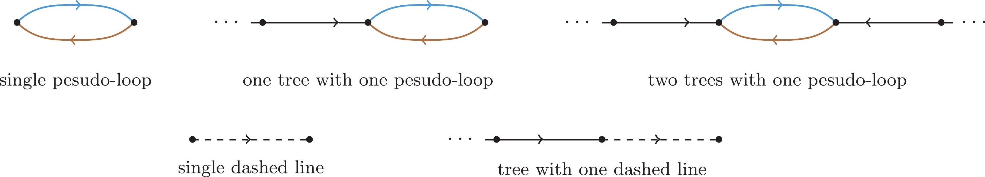
Figure 2. (color online) Possible structures that can appear in the quiver representation of a gauge invariant basis. The solid line without a starting point denotes possible tree or line segments. The dashed lines could be connected at the same point
$ K_a $ .The two examples illustrate our previous discussion very well. There are three disconnected components for the first one and two for the second one. In the second graph, two dashed lines are connected to one node, representing the fundamental f-terms
$ {\mathsf{F}}_{h_3}^{4} $ ,$ {\mathsf{F}}_{h_6}^{4} $ . All directed solid lines stop at pseudo-loops or dashed lines.In fact, we can give a more precise description of the structures of basis quivers using the concept of a rooted tree [47]. The quiver of a vector in a gauge invariant basis consists of some disconnected components, and each component contains only one pseudo-loop or a node
$ K_{a_i} $ . If we focus on a disconnected component with node$ K_{a_i} $ , it is exactly a rooted tree, with the root being the node$ K_{a_i} $ . More precisely, it is a directed rooted tree with an orientation toward the root, i.e., all lines in the tree are directed to the root from the leaves, as illustrated in the previous two examples. For the disconnected component with a pseudo-loop, we could split the pseudo-loop into two colored lines, resulting in two sub-graphs. For each sub-graph, we take the node with only in-coming lines as the root; thus, we obtain two rooted trees from a disconnected component with a pseudo-loop. This picture of rooted trees will help us to construct the differential operators and understand many properties of our algorithm later. -
Because a vector in the gauge invariant basis is a polynomial of
$ (\epsilon\cdot k) $ , it will be non-vanishing under the action of a derivative$ \partial_{\epsilon_{h_i}\cdot k} $ only if its$ (\epsilon k) $ -quiver representation contains a solid or dashed line corresponding to$ \epsilon_{h_i}\cdot k $ . Hence, by constructing a differential operator as a proper combination of some derivatives$ \partial_{\epsilon_{h_i}\cdot k} $ , we expect under its action that ideally only one vector is non-vanishing, so it can select a particular non-vanishing vector in a gauge invariant basis. Although in fact we cannot do this, we succeed in dividing the computation of coefficients of a gauge invariant basis into many steps, and in each step, by applying an appropriate differential operator, only one new vector is non-vanishing, except some vectors whose coefficients are already known. The goal in this subsection is to construct such differential operators.The expected differential operators can be constructed using three types of insertion operators (4.1). The first type of insertion operator takes the form
$\tag{4.10} {\cal T}_{ah_i(a+1)} = \partial_{\epsilon_{h_i}\cdot k_a}-\partial_{\epsilon_{h_i}\cdot k_{a+1}}\; \; \; ,\; \; \; a = 2,3,\ldots, n-1\; ,\; \; \; $

where
$ k_a $ is the momentum of a gluon. A vector is non-zero under$ {\cal T}_{ah_i(a+1)} $ if its$ (\epsilon k) $ -quiver contains a dashed line corresponding to$ \epsilon_{h_i}\cdot k_a $ or$ \epsilon_{h_i}\cdot k_{a+1} $ . Applying this insertion operator to the fundamental f-terms, we have$ \tag{4.11} {\cal T}_{ah_i(a+1)}\; {\mathsf{F}}_{h_{\alpha_{2j-1}}h_{\alpha_{2j}}} = 0\; \; \; ,\; \; \; {\cal T}_{ah_i(a+1)}\; {\mathsf{F}}_{h_{\beta_j}}^{h_{\beta'_j}} = 0\; ,\; \; \; $

and
$\tag{4.12} {\cal T}_{a h_i (a+1)}\; {\mathsf{F}}_{h_j}^b = \left[\partial_{(\epsilon_{h_i}\cdot k_a)}-\partial_{(\epsilon_{h_i}\cdot k_{a+1})}\right]\sum\limits_{l = 2}^{b}\frac{(k_1\cdot k_{h_j})(\epsilon_{h_j}\cdot k_l)-(k_1\cdot \epsilon_{h_j})(k_{h_j}\cdot k_l)}{k_1\cdot k_{h_j}} = \delta_{ij}\delta_{ab}\; .\; \; \; $

The above results tell us that if the basis quiver of a vector in a gauge invariant basis contains a dashed line representing
$ {\mathsf{F}}_{h_{\gamma_i}}^a $ , then a differential operator containing the insertion operator$ {\cal T}_{a h_i (a+1)} $ will select out this vector and other vectors containing the same dashed line. The relation (4.12) can be graphically represented as,The second type of insertion operator takes the form
$ {\cal T}_{h_jh_in} = \partial_{\epsilon_{h_i}\cdot k_{h_j}}-\partial_{\epsilon_{h_i}\cdot k_n} $ , where the Lorentz contraction of a polarization vector with a graviton momentum has been included. Because by definition the momentum$ k_n $ does not appear in the fundamental f-terms, when applying$ {\cal T}_{h_jh_in} $ to them, only the derivative$ \partial_{\epsilon_{h_i}\cdot k_{h_j}} $ works. Explicitly, we have$\tag{4.14}\begin{aligned}[b] &{\cal T}_{h_jh_in}\; {\mathsf{F}}_{h_i'}^{a_{i'}} = 0\; ,\; \; \; {\cal T}_{h_jh_in}\; {\mathsf{F}}_{h_{i'}}^{h_{j'}} = \delta_{ii'}\delta_{jj'}\; ,\\& {\cal T}_{h_jh_in}\; {\mathsf{F}}_{h_{i'}h_{j'}} = \frac{\epsilon_{h_j}\cdot k_1}{k_1\cdot k_{h_j}} \left( \delta_{ii'}\delta_{jj'}+\delta_{ij'}\delta_{ji'} \right) ,\; \; \; \end{aligned} $

represented in quivers as
Because both
$ {\mathsf{F}}_{h_ih_j} $ and$ {\mathsf{F}}_{h_i}^{h_j} $ are non-vanishing under$ {\cal T}_{h_jh_in} $ , we may conclude that this insertion operator is not sufficient to distinguish these two terms. However, we shall note that the insertion operator is actually a differential operator that works through the smaller pieces, i.e., Lorentz contractions$ (\epsilon_{h_i}\cdot k_j) $ , rather than the fundamental f-terms$ {\mathsf{F}}_{h_ih_j} $ and$ {\mathsf{F}}_{h_i}^{h_j} $ . According to this view, it is easy to accept that$ {\mathsf{F}}_{h_ih_j} $ and$ {\mathsf{F}}_{h_i}^{h_j} $ are non-vanishing under the action of$ {\mathsf{F}}_{h_ih_j} $ , as their quivers both contain a solid line from$ h_i $ to$ h_j $ .To construct a differential operator that can distinguish
$ {\mathsf{F}}_{h_ih_j} $ from$ {\mathsf{F}}_{h_i}^{h_j} $ , we need to consider a third type of composite insertion operator. The key difference in these two terms is that$ {\mathsf{F}}_{h_ih_j} $ has two polarization vectors, while$ {\mathsf{F}}_{h_i}^{h_j} $ has only one. In other words, in the$ (\epsilon k) $ -quiver of$ {\mathsf{F}}_{h_ih_j} $ , there are always two lines linked together, a solid line$ (h_i h_j) $ and a dashed line$ (1 h_i) $ or$ (1 h_j) $ , so we can multiply$ {\cal T}_{h_jh_in} $ by an additional insertion operator containing the derivative$ {{\rm{d}}}_{\epsilon_{h_j}\cdot k_1} $ ; under such operators,$ {\mathsf{F}}_{h_i}^{h_j} $ always vanishes. Then, choosing the operator$ {\cal T}_{1h_j2}{\cal T}_{h_jh_in} $ and applying it to$ {\mathsf{F}}_{h_ih_j} $ , we have$\tag{4.15} (k_1\cdot k_{h_j}){\cal T}_{1h_j2}{\cal T}_{h_jh_in}\; {\mathsf{F}}_{h_{i'}h_{j'}} = \delta_{ii'}\delta_{jj'}\; .\; \; \; $

It is easy to see that the operator satisfies our requirement for distinguishing
$ {\mathsf{F}}_{h_ih_j} $ and$ {\mathsf{F}}_{h_i}^{h_j} $ , and it also distinguishes the pseudo-loop of$ {\mathsf{F}}_{h_{i}h_{j}} $ from all other pseudo-loops. However$ {\cal T}_{1h_j2} $ causes some additional difficulty, as there will be some multiplication of fundamental f-terms that do ont vanish, such as ⑲$\tag{4.16} \begin{aligned}[b]& (k_1\cdot k_{h_j}){\cal T}_{1h_j2}{\cal T}_{h_jh_in}{\mathsf{F}}_{h_i}^{h_j}{\mathsf{F}}_{h_j}^{a_t} = -k_{h_j}\cdot (k_1+K_{a_t})\; \; \;,\\& (k_1\cdot k_{h_j}){\cal T}_{1h_j2}{\cal T}_{h_jh_in}{\mathsf{F}}_{h_i}^{h_j}{\mathsf{F}}_{h_j}^{h_p} = -k_{h_j}\cdot k_{h_p}\; .\; \; \; \end{aligned} $

This means that although
$ {\cal T}_{1h_j2}{\cal T}_{h_jh_in} $ is able to distinguish one pseudo-loop from the others, it would mix contributions from vectors without pseudo-loops. However, this is not a problem at all, if we attempt to solve the coefficients of the basis in multiple steps. We can first compute the coefficients of$ {\mathsf{F}}_{h_i}^{h_j}{\mathsf{F}}_{h_j}^{a_j} $ and$ {\mathsf{F}}_{h_i}^{h_j}{\mathsf{F}}_{h_j}^{h_p} $ using the differential operators$ {\cal T}_{a_jh_j(a_j+1)}{\cal T}_{h_jh_in} $ and$ {\cal T}_{h_p h_j n}{\cal T}_{h_jh_in} $ respectively, under which$ {\mathsf{F}}_{h_ih_j} $ has no contribution at all. Then, we can apply$ {\cal T}_{h_jh_in}{\cal T}_{1h_j2} $ to compute the coefficient of$ {\mathsf{F}}_{h_ih_j} $ , and we treat the coefficients of$ {\mathsf{F}}_{h_i}^{h_j}{\mathsf{F}}_{h_j}^{a_j} $ ,$ {\mathsf{F}}_{h_i}^{h_j}{\mathsf{F}}_{h_j}^{h_p} $ as known input.After the above discussion, we can roughly give a general picture of constructing a differential operator to select a particular vector in the gauge invariant basis through the quiver representation. The major idea is to construct a new special
$ (\epsilon k) $ -quiver from a vector's basis quiver, which can be used to construct the expected differential operators. A reasonable method for determining these new$ (\epsilon k) $ -quivers is as follows: a dashed line in the basis quiver of a vector suggests that there is also a dashed line in the new$ (\epsilon k) $ -quiver, but representing$ (\epsilon_{h_i}\cdot K_a) $ and a solid line$ (h_i h_j) $ in the basis quiver also suggests that there is a solid line in the new$ (\epsilon k) $ -quiver representing$ (\epsilon_{h_i}\cdot k_{h_j}) $ , while for a pseudo-loop in the basis quiver, we can choose to construct either a solid line$ (\epsilon_{h_i}\cdot k_{h_j}) $ connected to a dashed line$ (\epsilon_{h_j}\cdot k_1) $ or a solid line$ (\epsilon_{h_j}\cdot k_{h_i}) $ connected to a dashed line$ (\epsilon_{h_i}\cdot k_1) $ in the new$ (\epsilon k) $ -quiver. We are free to take any one of the two choices when meeting a pseudo-loop. Finally, we obtain a new$ (\epsilon k) $ -quiver, which is used to construct differential operators.As we discussed at the end of the previous subsection, the
$ (\epsilon k) $ -quiver is a collection of rooted trees. The disconnected component of a pseudo-loop in the basis quiver of a vector has been split into two branches, where each branch is a rooted tree with the root being$ k_1 $ and is suitable according to our choice, and the components without pseudo-loops directly give us rooted trees. Furthermore, a collection of rooted trees can be algebraically represented as an embedded structure, where at each level, we write$\{ {\rm{root}}:{\rm{leaf}}\;{\rm{1}};...;{\rm{leaf}}\;{\rm{m}}\} $ .⑳Second, having obtained the desired
$ (\epsilon k) $ -quivers, we can construct the corresponding differential operators using the following rules:1. assign an operator
$ {\cal T}_{a h_i(a+1)} $ to each dashed line$ (h_i K_a) $ in the new$ (\epsilon k) $ -quiver, which uniquely picks up the corresponding dashed line in a vector's basis quiver;2. assign an operator
$ {\cal T}_{h_jh_in} $ to each solid line$ (h_i h_j) $ in the new$ (\epsilon k) $ -quiver, which uniquely picks up the corresponding solid line in a vector's basis quiver;3. assign an operator
$ (k_1\cdot k_{h_i}){\cal T}_{1 h_i 2} $ to each dashed line$ (h_ik_1) $ in the new$ (\epsilon k) $ -quiver.These rules can be represented graphically as
Therefore, the corresponding differential operator for a vector in a gauge invariant basis is defined by multiplying all assigned operators in the new
$ (\epsilon k) $ -quiver together; then, we call the$ (\epsilon k) $ -quivers constructed according to the above rules D-quivers. We want to emphasize the following: (1) there is a one-to-one map between D-quivers and differential operators, so one quiver defines a unique differential operator; (2) a D-quiver is a special$ (\epsilon k) $ -quiver, which can be associated with a given basis quiver.Finally, the above discussion can be summarized as the following map, stating that from a given vector to a corresponding differential operator,
$\tag{4.19} \begin{aligned} B_i = \left( \prod\limits_{i = 1}^{p} {\mathsf{F}}_{h_{\alpha_{2i-1}}h_{\alpha_{2i}}}\right) \left(\prod\limits_{i = 1}^{q}{\mathsf{F}}_{h_{\beta_i}}^{h_{\beta'_i}}\right) \left( \prod\limits_{i = 1}^{r} {\mathsf{F}}_{h_{\gamma_i}}^{a_{\gamma_i}}\right) \to D_i = \left( \prod\limits_{i = 1}^{p} (k_1\cdot k_{h_{\alpha_{2i}}}) {\cal T}_{h_{\alpha_{2i}}h_{\alpha_{2i-1}}n}{\cal T}_{1h_{\alpha_{2i}}2}\right) \left(\prod\limits_{i = 1}^{q} {\cal T}_{h_{\beta'_{i}}h_{\beta_{i}}n}\right) \left( \prod\limits_{i = 1}^{r} {\cal T}_{a_{\gamma_i}h_{\gamma_{i}}(a_{\gamma_i+1})}\right)\; ,\; \; \; \end{aligned} $

where
$ B_i\in {\cal B} $ . There are several technical points we wish to explain. First, the mapping rule is defined such that$\tag{4.20} \begin{array}{l} D_i[B_i] = 1\; .\; \; \; \end{array} $

Second, although insertion operators are commutative, when acting on EYM amplitudes, we need to choose a proper order to make the physical meaning clear. We shall apply insertion operators of the type
$ {\cal T}_{ah_{\gamma}a'}, {\cal T}_{1h_\alpha 2} $ first; then, we apply the types$ {\cal T}_{h_\alpha h_{\alpha}' n} $ and$ {\cal T}_{h_{\beta}h_\beta' n} $ . More explicitly, the ordering of applying insertion operators is from the roots to the leaves in the D-quiver opposite to the direction of the arrows.In fact, we can make the result more concrete when acting
$ D_i $ on$ A^{\rm EYM}_{n,m} $ . As mentioned, each$ D_i $ can be represented by a D-quiver as a collection of rooted trees. For example, the D-quiver for a differential operator isThen, the rooted trees can be written as
$\tag{4.21} \begin{aligned}[b]& \{k_1:\{h_1: \{h_2, h_4\}; h_3\}; \{h_5, h_6\}\} ,\\& \{K_4:\; h_8;\; \{h_9, h_{10}: h_{11}; h_{12}\}\} ,\;\;\{K_6: h_7\} .\; \end{aligned} $

Applying this to
$ A^{{ \rm{EYM}}}_{n,12} $ leads to$\tag{4.22} \begin{aligned}[b] & A^{{\rm{YM}}}_{n+12}\big(1, \; \; \{ h_1, \{h_2, h_4\}\shuffle h_3\}\; \; \shuffle \; \; \{h_5, h_6\}\; \; \\ & \quad \shuffle \; \; \{2,3,4,\; h_8\; \shuffle\; \{h_9, h_{10},h_{11}\shuffle h_{12}\}\; \\&\quad\shuffle \; \{5,6, \; h_7\; \shuffle\; \{7,...,n-1\}_R\; \; \}_R\; \; \}_R,\; \; n \big)\; ,\; \; \; \end{aligned} $

multiplied by
$ (k_1\cdot k_{h_1})(k_1\cdot k_{h_5}) $ . This example contains all crucial points we wish to clarify, so let us give more explanation, especially about the similarity between the shuffle structure in (4.22) and the rooted tree structure in (4.21).● First, let us consider the tree with root
$ k_1 $ . It is connected to two branches,$ \{h_1: \{h_2, h_4\}; h_3\} $ and$ \{h_5, h_6\} $ . Applying$ {\cal T}_{1h_{1}2} $ and$ {\cal T}_{1h_{5}2} $ will produce the structure$\tag{4.23} \begin{array}{l} A(1, \{h_1\} \shuffle \{h_5\} \shuffle\{2,3,...,n-1\}_R, n)\; ,\; \; \; \end{array} $

where the subscript R denotes a "restricted shuffle," meaning that when making a shuffle permutation for three sets, the first element of the third set should be placed after the first element of the other two sets. Applying
$ {\cal T}_{h_{5} h_6 n} $ from the first branch will give us$ \{h_5,h_6\} $ , as$\tag{4.24} \begin{array}{l} A(1, \{h_1\} \shuffle \{h_5,h_6\} \shuffle\{2,3,...,n-1\}_R, n)\; ,\; \; \; \end{array} $

while applying insertion operators from the second branch will give
$ \{h_1, \; \{h_2, h_4\}\shuffle \;h_3\} $ , as$\tag{4.25} A^{\rm{YM}}_{n+12}\left(1, \; \{ h_1, \{h_2, h_4\}\shuffle h_3\} \shuffle \{h_5, h_6\} \shuffle \; \; \{2,3,...,n-1\}_R,\; n \right) .$

● Second, let us consider the rooted tree with root
$ K_4 $ , which also contains two branches. Applying$ {\cal T}_{4h_{8}5} $ and$ {\cal T}_{4h_{9}5} $ on the sub-structure$ \{2,3,...,n-1\}_R $ in (4.25) results in$\tag{4.26} \begin{aligned}[b] & A^{\rm{YM}}_{n+12}\big(1, \; \; \{ h_1, \{h_2, h_4\}\shuffle h_3\}\; \; \shuffle \; \; \{h_5, h_6\}\; \; \\ &\quad \shuffle \; \; \{2,3,4,h_8\shuffle\{h_9, h_{10},h_{11}\shuffle h_{12}\}\\&\quad\shuffle \{5,6,...,n-1\}_R\; \; \}_R,\; \; n \big)\; .\; \; \; \end{aligned} $

● Finally, let us consider the remaining tree structure
$ \{K_6: h_7\} $ with root$ K_6 $ . Applying$ {\cal T}_{6h_{7}7} $ on the sub-structure$ \{5,6,...,n-1\}_R $ in (4.26) will give us$ \{5,6, h_7\shuffle$ $ \{7,...,n-1\}_R\; \; \}_R $ , just as shown in (4.22). -
Having defined the corresponding differential operator
$ D_i $ for a vector in a gauge invariant basis as in (4.19), we can apply it to equation (4.1) and obtain a linear equation for the expansion coefficient of a particular$ B_i $ , as well as other coefficients. However, for a vector with pseudo-loops, in general, we will meet$ D_i[B_j]\neq 0 $ for some$ j\neq i $ . In this case, we have a set of linear equations. For an EYM amplitude with a large number of gravitons and gluons, the number of linear equations will become too large to be easily solved. Thus, it is better to find a way to avoid solving a large number of linear equations.To find a such method, we need to analyze the behaviors of different
$ B_j $ under the action of$ D_i $ , i.e., equations$ D_i[B_j]\neq 0 $ with different$ B_j $ under the same$ D_i $ . By inspecting D-quivers and corresponding operators, we find that there are two types of problems that cause difficulties in solving linear equations.The first problem comes from a key observation that, while operator
$ {\cal T}_{a h_i(a+1)} $ or$ {\cal T}_{h_jh_in} $ is able to select a particular dashed line or solid line uniquely in the basis quiver, the operator$ (k_1\cdot k_{h_i}){\cal T}_{1 h_i 2} $ fails to do so. As a consequence, the contributions of different basis quivers will mix together when they can produce the same D-quivers. The reason for this is that each pseudo-loop of the vectors' basis quiver has two possible ways of generating D-quivers, so it is possible that two basis quivers with pseudo-loops generate the same D-quiver. For example, let us consider the following four basis quivers$ B_i $ , which generate five D-quivers in total.Hence, if we choose
$ D_2 $ as the corresponding differential operator of the basis quiver$ B_1 $ , then after applying$ D_2 $ to these five vectors,$ B_2 $ is also non-zero, in addition to$ B_1 $ , which means that the coefficients of$ B_1, B_2 $ are mixed together in the linear equation given by$ D_2 $ .The above phenomenon is a general one. Assuming the basis quiver of a vector in the gauge invariant basis has a pseudo-loop
$ {\mathsf{F}}_{h_{\alpha_{2i-1}}h_{\alpha_{2i}}} $ connected with a solid line$ {\mathsf{F}}_{h_{\beta}}^{h_{{\alpha}_{2i}}} $ , and the corresponding differential operator of the pseudo-loop is$ (k_1\cdot k_{h_{\alpha_{2i}}}){\cal T}_{h_{\alpha_{2i}}h_{\alpha_{2i-1}}n}{\cal T}_{1h_{\alpha_{2i}}2} $ , then we can almost always find a new vector in the basis having a factor$ {\mathsf{F}}_{h_{{\beta}}h_{\alpha_{2i}}}{\mathsf{F}}_{h_{{\alpha}_{2i-1}}}^{h_{{\alpha}_{2i}}} $ ㉑, which is non-zero under the same differential operator. We can do this operation independently for each pseudo-loop in a vector. If there are$ \kappa_i $ solid lines connected to the node$ h_{{\alpha}_{2i}} $ , the total number of vectors that is non-zero under the corresponding differential operator of the pseudo-loop will be$ \left(\prod_{i = 1}^{p} (\kappa_i+1)-1\right) $ . The results of these vectors under the action of the differential operator are$ D_i[B_j] = 1 $ for$ B_j $ being a vector of the set; this fact will be important in the subsequent construction of a linear combination of$ D_i $ .Now, let us consider the second problem originating from identity (4.16). Although the basis quivers of some vectors will not produce the same D-quiver㉒, they could give the same
$ (\epsilon k) $ -quiver by replacing a dashed line$ (\epsilon\cdot K_a) $ or a solid line$ (\epsilon\cdot k_{h_j}) $ by$ (\epsilon\cdot k_1) $ . For example, applying$ D_1 $ to the following two basis quivers yields non-zero results,Note that
$ \widetilde{B_2} $ can be a rooted tree by itself or a rooted tree obtained by splitting a pseudo-loop, while$ \widetilde{B_1} $ can only be a rooted tree obtained by splitting a pseudo-loop. Thus, in this case, a branch of a disconnected component with a pseudo-loop is mixed with a disconnected component without a pseudo-loop. Explicitly, for a vector with a pseudo-loop$ {\mathsf{F}}_{h_{\alpha_{2i-1}}h_{\alpha_{2i}}} $ and the corresponding operator for the pseudo-loop$ (k_1\cdot k_{h_{\alpha_{2i}}}) {\cal T}_{h_{\alpha_{2i}}h_{\alpha_{2i-1}}n}{\cal T}_{1h_{\alpha_{2i}}2} $ , we can always find some new vectors by replacing$ {\mathsf{F}}_{h_{\alpha_{2i-1}}h_{\alpha_{2i}}} $ with$ {\mathsf{F}}_{h_{\alpha_{2i-1}}}^{h_{\alpha_{2i}}} {\mathsf{F}}_{h_{\alpha_{2i}}}^{K_a} $ ,$ \forall a = 2,...,n-1 $ or$ {\mathsf{F}}_{h_{\alpha_{2i-1}}}^{h_{\alpha_{2i}}} {\mathsf{F}}_{h_{\alpha_{2i}}}^{h_p} $ with arbitrary$ p\neq {\alpha}_{2i} $ ㉓. Because the replacement for each pseudo-loop is independent, there are a total of$ (2^p-1)(n-2+m-1) $ new vectors, and applying$ D_i $ to these new vectors would produce$ (-k_{h_{{\alpha}_{2i}}}\cdot (k_1+ K_a)) $ or$ (-k_{h_{{\alpha}_{2i}}}\cdot k_{h_p}) $ , respectively, according to (4.16). This is consistent with the counting of mass dimension. However, these new vectors have their corresponding differential operators (4.28) under which the original vector with a pseudo-loop vanishes. Thus, the second problem is easy to deal with if we solve the linear equations of unknown coefficients in the proper order.We have discussed two types of problems in detail, and the second type is easily solved, so let us continue to discuss how to deal with the first one. The first type of problem originates from the fact that under the action of a differential operator, several vectors with pseudo-loops in the gauge invariant basis do not vanish at the same time, so their coefficients are mixed together in the linear equations. Our solution is to construct a linear combination of differential operators such that under its action, only one vector is non-vanishing. Let us start from the simple example (4.27), where it is easy to get
$\tag{4.29} \begin{aligned}[b] D_2(b_1B_1+b_2B_2+b_3B_3+b_4B_4) = &b_1+b_2 , \\ D_3(b_1B_1+b_2B_2+b_3B_3+b_4B_4) =& b_2+b_3, \\ D_4(b_1B_1+b_2B_2+b_3B_3+b_4B_4) = & b_3+b_4 , \\ D_5(b_1B_1+b_2B_2+b_3B_3+b_4B_4) =& b_4 . \end{aligned} $

If we define some new differential operators as
$ {\cal D}_i : = \sum_{a = i}^{4}(-1)^{a-1}D_{a+1} $ , then$\tag{4.30}{\cal D}_i[B_j] = (-)^{i-1}\delta_{ij}\; \; \; ,\; \; \; i,j = 1,2,3,4\; .\; \; \;$

This means
$ {\cal D}_i $ selects a unique vector from the entangled vectors, and the linear equations of the coefficients of these vectors are easily solved. Generalizing this example, we can construct the linear combination of differential operators as follows.● For a given vector
$ B_i $ , we can obtain many D-quivers in general, but we choose only one D-quiver freely. For example,● For the D-quiver whose root is
$ k_1 $ , there are two nodes coming from the original pseudo-loop. If the node connected to$ k_1 $ by a dashed line is denoted$ h_{a} $ , then another node is denoted by$ h_{b} $ . We can separate this D-quiver into two parts in the node$ h_a $ while assigning the line connecting$ h_a $ and$ h_b $ to$ h_b $ , and denote these two parts by$ {\cal H}_a, {\cal H}_b $ . For example,● In graph
$ {\cal H}_a $ ,$ k_1 $ is connected to$ h_a $ , and$ k_1 $ is the root with all lines' directions toward$ k_1 $ . We can construct some new rooted trees by moving$ k_1 $ to other nodes and keeping$ h_a $ as the root; then, it is necessary to change the directions of lines. Each new rooted tree defines a differential operator denoted by$ D_{{\cal H}_a,j} $ with$ j = 1,...,k $ , where k is the total number of nodes excluding$ h_a $ in the rooted tree$ {\cal H}_a $ . Then, we define a new differential operator by$\tag{4.31} {\cal D}_{{\cal H}_a} = \sum\limits_{j = 1}^k (-)^{s(j)}D_{{\cal H}_a,j}\; ,\; \; \; $

where
$ s(j) $ is the number of steps for moving$ k_1 $ from the node$ h_a $ to the node$ h_j $ . For example,● Multiplying
$ {\cal D}_{{\cal H}_a} $ by the differential operator corresponding to$ {\cal H}_b $ gives us the expected operator, which will select only one particular vector from the set of vectors entangled with the original vector. For example, we get the linear combination● A basis quiver of a vector would have many disconnected components, and for each disconnected component with a pseudo-loop, we can apply the same procedure and similarly construct a corresponding operator
$ {\cal D} $ as a linear combination of some operators D. Multiplying all these operators$ {\cal D} $ with the operators obtained from disconnected components without pseudo-loops, we obtain the final differential operator, which will select a particular vector$ B_i $ in a gauge invariant basis without the first type of problem.We should emphasize that, after obtaining these differential operators using the above method, if we apply them to the expansion, there are still some issues resulting from the second type of problem. This suggests that we should solve coefficients of vectors with fewer pseudo-loops first. We also remark that, although we have provided the method to solve the problem of mixing of some vectors in solving the linear equations of coefficients, when the size of linear equations is small, it is quite favorable to solve them directly using the original differential operators defined in (4.19). The reason is that, while it is much simpler for computing coefficients of the mixed vectors by using differential operators constructed by the above method, it may be complicated for the cases we meet in the second type of problems since some vectors with less pseudo-loops are non-vanishing under the action of these operators for the second type of problems.
-
After clarifying the structure of differential operators, the next step is to apply them for computing the expansion coefficients for the generic expansion formula (3.59). For vectors of the gauge invariant basis defined in (3.57), the algorithm is implemented order by order, starting from
$ p = 0 $ to the largest value p. For a given p, we start from the largest r and proceed to$ r = 0 $ . The value of p denotes the number of pseudo-loops in a vector; hence, when$ p = 0 $ , the basis quiver contains only solid and dashed lines, without any pseudo-loops. Such a vector can be mapped to a unique D-quiver representing the following differential operator,$\tag{4.32} \left(\prod\limits_{i = 1}^{q} {\cal T}_{h_{\beta'_{i}}h_{\beta_{i}}n}\right) \left( \prod\limits_{i = 1}^{r} {\cal T}_{a_{\gamma_i}h_{\gamma_{i}}(a_{\gamma_i+1})}\right)\; \; ,\; \; q,r \in {\mathbb N}\; \; ,\; \; q+r = m\; .\; \; \; $

Recalling identities (4.11), (4.13), and (4.14), a vector
$ B_j $ is non-vanishing only when its$ D_j $ -quiver is the same as that given by (4.32). Thus, the differential operator (4.32) uniquely selects one vector in the gauge invariant basis while all others vanish, and the expansion coefficient can be solved using an univariate linear equation. Furthermore, the differential operator is normalized to one,$\tag{4.33} \left(\prod\limits_{i = 1}^{q} {\cal T}_{h_{\beta'_{i}}h_{\beta_{i}}n}\right) \left( \prod\limits_{i = 1}^{r} {\cal T}_{a_{\gamma_i}h_{\gamma_{i}}(a_{\gamma_i+1})}\right)\; \left[\; \left(\prod\limits_{i = 1}^{q}{\mathsf{F}}_{h_{\beta_i}}^{h_{\beta'_i}}\right) \left( \prod\limits_{i = 1}^{r} {\mathsf{F}}_{h_{\gamma_i}}^{a_{\gamma_i}}\right)\; \right] = 1\; ,\; \; \; $

and hence, the expansion coefficient can be directly computed by applying differential operator (4.32) on the EYM amplitude, leading to
$ \tag{4.34}\begin{aligned}[b] {\cal C}[{\mathsf{F}}_{h_{\beta_1}}^{h_{\beta'_1}}\cdots {\mathsf{F}}_{h_{\beta_q}}^{h_{\beta'_q}}{\mathsf{F}}_{h_{\gamma_1}}^{a_{\gamma_1}}\cdots {\mathsf{F}}_{h_{\gamma_r}}^{a_{\gamma_r}}] =& \left(\prod\limits_{i = 1}^{q} {\cal T}_{h_{\beta'_{i}}h_{\beta_{i}}n}\right) \left( \prod\limits_{i = 1}^{r} {\cal T}_{a_{\gamma_i}h_{\gamma_{i}}(a_{\gamma_i+1})}\right)\\&\times A^{{ \rm{EYM}}}_{n,m}(1,2,\ldots,n;h_1,\ldots, h_m)\; .\end{aligned} $

Note that
$ {\cal T}_{a_{\gamma_i}h_{\gamma_{i}}(a_{\gamma_i+1})} $ inserts$ h_{\gamma_i} $ between$ a_{\gamma_i} $ and$ a_{\gamma_i}+1 $ relative to the color-ordering, while$ {\cal T}_{h_{\beta'_{i}}h_{\beta_{i}}n} $ inserts$ h_{\beta_i} $ between n and another graviton$ h_{\beta'_i} $ . Hence, in the resulting Yang-Mills amplitudes, the legs$ h_i $ can never appear in the positions before$ 2 $ or after n, and all Yang-Mills amplitudes are in the BCJ basis with legs$ 1, 2, n $ fixed. An example of evaluating (4.34) has been discussed in (4.22).For the
$ p = 1 $ case, the differential operator for a vector with one pseudo-loop is defined as ㉔,$\tag{4.35}\begin{aligned}[b]& \left((k_1\cdot k_{\alpha_2}){\cal T}_{h_{\alpha_{2}}h_{\alpha_{1}}n}{\cal T}_{1h_{\alpha_{2}}2}\right) \left(\prod\limits_{i = 1}^{q} {\cal T}_{h_{\beta'_{i}}h_{\beta_{i}}n}\right) \left( \prod\limits_{i = 1}^{r} {\cal T}_{a_{\gamma_i}h_{\gamma_{i}}(a_{\gamma_i+1})}\right)\; \; \; ,\\&q,r \in {\mathbb N}\; \; ,\; \; q+r = m-2\; ,\end{aligned} $

with indices following convention (3.58), and the total number of differential operators is
$ \frac{m!}{2(m-2)!}(n+m-3)^{m-2}\; .\; \; \; $

In differential operators (4.35), the insertion operator
$ {\cal T}_{1h_{\alpha_2}2} $ will contribute a derivative$ \partial_{\epsilon_{h_{\alpha_2}}\cdot k_1} $ relating to momentum$ k_1 $ . In its quiver, there is only one branch with root$ k_1 $ , and as we have analyzed, applying these differential operators on vectors will produce non-zero results only if the D-quiver of vector contains only one or no branch with root$ k_1 $ . Therefore, all vectors with two or more pseudo-loops will vanish under (4.35). Furthermore, when applying (4.35) on vectors without a pseudo-loop, there could be a non-zero contribution. However, it is not an issue because all coefficients of such vectors have been solved a priori by differential operators (4.32), and they enter into the linear equations as known parameters.For vectors with one pseudo-loop, there are in general more than one vector that is non-vanishing under a specific differential operator (4.35), as shown in (4.29). Therefore, we need to apply a complete set of differential operators to generate an algebraic system of linear equations and solve the expansion coefficients from this algebraic system. Alternatively, we can also apply the differential operator constructed by rule (4.31), i.e., a special linear combination of differential operators in (4.35). Then, an expansion coefficient can be determined by a univariate linear equation again. Nevertheless, we can compute the coefficient of a vector with one pseudo-loop as
$\tag{4.36} \begin{aligned}[b] {\cal C}[{\mathsf{F}}_{h_{\alpha_1}h_{\alpha_2}}{\mathsf{F}}_{h_{\beta_1}}^{h_{\beta'_1}}\cdots {\mathsf{F}}_{h_{\beta_q}}^{h_{\beta'_q}}{\mathsf{F}}_{h_{\gamma_1}}^{a_{\gamma_1}}\cdots {\mathsf{F}}_{h_{\gamma_r}}^{a_{\gamma_r}}] =& \left\{ \sum \left((k_1\cdot k_{\alpha_2}){\cal T}_{h_{\alpha_{2}}h_{\alpha_{1}}n}{\cal T}_{1h_{\alpha_{2}}2}\right) \left(\prod\limits_{i = 1}^{q} {\cal T}_{h_{\beta'_{i}}h_{\beta_{i}}n}\right) \left( \prod\limits_{i = 1}^{r} {\cal T}_{a_{\gamma_i}h_{\gamma_{i}}(a_{\gamma_i+1})}\right) \right\}\; A^{{ \rm{EYM}}}_{n,m}(1,2,\ldots,n;h_1,\ldots, h_m)\\ &+\Big( {\rm{Contributions}}\;{\rm{from}}\;{\rm{basis}}\;{\rm{with}}\;{\rm{no}}\;{\rm{pseudo - loops}}\Big)\; , \end{aligned} $

where the summation in curly brackets represents a linear combination of differential operators constructed following rule (4.31). Note that the insertion operator
$ {\cal T}_{1h_{\alpha_2}2} $ inserts$ h_{\alpha_2} $ between$ 1 $ and$ 2 $ , so the resulting Yang-Mills amplitudes are no longer in the BCJ basis with legs$ 1, 2, n $ fixed. The BCJ relations are required in this step to write all Yang-Mills amplitudes into the BCJ basis, while Yang-Mills amplitudes from the contributions of vectors with no pseudo-loops are still in the BCJ basis.Now, let us proceed to the vectors with p pseudo-loops. Using the same argument used with one pseudo-loop, by applying the corresponding differential operator, all vectors with
$ (p+1) $ or more pseudo-loops will vanish. For different vectors with p pseudo-loops, a linear combination of differential operators constructed using rule (4.31) is able to uniquely select a vector from all other vectors with p pseudo-loops. However, these differential operators still produce non-zero results when applied to vectors with$ (p-1) $ or fewer pseudo-loops. To solve these linear equations, all coefficients of vectors with$ (p-1) $ or fewer pseudo-loops should be solved a priori, and these linear equations will be entered as known parameters. This inspires us to solve linear equations order by order from vectors with$ p = 0 $ to$ p = \lfloor \frac{m}{2}\rfloor $ pseudo-loops.The differential operators relating to vectors with p pseudo-loops in the gauge invariant basis are given as
$\tag{4.37} \left( \prod\limits_{i = 1}^{p} (k_1\cdot k_{\alpha_{2i}}){\cal T}_{h_{\alpha_{2i}}h_{\alpha_{2i-1}}n}{\cal T}_{1h_{\alpha_{2i}}2}\right) \left(\prod\limits_{i = 1}^{q} {\cal T}_{h_{\beta'_{i}}h_{\beta_{i}}n}\right) \left( \prod\limits_{i = 1}^{r} {\cal T}_{a_{\gamma_i}h_{\gamma_{i}}(a_{\gamma_i+1})}\right)\; ,\; q,r\; \in\; {\mathbb N}\; ,\; q+r = m-2p\; ,\; \; \; $

with indices following convention (3.58), and the total number of differential operators is
$ \frac{m!}{p!\; 2^p\; (m-2p)!} (n+m-3)^{m-2p}\; .\; \; \; $

The expansion coefficients of vectors with p pseudo-loops reads
$\tag{4.38} \begin{aligned}[b] {\cal C}[{\mathsf{F}}_{h_{\alpha_{1}}h_{\alpha_{2}}}\cdots {\mathsf{F}}_{h_{\alpha_{2p-1}}h_{\alpha_{2p}}}{\mathsf{F}}_{h_{\beta_1}}^{h_{\beta'_1}}\cdots {\mathsf{F}}_{h_{\beta_q}}^{h_{\beta'_q}}{\mathsf{F}}_{h_{\gamma_1}}^{a_{\gamma_1}}\cdots {\mathsf{F}}_{h_{\gamma_r}}^{a_{\gamma_r}}] =&{ \left\{ \sum \left( \prod\limits_{i = 1}^{p} (k_1\cdot k_{h_{\alpha_{2i}}}) {\cal T}_{h_{\alpha_{2i}}h_{\alpha_{2i-1}}n}{\cal T}_{1h_{\alpha_{2i}}2}\right) \left(\prod\limits_{i = 1}^{q} {\cal T}_{h_{\beta'_{i}}h_{\beta_{i}}n}\right)\right.} \\&\times\left.\left( \prod\limits_{i = 1}^{r} {\cal T}_{a_{\gamma_i}h_{\gamma_{i}}(a_{\gamma_i+1})}\right) \right\}\; A^{{ \rm{EYM}}}_{n,m}(1,2,\ldots,n;h_1,\ldots, h_m)\\ & +\Big( {\rm{Contributions}}\;{\rm{from}}\;{\rm{basis}}\;{\rm{with}}\;\; (p-1)\; {\rm{or}}\;{\rm{fewer}}\;{\rm{pseudo - loops}}\Big)\; .\; \; \; \end{aligned} $

Again, the insertion operator
$ \prod_{i = 1}^{p}{\cal T}_{1h_{\alpha_{2i}}2} $ inserts$ h_{\alpha_2i} $ between legs$ 1 $ and$ 2 $ , and we need to rewrite the resulting Yang-Mills amplitudes into the BCJ basis using the BCJ relations.The algorithm for evaluation of expansion coefficients can be summarized as follows,
- - Start of Algorithm - -
STEP 0: Apply differential operators (4.32) to EYM expansion formula (3.59) to generate
$ (m+n-3)^{m} $ linear equations and solve the expansion coefficients from these equations ㉕. The result is directly given by (4.34).STEP 1: Substitute solutions of Step-0 back in equation (3.59); then, apply differential operators (4.35) to the resulting formula to generate linear equations. Solve the expansion coefficients from these equations and rewrite the Yang-Mills amplitude into the BCJ basis using the BCJ relations.
$ \vdots$ STEP p: Substitute the solutions of all previous steps back into equation (3.59); then, apply differential operators (4.37) on the resulting formula to generate linear equations. Solve the expansion coefficients from these equations and rewrite the Yang-Mills amplitude into the BCJ basis using the BCJ relations.
$ \vdots$ STEP
$ \lfloor \frac{m}{2} \rfloor $ : Repeat the previous step but with$ p = \lfloor \frac{m}{2} \rfloor $ differential operators.- - End of Algorithm - -
The total number of repeated steps in the algorithm depends on the number of gravitons but not the gluons, while the total number of equations is much more sensitive to m than to n. Table 1 lists the number of linear equations to be solved in the algorithm for some EYM amplitudes. Comparing the total number of equations for a fixed m, for example,
$ A^{{ \rm{EYM}}}_{5,4} $ and$ A^{{ \rm{EYM}}}_{15,4} $ , we see that the latter is approximately 44 times larger than the former when the number of gluons increases by ten. While comparing the total number of equations for a fixed n, for example,$ A^{{ \rm{EYM}}}_{5,4} $ and$ A^{{ \rm{EYM}}}_{5,8} $ , we see that the latter is approximately 85902 times larger than the former when the number of gravitons increases by four. Hence, the size of the algebraic system is significantly controlled by m. One can also note that the number of equations decreases rapidly while moving to the next step in the algorithm. A large amount of equations are solved in Step-0, where the expansion coefficients are explicitly defined by applying the differential operators to the EYM amplitudes. Therefore, in some sense, it is trivial. For step$ p\neq 0 $ in the algorithm, the number of equations decreases significantly compared with the previous step; however, non-trivial contributions from previous steps and BCJ relations would make the results complicated. Nevertheless, in each step, the linear equation system is decoupled, and an expansion coefficient is trivially solved via a univariate linear equation.$ A^{{ \rm{EYM}}}_{5,4} $ 

$ A^{{ \rm{EYM}}}_{10,4} $ 

$ A^{{ \rm{EYM}}}_{15,4} $ 

$ A^{{ \rm{EYM}}}_{5,6} $ 

$ A^{{ \rm{EYM}}}_{10,6} $ 

$ A^{{ \rm{EYM}}}_{15,6} $ 

$ A^{{ \rm{EYM}}}_{5,8} $ 

$ A^{{ \rm{EYM}}}_{10,8} $ 

$ A^{{ \rm{EYM}}}_{15,8} $ 

Step-0 1296 14641 65536 262144 4826809 34012224 100000000 2562890625 25600000000 Step-1 216 726 1536 61440 428415 1574640 28000000 318937500 1792000000 Step-2 3 3 3 2880 7605 14580 2100000 10631250 33600000 Step-3 0 0 0 15 15 15 42000 94500 168000 Step-4 0 0 0 0 0 0 105 105 105 Total 1515 15370 67075 326479 5262844 35601459 130142105 2892553980 27425768105 Table 1. The number of linear equations in each step and in total for some EYM amplitudes.
-
To demonstrate the EYM amplitude expansion in the gauge invariant basis and the algorithm for determining expansion coefficients, in this section, we present the expansion of EYM amplitudes with up to four gravitons. Expansion of EYM amplitudes with one, two, and three gravitons to Yang-Mills amplitudes in the BCJ basis has been discussed in [33], however, here, it receives a more systematic analysis in the language of gauge invariant vector space, while expansion of the EYM amplitude with four gravitons to Yang-Mills amplitudes in the BCJ basis is a new result.
-
Let us start with
$ A^{{ \rm{EYM}}}_{n,1}(1,\ldots, n;h_1) $ . This amplitude lives in the gauge invariant vector space$ {\cal W}_{n+1,1} $ , and the dimension of this space is$ (n-2) $ , according to (3.26). Hence,$ A^{{ \rm{EYM}}}_{n,1} $ can be expanded in a complete set of the gauge invariant basis with$ (n-2) $ gauge invariant vectors, as$\tag{5.1} {\mathsf{F}}_{h_1}^{a_1} = \frac{k_1\cdot f_{h_1}\cdot K_{a_1}}{k_1\cdot k_{h_1}}\; \; \; ,\; \; \; a_1 = 2,\ldots,n-1\; .\; \; \; $

The expansion coefficient according to (4.34) is calculated as
$\tag{5.2}\begin{aligned}[b] {\cal C}[{\mathsf{F}}_{h_1}^{a_1}] =& {\cal T}_{a_1h_1(a_1+1)}\; A^{{ \rm{EYM}}}_{n,1}(1,\ldots,n;h_1) \\=& A^{{\rm{YM}}}_{n+1}(1,\ldots,a_1,h_1,a_1+1,\ldots,n)\; ,\; \; \; \end{aligned}$

where the graviton
$ h_1 $ is transformed to a gluon and inserted between$ a_1, a_1+1 $ by$ {\cal T}_{a_1h_1(a_1+1)} $ . Hence,$\tag{5.3}\begin{aligned}[b] A^{{ \rm{EYM}}}_{n,1}(1,\ldots,n;h_1) =& \sum\limits_{a_1 = 2}^{n-1}{\cal C}[{\mathsf{F}}_{h_1}^{a_1}] {\mathsf{F}}_{h_1}^{a_1} = \sum\limits_{a_1 = 2}^{n-1}\frac{k_1\cdot f_{h_1}\cdot K_{a_1}}{k_1\cdot k_{h_1}}\\&\times A^{{\rm{YM}}}_{n+1}(1,\ldots,a_1,h_1,a_1+1,\ldots,n)\; .\end{aligned} $

In comparison with the result in [33], we can reformulate the above result as
$\tag{5.4}\begin{aligned}[b] A^{{ \rm{EYM}}}_{n,1}(1,\ldots,n;h_1) =& \sum\limits_{\shuffle} \frac{k_1\cdot f_{h_1}\cdot Y_{h_1}}{k_1\cdot k_{h_1}} \\&\times A^{{\rm{YM}}}_{n+1}(1,2,\{3,\ldots,n-1\}\shuffle \{h_1\},n)\; ,\end{aligned}$

where the shuffle permutation
$ \shuffle \;{\rm{is}}$ defined in (B.2), and$ Y_p $ and$ X_p $ are defined in (B.4).Let us proceed to
$ A^{{ \rm{EYM}}}_{n,2}(1,\ldots,n;h_1,h_2) $ . The dimension of the gauge invariant vector space$ {\cal W}_{n+2,2} $ is$ \dim\; {\cal W}_{n+2,2} = (n-1)^2+1 $ . The vectors in the gauge invariant basis and their quiver representations are shown below as,where
$ 2\leqslant a_1,a_2\leqslant n-1 $ .$ {\mathsf{F}}_{h_1}^{h_2}{\mathsf{F}}_{h_2}^{h_1} $ is a real loop and should be excluded from the basis, while there is only one vector with a pseudo-loop. Following the algorithm, Step-0 is to compute the coefficients of the expansion basis with no pseudo-loops, i.e.,$ {\mathsf{F}}_{h_1}^{a_1}{\mathsf{F}}_{h_2}^{a_2} $ ,$ {\mathsf{F}}_{h_2}^{h_1}{\mathsf{F}}_{h_1}^{a_1} $ , and$ {\mathsf{F}}_{h_1}^{h_2}{\mathsf{F}}_{h_2}^{a_2} $ , using equation (4.34). Applying differential operators$ {\cal T}_{a_1h_1(a_1+1)} {\cal T}_{a_2h_2(a_2+1)} $ and$ {\cal T}_{h_{\sigma_2}h_{\sigma_1}n}{\cal T}_{a_{\sigma_2}h_{\sigma_2}(a_{\sigma_2}+1)} $ to$ A^{{ \rm{EYM}}}_{n,2} $ respectively leads to$ \tag{5.5}\begin{aligned}{\cal C}[{\mathsf{F}}_{h_{1}}^{a_1}{\mathsf{F}}_{h_{2}}^{a_2}] = \left\{\begin{array}{l} A^{{\rm{YM}}}_{n+2}(1,\ldots,a_{\sigma_1},h_{\sigma_1},a_{\sigma_1}+1,\ldots,a_{\sigma_2},h_{\sigma_2},a_{\sigma_2}+1,\ldots,n) \; ,\; \; \; a_{\sigma_1}<a_{\sigma_2}\\ \displaystyle\sum_{\sigma \in S_2}A^{{\rm{YM}}}_{n+2}(1,\ldots,a_1,h_{\sigma_1},h_{\sigma_2},a_1+1,\ldots,n) ,\; \; \; \; \; \; \; \; \; \; \; \; \; \; \; \; \; \; \; \; a_1 = a_2, \end{array}\right. \end{aligned} $

$\tag{5.6} {\cal C}[{\mathsf{F}}_{h_{\sigma_1}}^{h_{\sigma_2}}{\mathsf{F}}_{h_{\sigma_2}}^{a_{\sigma_2}}] = \sum\limits_{\shuffle} A^{{\rm{YM}}}_{n+2}(1,2,\ldots,a_{\sigma_2},h_{\sigma_2},\{a_{\sigma_2}+1,\ldots,n-1\}\shuffle \{h_{\sigma_1}\},n)\; ,\; \; \; $

where
$ \sigma = \{\sigma_1, \sigma_2\} $ is a permutation of$ \{1,2\} $ , and the summation is over all elements of$ S_2 $ . In Step-1, we substitute the above solutions back to the expansion formula and get$\begin{aligned}[b] A^{{ \rm{EYM}}}_{n,2} =& \sum\limits_{a_1,a_2 = 2}^{n-1}{\cal C}[{\mathsf{F}}_{h_1}^{a_1}{\mathsf{F}}_{h_2}^{a_2}] {\mathsf{F}}_{h_1}^{a_1}{\mathsf{F}}_{h_2}^{a_2} \\&+\sum\limits_{a = 2}^{n-1}\left({\cal C}[{\mathsf{F}}_{h_2}^{h_1}{\mathsf{F}}_{h_1}^{a}] {\mathsf{F}}_{h_2}^{h_1}{\mathsf{F}}_{h_1}^{a} \right.\\&\left.+{\cal C}[{\mathsf{F}}_{h_1}^{h_2}{\mathsf{F}}_{h_2}^{a}] {\mathsf{F}}_{h_1}^{h_2}{\mathsf{F}}_{h_2}^{a} \right)+{\cal C}[{\mathsf{F}}_{h_1h_2}] {\mathsf{F}}_{h_1h_2}\; ,\; \; \;\end{aligned} $

and there is only one unknown variable,
$ {\cal C}[{\mathsf{F}}_{h_1h_2}] $ . Applying the differential operator$ (k_1\cdot k_{h_2}){\cal T}_{h_2h_1n}{\cal T}_{1h_22} $ to both sides of the above equation, in the RHS, the non-vanishing contribution comes from vectors$ {\mathsf{F}}_{h_1}^{h_2}{\mathsf{F}}_{h_2}^{a} $ and$ {\mathsf{F}}_{h_1h_2} $ , and according to (4.16) and (4.17), we get$\tag{5.7} \begin{aligned}[b]& (k_1\cdot k_{h_2}){\cal T}_{h_2h_1n}{\cal T}_{1h_22}\; {\mathsf{F}}_{h_1}^{h_2}{\mathsf{F}}_{h_2}^{a_2} = -k_{h_2}\cdot (k_1+K_{a_2})\; ,\\&(k_1\cdot k_{h_2}){\cal T}_{h_2h_1n}{\cal T}_{1h_22}\; {\mathsf{F}}_{h_1h_2} = 1\; .\end{aligned} $

In the LHS, we get
$\tag{5.8}\begin{aligned}[b] {\cal T}_{h_2h_1n}{\cal T}_{1h_22}\; A^{{ \rm{EYM}}}_{n,2} =& A^{{\rm{YM}}}_{n+2}(1,\{h_2,h_1\} \shuffle \{2,\cdots,n-1\}_R, n) \\=& A^{{\rm{YM}}}_{n+2}(1,h_2,\{h_1\} \shuffle \{2,\cdots,n-1\}, n)\; .\end{aligned} $

Then, we arrive at
$ \tag{5.9}\begin{aligned}[b] {\cal C}[{\mathsf{F}}_{h_1h_2}] =& (k_{h_2}\cdot k_1)A^{{\rm{YM}}}_{n+2}(1,h_2,\{h_1\} \shuffle \{2,\cdots,n-1\}, n)\\&-\sum\limits_{a = 2}^{n-1}{\cal C}[{\mathsf{F}}_{h_1}^{h_2}{\mathsf{F}}_{h_2}^{a}] {(-k_{h_2}\cdot (k_1+K_{a_2}))} \\ =& (k_{h_2}\cdot k_1)A^{{\rm{YM}}}_{n+2}(1,\{h_2,h_1\} \shuffle \{2,\cdots,n-1\}_R, n)\\&+{(k_{h_2}\cdot Y_{h_2})} A^{{\rm{YM}}}_{n+2}(1,2,\{3,\cdots,n-1\}\shuffle \{h_2, h_1\},n) . \end{aligned} $

The Yang-Mills amplitudes in the second term are already in the BCJ basis, with legs
$ 1,2,n $ fixed, while those in the first term are not. Therefore, we need to rewrite the first term in the BCJ basis, as$\tag{5.10} \begin{aligned}[b] A^{{\rm{YM}}}_{n+2}(1,h_2,\{h_1\} \shuffle \{2,\ldots,n-1\}, n) =& A^{{\rm{YM}}}_{n+2}(1,h_2,h_1,2,\ldots,n)+A^{{\rm{YM}}}_{n+2}(1,h_2,2,\{3,\ldots.n-1\}\shuffle \{h_1\},n)\; \\ =& \sum\limits_{\shuffle} \frac{(k_{h_2}\cdot X_{h_2}-k_1\cdot k_{h_2})(k_{h_1}\cdot X_{h_1})-(k_{h_2}\cdot X_{h_2}){\cal K}_{1h_1h_2}}{(k_1\cdot k_{h_2}) {\cal K}_{1h_1h_2}}A^{{\rm{YM}}}_{n+2}(1,2,\{3,\ldots,n-1\}\shuffle \{h_2,h_1\},n)\\& +\sum\limits_{\shuffle} \frac{(k_{h_2}\cdot X_{h_2})(k_{h_1}\cdot X_{h_1}-k_1\cdot k_{h_1})}{(k_1\cdot k_{h_2}) {\cal K}_{1h_1h_2}}A^{{\rm{YM}}}_{n+2}(1,2,\{3,\ldots,n-1\}\shuffle \{h_1,h_2\},n) \; ,\; \; \; \end{aligned} $

with
$ {\cal K}_{a_1\cdots a_m} = \displaystyle\sum_{1\leqslant i<j\leqslant m} k_{a_i}\cdot k_{a_j} $ . Combining the above results, we finally obtain$\tag{5.11} \begin{aligned}[b] {\cal C}[{\mathsf{F}}_{h_1h_2}]& = \; (k_1\cdot k_{h_2})({\cal T}_{h_2h_1n}{\cal T}_{1h_22}\; A^{{ \rm{EYM}}}_{n,2})\; +\; \sum\limits_{a_2 = 2}^{n-1}\Big(k_{h_2}\cdot (k_1+K_{a_2})\Big){\cal C}[{\mathsf{F}}_{h_1}^{h_2}{\mathsf{F}}_{h_2}^{a_2}]\; \\ & = \sum\limits_{\{\sigma_1,\sigma_2\}\in S_2}\sum\limits_{\shuffle} \frac{(k_{h_{\sigma_1}}\cdot X_{h_{\sigma_1}}-k_1\cdot k_{h_{\sigma_1}})(k_{h_{\sigma_2}}\cdot X_{h_{\sigma_2}})}{{\cal K}_{1h_1h_2}}A^{{\rm{YM}}}_{n+2}(1,2,\{3,\ldots,n-1\}\shuffle \{h_{\sigma_1},h_{\sigma_2}\},n)\; .\; \; \; \end{aligned} $

Summing over the total expansion basis with corresponding coefficients (5.5), (5.6), and (5.11), we get the expected EYM amplitude expansion. In fact, all contributions of vectors with no pseudo-loops computed in Step-0 can be rearranged in a compact expression as follows:
$\tag{5.12} \begin{aligned}[b]& \sum\limits_{a_1 = 2}^{n-1}\sum\limits_{a_2 = 2}^{n-1}{\cal C}[{\mathsf{F}}_{h_1}^{a_1}{\mathsf{F}}_{h_2}^{a_2}]{\cal B}[{\mathsf{F}}_{h_1}^{a_1}{\mathsf{F}}_{h_2}^{a_2}]+\sum\limits_{a_1 = 2}^{n-1}{\cal C}[{\mathsf{F}}_{h_2}^{h_1}{\mathsf{F}}_{h_1}^{a_1}]{\cal B}[{\mathsf{F}}_{h_2}^{h_1}{\mathsf{F}}_{h_1}^{a_1}]+\sum\limits_{a_2 = 2}^{n-1}{\cal C}[{\mathsf{F}}_{h_1}^{h_2}{\mathsf{F}}_{h_2}^{a_2}]{\cal B}[{\mathsf{F}}_{h_1}^{h_2}{\mathsf{F}}_{h_2}^{a_2}]\\=& \sum\limits_{\shuffle} \frac{k_1\cdot f_{h_1}\cdot X_{h_1}}{k_1\cdot k_{h_1}}\frac{k_1\cdot f_{h_2}\cdot X_{h_2}}{k_1\cdot k_{h_2}}A^{{\rm{YM}}}_{n+2}(1,2,\{3,\ldots,n-1\}\shuffle \{h_1\}\shuffle \{h_2\},n)\; ,\; \; \; \end{aligned} $

and as we shall see, this is a general property for EYM amplitudes with arbitrary gravitons. After rearrangement of terms, we can rewrite the expansion of the EYM amplitude with two gravitons in a rather compact form:
$ \begin{aligned}[b] A^{{ \rm{EYM}}}_{n,2}(1,2,\ldots,n;h_1,h_2) =& \sum\limits_{\shuffle} \frac{k_1\cdot f_{h_1}\cdot X_{h_1}}{k_1\cdot k_{h_1}}\frac{k_1\cdot f_{h_2}\cdot X_{h_2}}{k_1\cdot k_{h_2}}A^{{\rm{YM}}}_{n+2}(1,2,\{3,\ldots,n-1\}\shuffle \{h_1\}\shuffle \{h_2\},n)\\ & +\sum\limits_{\{\sigma_1,\sigma_2\}\in S_2}\sum\limits_{\shuffle} {\mathsf{F}}_{h_1h_2}\frac{(k_{h_{\sigma_1}}\cdot X_{h_{\sigma_1}}-k_1\cdot k_{h_{\sigma_1}})(k_{h_{\sigma_2}}\cdot X_{h_{\sigma_2}})}{{\cal K}_{1h_1h_2}}A^{{\rm{YM}}}_{n+2}(1,2,\{3,\ldots,n-1\}\shuffle \{h_{\sigma_1},h_{\sigma_2}\},n)\; .\; \; \; \end{aligned} $

-
The EYM amplitude
$ A^{{ \rm{EYM}}}_{n,3}(1,\ldots,n-1;h_1,h_2,h_3) $ lives in the gauge invariant vector space$ {\cal W}_{n+3,3} $ . Because$ \dim{\cal W}_{n+3,3} = n^3+3n $ , it is considered to be expanded into$ (n^3+3n) $ terms. Among these gauge invariant vectors, there are$ 3(n-2)+8 $ terms containing real loops that should be excluded. We therefore need to compute$ (n^3-2) $ expansion coefficients. The expansion basis and their quiver representations are shown in Fig. 3. Following the algorithm, in Step-0, we consider the gauge invariant vectors with no pseudo-loops using equation (4.34). Applying the differential operators$ {\cal T}_{a_1h_1(a_1+1)}{\cal T}_{a_2h_2(a_2+1)}{\cal T}_{a_3h_3(a_3+1)} $ to the expansion formula of$ A^{{ \rm{EYM}}}_{n,3} $ , we immediately obtain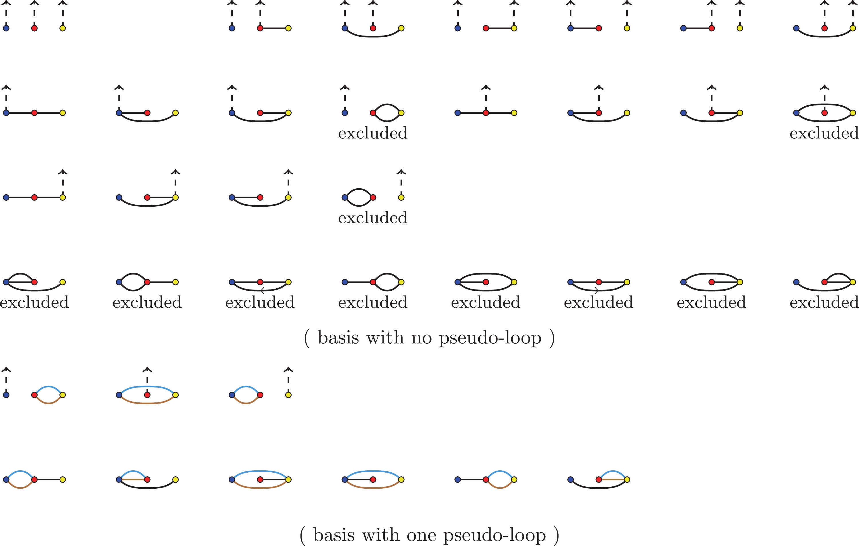
Figure 3. (color online) Quiver representation of gauge invariant basis for
$ A^{{ \rm{EYM}}}_{n,3} $ . For simplicity,$ h_1,h_2 $ , and$ h_3 $ are denoted as blue, red, and yellow dots, respectively. Arrows always flow from the starting points of the solid line toward pseudo-loops or the ending points of the dashed line, so they are omitted unless they cause confusion. The ending point of the dashed line is$ K_{a_i} $ depending on the$ h_i $ it connects, and$ 2\leqslant a_1,a_2,a_3 \leqslant n-1 $ . Quivers with real loops are excluded.$ {\cal C}[{\mathsf{F}}_{h_1}^{a_1}{\mathsf{F}}_{h_2}^{a_2}{\mathsf{F}}_{h_3}^{a_3}] = \left\{\begin{array}{*{20}{l}} A^{{\rm{YM}}}_{n+3}(1,2,\ldots,a_{\sigma_1},h_{\sigma_1},\ldots,a_{\sigma_2},h_{\sigma_2},\ldots,a_{\sigma_3},h_{\sigma_3},\ldots,n)\; \; ,& a_{\sigma_1}<a_{\sigma_2}<a_{\sigma_3} \\ \displaystyle\sum\nolimits_{\rho\{\sigma_2,\sigma_3\}\in S_2}A^{{\rm{YM}}}_{n+3}(1,2,\ldots,a_{\sigma_1},h_{\sigma_1},\ldots,a_{\sigma_2},h_{\rho_2},h_{\rho_3},a_{\sigma_2}+1,\ldots,n)\; \; ,& a_{\sigma_1}<a_{\sigma_2} = a_{\sigma_3} \\ \displaystyle\sum\nolimits_{\rho\{\sigma_1,\sigma_2\}\in S_2}A^{{\rm{YM}}}_{n+3}(1,2,\ldots,a_{\sigma_1},h_{\rho_1},h_{\rho_2},a_{\sigma_1}+1,\ldots,a_{\sigma_3},h_{\sigma_3},\ldots,n)\; \; ,& a_{\sigma_1} = a_{\sigma_2}<a_{\sigma_3} \\ \displaystyle\sum\nolimits_{\rho\{\sigma_1,\sigma_2,\sigma_3\}\in S_3}A^{{\rm{YM}}}_{n+3}(1,2,\ldots,a_{\sigma_1},h_{\rho_1},h_{\rho_2},h_{\rho_3},a_{\sigma_1}+1,\ldots,n)\; \; ,& a_{\sigma_1} = a_{\sigma_2} = a_{\sigma_3} \end{array} \right.\; ,\; \; \; $

where
$ \rho\{\sigma_1,\cdots,\sigma_m\} $ is a permutation of$ \{\sigma_1,\cdots,\sigma_m\} $ , and the summation is over all elements of$ S_m $ . Applying$ {\cal T}_{h_{\beta'_1}h_{\beta_1}n}{\cal T}_{a_{\gamma_1}h_{\gamma_1}(a_{\gamma_1}+1)}{\cal T}_{a_{\gamma_2}h_{\gamma_2}(a_{\gamma_2}+1)} $ to$ A^{{ \rm{EYM}}}_{n,3} $ , we get$ {\cal C}[{\mathsf{F}}_{h_{\beta_1}}^{h_{\beta'_1}}{\mathsf{F}}_{h_{\gamma_1}}^{a_{\gamma_1}}{\mathsf{F}}_{h_{\gamma_2}}^{a_{\gamma_2}}]\\ = \left\{\begin{array}{*{20}{l}} \displaystyle\sum\nolimits_{\shuffle}A^{{\rm{YM}}}_{n+3}(1,2,\ldots,a_{\gamma_1},h_{\gamma_1},\{ a_{\gamma_1}+1,\ldots,a_{\gamma_2},h_{\gamma_2},\ldots,n-1\}\shuffle \{h_{\beta_1}\},n)\; \; ,& a_{\gamma_1}<a_{\gamma_2}\; ,\; \beta'_1 = \gamma_1 \\ \displaystyle\sum\nolimits_{\shuffle}A^{{\rm{YM}}}_{n+3}(1,2,\ldots,a_{\gamma_1},h_{\gamma_1},\ldots,a_{\gamma_2},h_{\gamma_2},\{a_{\gamma_2}+1,\ldots,n-1\}\shuffle \{h_{\beta_1}\},n)\; \; ,& a_{\gamma_1}<a_{\gamma_2}\; ,\; \beta'_1 = \gamma_2 \\ \displaystyle\sum\nolimits_{\shuffle}A^{{\rm{YM}}}_{n+3}(1,2,\ldots,a_{\gamma_1},h_{\gamma_1},\{h_{\gamma_2},a_{\gamma_1}+1,\ldots,n-1\}\shuffle \{h_{\beta_1}\},n)\\ \quad +\displaystyle\sum\nolimits_{\shuffle}A^{{\rm{YM}}}_{n+3}(1,2,\ldots,a_{\gamma_1},h_{\gamma_2},h_{\gamma_1},\{a_{\gamma_1}+1,\ldots,n-1\}\shuffle \{h_{\beta_1}\},n)\; \; ,& a_{\gamma_1} = a_{\gamma_2}\; ,\; \beta'_1 = \gamma_1 \end{array} \right.\; ,\; \; \; $

where
$ \{\beta_1\}\cup \{\gamma_1,\gamma_2\} $ is a splitting of$ \{1,2,3\} $ . Applying$ {\cal T}_{h_{\beta'_1}h_{\beta_1}n}{\cal T}_{h_{\beta'_2}h_{\beta_2}n}{\cal T}_{a_{\gamma_1}h_{\gamma_1}(a_{\gamma_1}+1)} $ to$ A^{{ \rm{EYM}}}_{n,3} $ , we get$ {\cal C}[{\mathsf{F}}_{h_{\beta_1}}^{h_{\beta'_1}}{\mathsf{F}}_{h_{\beta_2}}^{h_{\beta'_2}}{\mathsf{F}}_{h_{\gamma_1}}^{a_{\gamma_1}}] = \left\{\begin{array}{*{20}{l}} \displaystyle\sum\nolimits_{\shuffle} A^{{\rm{YM}}}_{n+3}(1,2\ldots,a_{\gamma_1},h_{\gamma_1},\{a_{\gamma_1}+1,\ldots,n-1\}\shuffle\{h_{\beta_2},h_{\beta_1}\},n)\; \; ,& \beta'_1 = \beta_2\; ,\; \beta'_2 = \gamma_1\\ \displaystyle\sum\nolimits_{\shuffle}A^{{\rm{YM}}}_{n+3}(1,2\ldots,a_{\gamma_1},h_{\gamma_1},\{a_{\gamma_1}+1,\ldots,n-1\}\shuffle\{h_{\beta_2}\}\shuffle\{h_{\beta_1}\},n)\; \; ,& \beta'_1 = \gamma_1\; ,\; \beta'_2 = \gamma_1 \end{array}\right.\; ,\; \; \; $

with
$ \{\beta_1,\beta_2\}\cup \{\gamma_1\} = \{1,2,3\} $ . As mentioned, after summing over all the results produced in Step-0, we get a compact expression,$\tag{5.13} \begin{aligned} {[{\rm{Step}}\; 0]} = \sum\limits_{\shuffle} \frac{k_1\cdot f_{h_1}\cdot X_{h_1}}{k_1\cdot k_{h_1}}\frac{k_1\cdot f_{h_2}\cdot X_{h_2}}{k_1\cdot k_{h_2}} \frac{k_1\cdot f_{h_3}\cdot X_{h_3}}{k_1\cdot k_{h_3}}A^{{\rm{YM}}}_{n+3}(1,2,\{3,\ldots,n-1\}\shuffle \{h_1\}\shuffle \{h_2\}\shuffle\{h_3\},n)\; .\; \; \; \end{aligned} $

Recalling the compact expression (5.12) for the EYM amplitude with two gravitons, we confirm that is it always possible for the total contribution of Step-0 to be written in a compact form.
Then, we proceed to Step-1 and compute the expansion coefficients for vectors with one pseudo-loop. After substituting the solutions in Step-0 back into the expansion equation, we get
$\tag{5.14}\begin{aligned}[b] A^{{ \rm{EYM}}}_{n,3}-[{{\rm{Step}}\; 0}] =& \sum\limits_{\textstyle{a_{\gamma_1} = 2\atop \{\alpha_1,\alpha_2,\gamma_1\}}}^{n-1} {\cal C}[{\mathsf{F}}_{h_{\alpha_1}h_{\alpha_2}}{\mathsf{F}}_{h_{\gamma_1}}^{a_{\gamma_1}}] {\mathsf{F}}_{h_{\alpha_1}h_{\alpha_2}}{\mathsf{F}}_{h_{\gamma_1}}^{a_{\gamma_1}} \\&+\sum\limits_{\textstyle{\{\alpha_1,\alpha_2,\beta_1\}\atop \beta'_1\neq \beta_1}} {\cal C}[{\mathsf{F}}_{h_{\alpha_1}h_{\alpha_2}}{\mathsf{F}}_{h_{\beta_1}}^{h_{\beta'_1}}] {\mathsf{F}}_{h_{\alpha_1}h_{\alpha_2}}{\mathsf{F}}_{h_{\beta_1}}^{h_{\beta'_1}}\; ,\end{aligned} $

where the first summation runs over all possible splittings
$ \{\alpha_1,\alpha_2,\gamma_1\} $ of$ \{1,2,3\} $ , while the second summation runs over not only all splittings$ \{\alpha_1,\alpha_2,\beta_1\} $ but also all possible values of$ \beta'_1 $ . Terms in the first summation correspond to the first three quivers with one pseudo-loop in Fig. 3, while terms in the second summation correspond to the remaining six quivers. As mentioned, for a fixed value of p, we should start from terms with larger r, i.e., terms in the first summation. As argued in the previous section, when applying a defined differential operator, only the corresponding vector survives, and all others vanish. This means there are no mixing contributions between different pseudo-loops of the first type. For example, applying the differential operator$ {\cal T}_{h_3h_2n}{\cal T}_{1h_32} {\cal T}_{a_1h_1(a_1+1)} $ to equation (5.14), the only surviving vector with one pseudo-loop is$ {\mathsf{F}}_{h_2h_3}{\mathsf{F}}_{h_1}^{a_1} $ . However, vectors with no pseudo-loops would contribute, and from our previous general argument, we can determine the non-vanishing vectors to be$ {\mathsf{F}}_{h_2}^{h_3}{\mathsf{F}}^{K_a}_{h_3}{\mathsf{F}}_{h_1}^{a_1} $ and$ {\mathsf{F}}_{h_2}^{h_3}{\mathsf{F}}^{h_1}_{h_3}{\mathsf{F}}_{h_1}^{a_1} $ . Hence, we have$\tag{5.15} \begin{aligned}[b] {\cal C}[{\mathsf{F}}_{h_2h_3}{\mathsf{F}}_{h_1}^{a_1}] =& \Big(\; (k_1\cdot k_{h_3})({\cal T}_{h_3h_2n}{\cal T}_{1h_32}{\cal T}_{a_1h_1(a_1+1)}\; A^{{ \rm{EYM}}}_{n,3})\; \Big)\\ &+\Big(\; \sum\limits_{a_3 = 2}^{n-1}(k_{h_3}\cdot X_{h_3}){\cal C}[{\mathsf{F}}_{h_2}^{h_3}{\mathsf{F}}_{h_1}^{a_1}{\mathsf{F}}_{h_3}^{a_3}]\; \Big) \\&+\Big(\; (k_{h_3}\cdot k_{h_1}){\cal C}[{\mathsf{F}}_{h_2}^{h_3}{\mathsf{F}}_{h_3}^{h_1}{\mathsf{F}}_{h_1}^{a_1}]\; \Big)\; ,\; \; \; \end{aligned} $

where the relation (4.16) has been used. Working this out explicitly, we have
$\tag{5.16} \begin{aligned}[b] {\cal C}[{\mathsf{F}}_{h_2h_3}{\mathsf{F}}_{h_1}^{a_1}]=& (k_1\cdot k_{h_3}) A(1, h_3, \{h_2\} \shuffle\{2,...,a_1, h_1, a_1+1,...,n-1\}, n) \\&+(k_{h_3}\cdot X_{h_3}) A(1, 2, \{3,...,a_1, h_1, a_1+1,...,n-1\}\shuffle\{h_3, h_2\},n) \\ & + (k_{h_3}\cdot k_{h_1}) A(1, 2,...,a_1,h_1, \{h_3, h_2\}\shuffle\{a_1+1,...,n-1\}, n)\; .\end{aligned} $

Terms in the first and second lines are similar to those given in (5.9); hence, we can use the result (5.11) here and immediately work out the summation as
$\tag{5.17} \begin{aligned}[b] \sum\limits_{a_1 = 2}^{n-1} {\cal C}[{\mathsf{F}}_{h_2h_3}{\mathsf{F}}_{h_1}^{a_1}]{\mathsf{F}}_{h_2h_3}{\mathsf{F}}_{h_1}^{a_1} =& {\mathsf{F}}_{h_2h_3}{ (k_1\cdot f_{h_1}\cdot Y_{h_1})(k_{h_3}\cdot k_{h_1})\over(k_1\cdot k_{h_1})} A^{{\rm{YM}}}_{n+2}(1, 2,\{h_1, h_3, h_2\}\shuffle\{3,...,n-1\}, n) + \sum\limits_{\{\sigma_1,\sigma_2\}\in S_2(h_2, h_3)} \\ & \times{\mathsf{F}}_{h_2h_3}{ (k_1\cdot f_{h_1}\cdot Y_{h_1})\over(k_1\cdot k_{h_1})}\frac{(k_{h_{\sigma_1}}\cdot X_{h_{\sigma_1}}-k_1\cdot k_{h_{\sigma_1}})(k_{h_{\sigma_2}}\cdot X_{h_{\sigma_2}})}{{\cal K}_{1h_3h_2}} \\&\times A^{{\rm{YM}}}_{n+2}(1,2,\{3,\ldots,n-1\}\shuffle\{h_1\}\shuffle \{h_{\sigma_1},h_{\sigma_2}\},n)\; .\; \; \; \end{aligned} $

The other two terms with
$ r = 1 $ can be obtained by permutation of the above result.We now proceed to the vectors with
$ p = 1,r = 0 $ . As discussed, a defined differential operator (4.35) would possibly mix contributions of many vectors with one pseudo-loop, and in general, we should solve an algebraic system of linear equations to compute all of them. However, in the current simple example, we can intentionally choose a differential operator to avoid the mixing of vectors. For instance, to compute the coefficient of vector$ {\mathsf{F}}_{h_2h_3}{\mathsf{F}}_{h_1}^{h_2} $ we should choose the differential operator$ {\cal T}_{h_3h_2n}{\cal T}_{1h_32}{\cal T}_{h_2h_1n} $ . If instead we choose the other differential operator$ {\cal T}_{h_2h_3n}{\cal T}_{1h_2 2}{\cal T}_{h_2h_1n} $ , both vectors$ {\mathsf{F}}_{h_1h_2}{\mathsf{F}}_{h_3}^{h_2} $ and$ {\mathsf{F}}_{h_2h_3}{\mathsf{F}}_{h_1}^{h_2} $ would be non-vanishing, and their contributions will mix together. Hence, we apply$ {\cal T}_{h_3h_2n}{\cal T}_{1h_32}{\cal T}_{h_2h_1n} $ to equation (5.14) and compute the coefficient as follows:$\tag{5.18} \begin{aligned}[b] {\cal C}[{\mathsf{F}}_{h_2h_3}{\mathsf{F}}_{h_1}^{h_2}] = &\Big(\; (k_1\cdot k_{h_3})({\cal T}_{h_2h_1n}{\cal T}_{h_3h_2n}{\cal T}_{1h_32}\; A^{{ \rm{EYM}}}_{n,3})\; \Big)\\& +\Big(\; \sum\limits_{a_3 = 2}^{n-1}(k_{h_3}\cdot X_{h_3}){\cal C}[{\mathsf{F}}_{h_1}^{h_2}{\mathsf{F}}_{h_2}^{h_3}{\mathsf{F}}_{h_3}^{a_3}]\; \Big) \\ =& (k_1\cdot k_{h_3}) A^{{\rm{YM}}}_{n+3}(1, \{h_3, h_2, h_1\}\shuffle\{2,...,n-1\}_R, n)\\&+ (k_{h_3}\cdot X_{h_3}) A^{{\rm{YM}}}_{n+3}(1, 2,\{h_3, h_2, h_1\}\\& \shuffle\{3,...,n-1\}, n)\; .\; \; \; \end{aligned} $

The Yang-Mills amplitudes in the second term are already in the BCJ basis, with legs
$ 1,2,n $ fixed, while those in the first term should be rewritten to the BCJ basis by applying the BCJ relations. Similar computations can be inferred from (5.3) and (5.18); consequently, all coefficients of vectors with one pseudo-loop can be computed. Summing up the above results, we get the complete expansion of$ A^{{ \rm{EYM}}}_{n,3} $ , which is consistent with the results given in [33]. -
The EYM amplitude
$ A^{{ \rm{EYM}}}_{n,4}(1,\ldots,n;h_1,h_2,h_3,h_4) $ lives in the gauge invariant vector space$ {\cal W}_{n+4,4} $ , and it can be expanded as a linear combination of$ \dim{\cal W}_{n+4,4} = (n+1)^4+$ $6(n+1)^2+3 $ vectors. All vectors in the gauge invariant basis and their quivers are shown in Fig. 4. Among them, there are in total$ 6\times (n-2)^2+44(n-2)+87 $ vectors with real loops, which should be excluded. We can compute the expansion coefficients of the remaining vectors using the algorithm. Again, in Step-0, we compute the coefficients of vectors with no pseudo-loops using equation (4.34). We shall not write down the explicit coefficient for each basis; rather, we present their summation in a compact expression as ㉖,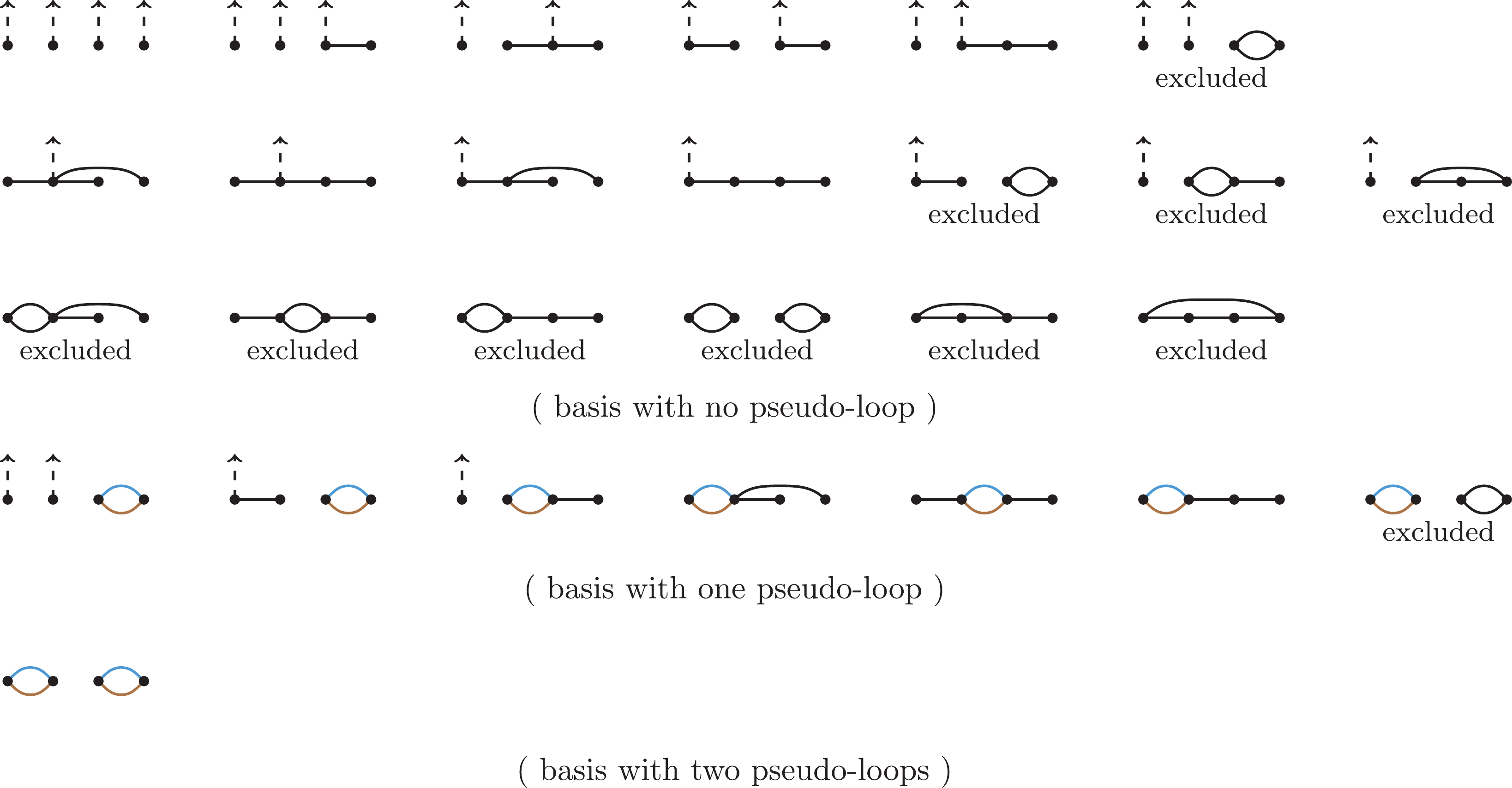
Figure 4. (color online) Quiver representation of gauge invariant basis for
$ A^{{ \rm{EYM}}}_{n,4} $ . For presentation purposes, we only show quivers of distinct topologies, and a graph here denotes several graphs with black dots specifying any possible independent label$ (h_1,h_2,h_3,h_4) $ . Arrows always flow from the starting point of the solid line toward pseudo-loops or the ending point of the dashed line, and they are omitted unless they cause confusion. The ending point of the dashed line is$ K_{a_i} $ depending on the$ h_i $ it connects to, and$ 2\leqslant a_1,a_2,a_3, a_4 \leqslant n-1 $ . Quiver graphs with real solid loops are excluded.$\tag{5.19}\begin{aligned}[b] [{{\rm{Step}}\; 0}] =& \sum\limits_{\shuffle} \left(\prod\limits_{i = 1}^{4}\frac{k_1\cdot f_{h_i}\cdot X_{h_i}}{k_1\cdot k_{h_i}}\right)A^{{\rm{YM}}}_{n+4}(1,2,\{3,\ldots,n-1\}\\& \shuffle \{h_1\}\shuffle \{h_2\}\shuffle\{h_3\}\shuffle\{h_4\},n)\; .\\[-15pt]\end{aligned} $

Then, let us proceed with Step-1, to compute the expansion coefficients of vectors with one pseudo-loop. As shown in Fig. 4, there are in total seven distinct topologies, and the last one should be excluded. For the other six topologies, according to rules (4.19), we assign each of them to a respective differential operator, and we represent differential operators in quiver representation as
where without ambiguity, we have ignored the dashed line
$ (h_a1) $ corresponding to$ (k_1k_{h_a}){\cal T}_{1h_a2} $ , which is always linked to the ending point of the cyan line. The first two quivers of differential operators are consistent with rules (4.18), and they are sufficient to distinguish the corresponding vectors uniquely. For the third and fourth quivers of differential operators, noting the choice of direction of the cyan line, we know that they are also able to determine the expansion coefficients without mixing contributions from other vectors with one pseudo-loop. However, the last two types of vectors do mix together under the defined differential operators. The sixth quiver of differential operators is able to distinguish the sixth type of vectors. However, with the fifth quiver of differential operators, contributions from the fifth type of vectors would be mixed up with those from the sixth type of vectors. Although we can disentangle all vectors by constructing linear combinations of differential operators as in equation (4.31), in the current simple example, we have an alternative way of solving equations. By first solving the coefficients of vectors of the sixth topology and then solving the vectors of the fifth topology, but with the former solutions as known inputs, we are able to compute all coefficients order by order. Furthermore, we wish to emphasize that the differential operators also pick up contributions from vectors with no pseudo-loops, and we should compute all coefficients of vectors with no pseudo-loops before computing those of vectors with one pseudo-loop.Let us analyze these six topologies one by one. For the first topology, the corresponding differential operator also picks up the following contributions in Step-0,
For instance, using the differential operator
$ (k_1\cdot k_{h_4}){\cal T}_{h_4h_3n}{\cal T}_{1h_42}{\cal T}_{a_1h_1(a_1+1)}{\cal T}_{a_2h_2(a_2+1)} $ , we can compute the coefficient of$ {\cal B}[{\mathsf{F}}_{h_3h_4}{\mathsf{F}}_{h_1}^{a_1}{\mathsf{F}}_{h_2}^{a_2}] $ as$ \begin{aligned}[b]{\cal C}[{\mathsf{F}}_{h_3h_4}{\mathsf{F}}_{h_1}^{a_1}{\mathsf{F}}_{h_2}^{a_2}] =& \Big(\; (k_1\cdot k_{h_4})({\cal T}_{h_4h_3n}{\cal T}_{1h_42}{\cal T}_{a_1h_1(a_1+1)}{\cal T}_{a_2h_2(a_2+1)}\; A^{{ \rm{EYM}}}_{n,4})\; \Big)\\ & +\Big(\; \sum\limits_{a_4 = 2}^{n-1}(k_{h_4}\cdot X_{h_4}){\cal C}[{\mathsf{F}}_{h_3}^{h_4}{\mathsf{F}}_{h_1}^{a_1}{\mathsf{F}}_{h_2}^{a_2}{\mathsf{F}}_{h_4}^{a_4}]\; \Big)+\Big(\; (k_{h_1}\cdot k_{h_4}){\cal C}[{\mathsf{F}}_{h_3}^{h_4}{\mathsf{F}}_{h_4}^{h_1}{\mathsf{F}}_{h_1}^{a_1}{\mathsf{F}}_{h_2}^{a_2}]+(k_{h_2}\cdot k_{h_4}){\cal C}[{\mathsf{F}}_{h_3}^{h_4}{\mathsf{F}}_{h_4}^{h_2}{\mathsf{F}}_{h_1}^{a_1}{\mathsf{F}}_{h_2}^{a_2}]\; \Big)\; .\; \; \; \end{aligned} $

Applying the differential operator on
$ A^{{ \rm{EYM}}}_{n,4} $ produces Yang-Mills amplitudes$ A^{{\rm{YM}}}_{n+4}(1,h_4,\{2,\ldots,a_1,h_1,\ldots,a_2,h_2,\ldots,n-1\}\shuffle \{h_3\},n)\; ,\; \; \; $

and using the BCJ relations, they can be rewritten into the BCJ basis.
For the second topology, the corresponding differential operator picks up the following contributions in Step-0,
For instance, using the differential operator
$ (k_1\cdot k_{h_4}){\cal T}_{h_4h_3n}{\cal T}_{1h_42}{\cal T}_{h_1h_2n}{\cal T}_{a_1h_1(a_1+1)} $ , we can compute the coefficient of$ {\cal B}[{\mathsf{F}}_{h_3h_4}{\mathsf{F}}_{h_2}^{h_1}{\mathsf{F}}_{h_1}^{a_1}] $ as$ \begin{aligned}[b]{\cal C}[{\mathsf{F}}_{h_3h_4}{\mathsf{F}}_{h_2}^{h_1}{\mathsf{F}}_{h_1}^{a_1}] =& \Big(\; (k_1\cdot k_{h_4})({\cal T}_{h_4h_3n}{\cal T}_{1h_42}{\cal T}_{h_1h_2n}{\cal T}_{a_1h_1(a_1+1)}\; A^{{ \rm{EYM}}}_{n,4})\; \Big)\\ &+\Big(\; \sum\limits_{a_4 = 2}^{n-1}(k_{h_4}\cdot X_{h_4}){\cal C}[{\mathsf{F}}_{h_2}^{h_1}{\mathsf{F}}_{h_3}^{h_4}{\mathsf{F}}_{h_1}^{a_1}{\mathsf{F}}_{h_4}^{a_4}]\; \Big)+\Big(\; (k_{h_1}\cdot k_{h_4}){\cal C}[{\mathsf{F}}_{h_2}^{h_1}{\mathsf{F}}_{h_3}^{h_4}{\mathsf{F}}_{h_4}^{h_1}{\mathsf{F}}_{h_1}^{a_1}]\; \Big)+\Big(\; (k_{h_2}\cdot k_{h_4}){\cal C}[{\mathsf{F}}_{h_2}^{h_1}{\mathsf{F}}_{h_3}^{h_4}{\mathsf{F}}_{h_4}^{h_2}{\mathsf{F}}_{h_1}^{a_1}]\; \Big)\; .\; \; \; \end{aligned} $

Applying the differential operator on
$ A^{{ \rm{EYM}}}_{n,4} $ produces Yang-Mills amplitudes$ A^{{\rm{YM}}}_{n+4}(1,h_4,\{\; 2,\ldots,a_1,h_1,\{a_1+1,\ldots,n-1\}\shuffle \{h_2\}\; \}\shuffle \{h_3\},n)\; .\; \; \; $

For the third topology, the corresponding differential operator picks up the following contributions in Step-0,
For instance, using the differential operator
$ (k_1\cdot k_{h_4}){\cal T}_{h_4h_3n}{\cal T}_{1h_42}{\cal T}_{h_3h_2n}{\cal T}_{a_1h_1(a_1+1)} $ , we can compute the coefficient of$ {\cal B}[{\mathsf{F}}_{h_3h_4}{\mathsf{F}}_{h_2}^{h_3}{\mathsf{F}}_{h_1}^{a_1}] $ as$\tag{5.20} \begin{aligned}[b] {\cal C}[{\mathsf{F}}_{h_3h_4}{\mathsf{F}}_{h_2}^{h_3}{\mathsf{F}}_{h_1}^{a_1}] =& \Big(\; (k_1\cdot k_{h_4})({\cal T}_{h_4h_3n}{\cal T}_{1h_42}{\cal T}_{h_3h_2n}{\cal T}_{a_1h_1(a_1+1)}\; A^{{ \rm{EYM}}}_{n,4})\; \Big)\\& +\Big(\; \sum\limits_{a_4 = 2}^{n-1}(k_{h_4}\cdot X_{h_4}){\cal C}[{\mathsf{F}}_{h_2}^{h_3}{\mathsf{F}}_{h_3}^{h_4}{\mathsf{F}}_{h_1}^{a_1}{\mathsf{F}}_{h_4}^{a_4}]\; \Big)+\Big(\; (k_{h_1}\cdot k_{h_4}){\cal C}[{\mathsf{F}}_{h_2}^{h_3}{\mathsf{F}}_{h_3}^{h_4}{\mathsf{F}}_{h_4}^{h_1}{\mathsf{F}}_{h_1}^{a_1}]\; \Big)\; .\; \; \; \end{aligned} $

Applying the differential operator on
$ A^{{ \rm{EYM}}}_{n,4} $ produces Yang-Mills amplitudes$ A^{{\rm{YM}}}_{n+4}(1,h_4,\{2,\ldots,a_1,h_1,\ldots,n-1\}\shuffle \{h_3,h_2\},n)\; .\; \; \; $

For the fourth topology, the corresponding differential operator picks up the following contributions in Step-0,
For instance, using the differential operator
$ (k_1\cdot k_{h_4}){\cal T}_{h_4h_3n}{\cal T}_{1h_42}{\cal T}_{h_3h_1n}{\cal T}_{h_3h_2n} $ , we can compute the coefficient of$ {\cal B}[{\mathsf{F}}_{h_3h_4}{\mathsf{F}}_{h_1}^{h_3}{\mathsf{F}}_{h_2}^{h_3}] $ as$\begin{aligned}[b] {\cal C}[{\mathsf{F}}_{h_3h_4}{\mathsf{F}}_{h_1}^{h_3}{\mathsf{F}}_{h_2}^{h_3}] =& \Big(\; (k_1\cdot k_{h_4})({\cal T}_{h_4h_3n}{\cal T}_{1h_42}{\cal T}_{h_3h_1n}{\cal T}_{h_3h_2n}\; A^{{ \rm{EYM}}}_{n,4})\; \Big)\\&+\Big(\; \sum\limits_{a_4 = 2}^{n-1}(k_{h_4}\cdot X_{h_4}){\cal C}[{\mathsf{F}}_{h_1}^{h_3}{\mathsf{F}}_{h_2}^{h_3}{\mathsf{F}}_{h_3}^{h_4}{\mathsf{F}}_{h_4}^{a_4}]\; \Big)\; .\end{aligned} $

Applying the differential operator on
$ A^{{ \rm{EYM}}}_{n,4} $ produces Yang-Mills amplitudes$ \sum\limits_{\{\sigma_1,\sigma_2\}\in S_2}A^{{\rm{YM}}}_{n+4}(1,h_4,\{2,\ldots,n-1\}\shuffle \{h_3,h_{\sigma_1},h_{\sigma_2}\},n)\; .\; \; \; $

According to our discussion, we will consider the sixth topology before the fifth. The corresponding differential operator picks up the following contributions in Step-0,
For instance, using the differential operator
$ (k_1\cdot k_{h_4}){\cal T}_{h_4h_3n}{\cal T}_{1h_42}{\cal T}_{h_2h_1n}{\cal T}_{h_3h_2n} $ , we can compute the coefficient of$ {\cal B}[{\mathsf{F}}_{h_3h_4}{\mathsf{F}}_{h_1}^{h_2}{\mathsf{F}}_{h_2}^{h_3}] $ as$ \begin{aligned}[b] {\cal C}[{\mathsf{F}}_{h_3h_4}{\mathsf{F}}_{h_1}^{h_2}{\mathsf{F}}_{h_2}^{h_3}] = &\Big(\; (k_1\cdot k_{h_4})({\cal T}_{h_4h_3n}{\cal T}_{1h_42}{\cal T}_{h_2h_1n}{\cal T}_{h_3h_2n}\; A^{{ \rm{EYM}}}_{n,4})\; \Big)\\&+\Big(\; \sum\limits_{a_4 = 2}^{n-1}(k_{h_4}\cdot X_{h_4}){\cal C}[{\mathsf{F}}_{h_1}^{h_2}{\mathsf{F}}_{h_2}^{h_3}{\mathsf{F}}_{h_3}^{h_4}{\mathsf{F}}_{h_4}^{a_4}]\; \Big)\; .\end{aligned} $

Applying the differential operator on
$ A^{{ \rm{EYM}}}_{n,4} $ produces Yang-Mills amplitudes$ A^{{\rm{YM}}}_{n+4}(1,h_4,\{2,\ldots,n-1\}\shuffle \{h_3,h_2,h_1\},n)\; .\; \; \; $

Then, we come to the last portion. In addition to the contribution from the sixth topology, the differential operator corresponding to the fifth topology also picks up following contributions in Step-0,
Let us consider an example, with the differential operator
$ (k_1\cdot k_{h_4}){\cal T}_{h_4h_3n}{\cal T}_{1h_42}{\cal T}_{h_3h_1n}{\cal T}_{h_4h_2n} $ . We can use it to compute the coefficient of$ {\cal B}[{\mathsf{F}}_{h_3h_4}{\mathsf{F}}_{h_1}^{h_3}{\mathsf{F}}_{h_2}^{h_4}] $ as$\tag{5.21} \begin{aligned} {\cal C}[{\mathsf{F}}_{h_3h_4}{\mathsf{F}}_{h_1}^{h_3}{\mathsf{F}}_{h_2}^{h_4}] = & \Big(\; (k_1\cdot k_{h_4})({\cal T}_{h_4h_3n}{\cal T}_{1h_42}{\cal T}_{h_3h_1n}{\cal T}_{h_4h_2n}\; A^{{ \rm{EYM}}}_{n,4})\; \Big) \\& +\Big(\; \sum\limits_{a_4 = 2}^{n-1}(k_{h_4}\cdot X_{h_4}){\cal C}[{\mathsf{F}}_{h_1}^{h_3}{\mathsf{F}}_{h_2}^{h_4}{\mathsf{F}}_{h_3}^{h_4}{\mathsf{F}}_{h_4}^{a_4}]\; \Big) -{\cal C}[{\mathsf{F}}_{h_2h_4}F_{h_3}^{h_4}F_{h_1}^{h_3}]\; .\; \; \; \end{alinged} $

Applying the differential operator on
$ A^{{ \rm{EYM}}}_{n,4} $ produces Yang-Mills amplitudes$ A^{{\rm{YM}}}_{n+4}(1,h_4,\{2,\ldots,n-1\}\shuffle \{h_3,h_1\}\shuffle \{h_2\},n)\; .\; \; \; $

The computations above provide all of the expansion coefficients for the gauge invariant basis with one pseudo-loop based on the solutions in Step-0 and the BCJ relations.
Let us proceed to Step-2, where there are only three different vectors:
$ {\cal B}[{\mathsf{F}}_{h_1h_2}{\mathsf{F}}_{h_3h_4}] $ ,$ {\cal B}[{\mathsf{F}}_{h_1h_3}{\mathsf{F}}_{h_2h_4}] $ , and$ {\cal B}[{\mathsf{F}}_{h_1h_4}{\mathsf{F}}_{h_2h_3}] $ . According to the rule, we define differential operators for them respectively as$\tag{5.22} {\cal T}_{h_2h_1n}{\cal T}_{h_4h_3n}{\cal T}_{1h_22}{\cal T}_{1h_42}\; \; \; ,\quad {\cal T}_{h_3h_1n}{\cal T}_{h_4h_2n}{\cal T}_{1h_32}{\cal T}_{1h_44}\; \; \; ,\quad {\cal T}_{h_4h_1n}{\cal T}_{h_3h_2n}{\cal T}_{1h_32}{\cal T}_{1h_42}\; .$

It can be checked directly that each differential operator picks up only one vector with two pseudo-loops, while it also picks up the respective contributions from Step-0 and Step-1,
For instance, using the differential operator
$ {\cal T}_{h_2h_1n}{\cal T}_{h_4h_3n}{\cal T}_{1h_22}{\cal T}_{1h_42} $ we can compute the coefficient of$ {\cal B}[{\mathsf{F}}_{h_1h_2}{\mathsf{F}}_{h_3h_4}] $ as$ {\cal C}[{\mathsf{F}}_{h_1h_2}{\mathsf{F}}_{h_3h_4}] = \Big((k_1\cdot k_{h_2})(k_1\cdot k_{h_4})({\cal T}_{h_2h_1n}{\cal T}_{h_4h_3n}{\cal T}_{1h_22}{\cal T}_{1h_42}\; A^{{ \rm{EYM}}}_{n,4})\Big)+\Big([{{\rm{Step}}-0}]+[{{\rm{Step}}-1}]\Big)\Big|_{{\mathsf{F}}_{h_1h_2}{\mathsf{F}}_{h_3h_4}}\; ,\; \; \; $

where
$\tag{5.23} \begin{aligned}[b] [{{\rm{Step}}-0}]\Big|_{{\mathsf{F}}_{h_1h_2}{\mathsf{F}}_{h_3h_4}} =& \Big(\sum\limits_{a_2 = 2}^{n-1}\sum\limits_{a_4 = 2}^{n-1} (k_{h_2}\cdot X_{h_2})(k_{h_4}\cdot X_{h_4}){\cal C}[{\mathsf{F}}_{h_1}^{h_2}{\mathsf{F}}_{h_3}^{h_4}{\mathsf{F}}_{h_2}^{a_2}{\mathsf{F}}_{h_4}^{a_4}]\Big)\\&+\Big(\sum\limits_{a_2 = 2}^{n-1} \sum\limits_{i = 1,2} (k_{h_2}\cdot X_{h_2})(k_{h_4}\cdot k_{h_i}){\cal C}[{\mathsf{F}}_{h_1}^{h_2}{\mathsf{F}}_{h_3}^{h_4}{\mathsf{F}}_{h_4}^{h_i}{\mathsf{F}}_{h_2}^{a_2}]\Big)+\Big(\sum\limits_{a_4 = 2}^{n-1} \sum\limits_{i = 3,4} (k_{h_4}\cdot X_{h_4})(k_{h_2}\cdot k_{h_i}){\cal C}[{\mathsf{F}}_{h_1}^{h_2}{\mathsf{F}}_{h_2}^{h_i}{\mathsf{F}}_{h_3}^{h_4}{\mathsf{F}}_{h_4}^{a_4}]\Big)\; ,\; \; \; \end{aligned} $

is the contribution from expansion in Step-0, and
$ \tag{5.24}\begin{aligned}[b] [{{\rm{Step}}-1}]\Big|_{{\mathsf{F}}_{h_1h_2}{\mathsf{F}}_{h_3h_4}} =& \Big(\sum\limits_{a_2 = 2}^{n-1}(k_{h_2}\cdot X_{h_2}){\cal C}[{\mathsf{F}}_{h_3h_4}{\mathsf{F}}_{h_1}^{h_2}{\mathsf{F}}_{h_2}^{a_2}]+\sum\limits_{i = 3,4}(k_{h_2}\cdot k_{h_i}){\cal C}[{\mathsf{F}}_{h_3h_4}{\mathsf{F}}_{h_1}^{h_2}{\mathsf{F}}_{h_2}^{h_i}]\Big)\\ & +\Big(\sum\limits_{a_4 = 2}^{n-1}(k_{h_4}\cdot X_{h_4}){\cal C}[{\mathsf{F}}_{h_1h_2}{\mathsf{F}}_{h_3}^{h_4}{\mathsf{F}}_{h_4}^{a_4}]+\sum\limits_{i = 1,2}(k_{h_4}\cdot k_{h_i}){\cal C}[{\mathsf{F}}_{h_1h_2}{\mathsf{F}}_{h_3}^{h_4}{\mathsf{F}}_{h_4}^{h_i}]\Big)+\Big((k_{h_2}\cdot k_{h_4}){\cal C}[{\mathsf{F}}_{h_2h_4}{\mathsf{F}}_{h_1}^{h_2}{\mathsf{F}}_{h_3}^{h_4}]\Big)\; ,\; \; \; \end{aligned} $

is the contribution from expansion in Step-1. Applying the differential operator on
$ A^{{ \rm{EYM}}}_{n,4} $ produces Yang-Mills amplitudes$\tag{5.25} \begin{aligned}[b]& \sum_{\{\sigma_2,\sigma_4\}\in S_2}A^{{\rm{YM}}}_{n+4}(1,h_{\sigma_2},h_{\sigma_4},\{2,\ldots,n-1\}\shuffle\{h_1\}\shuffle \{h_3\},n)\\ &\quad +A^{{\rm{YM}}}_{n+4}(1,h_2,h_1,h_4,\{2,\ldots,n-1\}\shuffle \{h_3\},n)+A^{{\rm{YM}}}_{n+4}(1,h_4,h_3,h_2,\{2,\ldots,n-1\}\shuffle \{h_1\},n)\;. \end{aligned} $

Then, using the BCJ relations for
$ A^{{\rm{YM}}}(1,\alpha_1,2,\ldots,n) $ ,$ A^{{\rm{YM}}}(1,\alpha_1,\alpha_2,2,\ldots,n) $ ,$ A^{{\rm{YM}}}(1,\alpha_1,\alpha_2,\alpha_3,2,\ldots,n) $ , and$ A^{{\rm{YM}}}(1,\alpha_1,\alpha_2,\alpha_3,\alpha_4,2,\ldots,n) $ we can rewrite all of the Yang-Mills amplitudes into the BCJ basis with legs$ 1,2,n $ fixed. Collecting the above results, we obtain the required EYM amplitude expansion. Because the final result is complicated, we do not present the explicit expression for$ A^{{ \rm{EYM}}}_{n,4}(1,\cdots,n;h_1,h_2,h_3,h_4) $ . However, we have numerically checked the algorithm up to$ A^{{ \rm{EYM}}}_{6,4} $ and found agreement with CHY formalism. -
There are already quite a few well-formulated results for expansion of EYM amplitudes to Yang-Mills amplitudes in the KK basis; however, a compact expression or even a recursive formula for expansion to Yang-Mills amplitudes in the BCJ basis is still required. The latter expansion is generally much more complicated than conventionally expected. In the KK basis, the expansion coefficients of Yang-Mills amplitudes are only polynomials of polarizations and momenta, and they are constrained to explicit compact expressions by gauge invariance. In the BCJ basis, the expansion coefficients of Yang-Mills amplitudes are instead rational functions, whose explicit form is much more difficult to determine. This is why we considered using differential operators to determine expansion coefficients in [33].
This paper is motivated by the problem of expanding EYM amplitudes to Yang-Mills amplitudes in the BCJ basis using differential operators. We have implemented an algorithm to systematically perform the expansion and compute the expansion coefficients. However, the EYM amplitude is not directly expanded to the BCJ basis but rather to a basis in gauge invariant vector space, as schematically shown in equation (4.1). After determining the expansion coefficients, we transform Yang-Mills amplitudes to the BCJ basis using the BCJ relations. Expanding EYM amplitude in a manifest gauge invariant form for both the expansion basis and its coefficients is a very interesting point of view, and differential operators can be naturally introduced into the problem. This contributes to our major results.
The first major part of this paper is devoted to the construction of a gauge invariant basis and the corresponding differential operators. A systematic algorithm is built upon the properties of applying differential operators on different bases. To construct a complete set of manifestly gauge invariant polynomials as the expansion basis, we start from the most general vector space
$ {\cal V}_{n,m} $ with$ m\leq n $ , where all possible polynomials of Lorentz contractions among polarizations and momenta live in this space, obeying some additional conditions. Then, we define a linear mapping$ {\cal G}_i $ , which is a realization of gauge invariant condition for polarization. By taking the interaction of kernels of all possible$ {\cal G}_i $ , we construct the gauge invariant sub-space$ {\cal W}_{n,m} $ from$ {\cal V}_{n,m} $ , which is the vector space containing all gauge invariant polynomials. This is also the space where the expansion basis of EYM amplitude lives. We present the formula for computing the dimension of$ {\cal W}_{n,m} $ , which indicates the number of gauge invariant vectors to which an EYM amplitude would be expanded. We also find that the gauge invariant vectors can be realized by linear combinations of multiplications of fundamental f-terms. These results finally help us construct a linearly independent and complete basis combinatorially for EYM amplitude expansion.After clarifying the structure of the gauge invariant expansion basis, we further construct differential operators from multiplication of insertion operators. The differential operators are constructed such that when applying a differential operator on an expression, only one particular vector in the gauge invariant basis is non-vanishing, while all others vanish. To do so, we start by analyzing the structures of the gauge invariant basis and finding the quiver representation for them. With the help of the quiver representation, we summarize all possible components appearing in the gauge invariant vectors and provide mapping rules for writing a differential operator directly from a gauge invariant vector, as multiplication of three basic types of insertion operators. Based on the above results, an algorithm for expansion of EYM amplitudes is implemented, with the idea of solving algebraic systems of linear equations order by order. To demonstrate the algorithm, we present the expansions of EYM amplitudes with up to four gravitons in the language of the gauge invariant basis, which are all consistent with CHY formalism numerically.
Although the algorithm for expanding the tree-level single-trace EYM amplitude to the Yang-Mills amplitudes in the BCJ basis has been thoroughly provided in this paper, it still inspires further work for the future. First, the expansion coefficients of the BCJ basis demand an explicit and possibly compact formulation. It is a rather difficult problem, but we have found some clues in results (5.9) and (5.18) already and hope they can help to determine the general picture. Second, in this paper, we only deal with single-trace EYM amplitudes, while discussions can be generalized to multi-trace EYM amplitudes using the trace operator
$ {\cal T}_{\epsilon_i\epsilon_j} $ . We think this generalization should be straightforward.Third, in this paper, we focus on EYM amplitudes, so the parameters of vector space
$ {\cal V}_{n,m} $ are constrained to$ m<n $ . However, the case$ m = n $ is also very interesting in physics because Yang-Mills amplitudes live in this space. Another interesting example is the deformed Yang-Mills theory with the$ F^3 $ term [48, 49]. Although the dimension of$ {\cal W}_{n,m} $ still holds for$ m = n $ , the explicit form of vectors in the gauge invariant basis should be reconsidered because we are not able to trivially exclude momentum$ k_n $ in all expressions by momentum conservation. Furthermore, for the Yang-Mills amplitude, an additional constraint should be applied to the vector space, i.e., there should be at least one$ (\epsilon\cdot \epsilon) $ contraction, and we can denote the vector space by$ \widetilde{W}_{n,m} $ . The new vector space$ \widetilde{W}_{n,m} $ can help us to understand the implication of gauge invariance in Yang-Mills amplitudes more deeply, along the lines of previous studies in [8, 37, 38]. It is also a curious problem to write Yang-Mills amplitudes in a manifestly gauge invariant form. Perhaps, it can also help us to understand more about the Pfaffian in the integrand of the CHY formula and provide a new point of view for the BCJ relations.We are grateful to Kang Zhou, ZhongJie Huang, and Yiwen Lin for discussions about this work. Xiao-Di Li would like to thank Yi-Jian Du for his enlightening discussions and kind hospitality at Wuhan University.
-
Proof of proposition 1: We wish to prove the following splitting formula of linear maps
$ {\cal G}_1,{\cal G}_2 $ ,$\tag{A1} {\rm{Ker}}\; {\cal G}_1+{\rm{Ker}}\; {\cal G}_2 = {\rm{Ker}}\; {\cal G}_1{\cal G}_2\; .\; \; \; $

To do so, it is sufficient to show
$\tag{A2} {\rm{Ker}}\; {\cal G}_1+{\rm{Ker}}\; {\cal G}_2 \subseteq {\rm{Ker}}\; {\cal G}_1{\cal G}_2\; \; \; {\rm{and}}\; \; \; {\rm{Ker}}\; {\cal G}_1+{\rm{Ker}}\; {\cal G}_2 \supseteq {\rm{Ker}}\; {\cal G}_1{\cal G}_2\; .\; \; \; $

The proof of
$ {\rm{Ker}}\; {\cal G}_1+{\rm{Ker}}\; {\cal G}_2 \subseteq {\rm{Ker}}\; {\cal G}_1{\cal G}_2 $ is trivial. Each$ v\in {\rm{Ker}}\; {\cal G}_1+{\rm{Ker}}\; {\cal G}_2 $ can always be written as$ v = v_1+v_2\; \; \; ,\; \; \; v_i\in {\rm{Ker}}\; {\cal G}_i\; \; {\rm{and}}\; \; \; {\cal G}_iv_i = 0\; .\; \; \; $

Thus, the action of
$ {\cal G}_1{\cal G}_2 $ on v is$\tag{A3} {\cal G}_1{\cal G}_2 v = {\cal G}_1{\cal G}_2 v_1+{\cal G}_1{\cal G}_2 v_2 = {\cal G}_2({\cal G}_1 v_1)+{\cal G}_1({\cal G}_2 v_2) = 0\; ,\; \; \; $

where we have used the commutative of
$ {\cal G}_i $ , i.e.,$ {\cal G}_1{\cal G}_2 = {\cal G}_2{\cal G}_1 $ . Hence,$ v\in {\rm{Ker}}\; {\cal G}_1{\cal G}_2 $ , and consequently,$ {\rm{Ker}}\; {\cal G}_1+{\rm{Ker}}\; {\cal G}_2 \subseteq {\rm{Ker}}\; {\cal G}_1{\cal G}_2 $ .The proof of
$ {\rm{Ker}}\; {\cal G}_1+{\rm{Ker}}\; {\cal G}_2 \supseteq {\rm{Ker}}\; {\cal G}_1{\cal G}_2 $ is not easy, so we will prove it by induction. Let us start from the vector space$ {\cal V}_{n,2} $ , i.e., containing only two polarizations$ \epsilon_1,\epsilon_2 $ . A polynomial$ {\mathfrak{h}}_{n,2} $ in$ {\cal V}_{n,2} $ can be written as$\tag{A4} {\mathfrak{h}}_{n,2} = \alpha_1(\epsilon_1\cdot \epsilon_2)+\sum\limits_{i,j = 1}^{n-1}\alpha_{2}^{ij}(\epsilon_1\cdot k_i)(\epsilon_2\cdot k_j)\; ,\; \; \; $

where momentum conservation has been used to eliminate the appearance of
$ k_n $ . For$ {\mathfrak{h}}_{n,2}\in\; {\rm{Ker}}\; {\cal G}_1{\cal G}_2 $ , by imposing$ {\cal G}_1{\cal G}_2{\mathfrak{h}}_{n,2} = 0 $ , we get$\tag{A5} {\cal G}_1{\cal G}_2{\mathfrak{h}}_{n,2} = {\mathfrak{h}}_{n,2}|_{{\epsilon_1\to k_1 \atop \epsilon_2\to k_2}} = \alpha_1(k_1\cdot k_2)+\sum\limits_{i,j = 1}^{n-1}\alpha_2^{ij}(k_1\cdot k_i)(k_2\cdot k_j) = 0\; .\; \; \; $

From the above equation, we can solve
$ \alpha_1 $ and substitute it back into$ {\mathfrak{h}}_{n,2} $ . After reorganization of terms, we get$\tag{A6} {\mathfrak{h}}_{n,2} = \sum\limits_{i,j = 1}^{n-1} \alpha_2^{ij} \frac{\epsilon_2\cdot f_1\cdot k_i}{k_1\cdot k_2}(k_2\cdot k_j)+\sum\limits_{i,j = 1}^{n-1} \alpha_2^{ij} \frac{k_1\cdot f_2\cdot k_j}{k_1\cdot k_2}(\epsilon_1\cdot k_i): = v_1+v_2\; .\; \; \; $

Because of the appearance of
$ f_i $ , it is easy to see that$ {\cal G}_i v_i = 0 $ . Hence,$ v_1\in {\rm{Ker}}\; {\cal G}_1 $ and$ v_2\in {\rm{Ker}}\; {\cal G}_2 $ . This shows that if$ {\mathfrak{h}}_{n,2}\in\; {\rm{Ker}}\; {\cal G}_1{\cal G}_2 $ , there is also$ {\mathfrak{h}}_{n,2}\in\; {\rm{Ker}}\; {\cal G}_1+{\rm{Ker}}\; {\cal G}_2 $ .Now, let us assume that for all vector spaces
$ {\cal V}_{n,s}, s<m $ , if a polynomial$ {\mathfrak{h}}_{n,s}\in {\rm{Ker}}\; {\cal G}_1{\cal G}_2 $ , then it can always be separated into two parts, one part belonging to$ {\rm{Ker}}\; {\cal G}_1 $ and the other belonging to$ {\rm{Ker}}\; {\cal G}_2 $ . A polynomial$ {\mathfrak{h}}_{n,m} $ in the vector space$ {\cal V}_{n,m} $ can be expanded to$\tag{A7} {\mathfrak{h}}_{n,m} = \sum\limits_{i = 1}^{m-1}(\epsilon_m\cdot \epsilon_i) T_{mi}+\sum\limits_{i = 1}^{m-1}(\epsilon_m\cdot k_i)(\epsilon_i\cdot T'_{mi})+\sum\limits_{i = m+1}^{n-1}(\epsilon_m\cdot k_i) T''_{mi}\; ,\; \; \; $

where
$ T_{mi}\in {\cal V}_{n,m-2} $ and$ \epsilon_i\cdot T'_{mi}\; ,\; T''_{mi}\in {\cal V}_{n,m-1} $ . For$ {\mathfrak{h}}_{n,m}\in {\rm{Ker}}\; {\cal G}_1{\cal G}_2 $ , by definition we have$\tag{A8} \begin{aligned}[b] 0 =& {\mathfrak{h}}_{n,m}|_{\epsilon_1\to k_1\atop \epsilon_2\to k_2} = (\epsilon_m\cdot k_1)T_{m1}^{(2)}+(\epsilon_m\cdot k_2)T_{m2}^{(1)}+\sum\limits_{i = 3}^{m-1}(\epsilon_m\cdot \epsilon_i) T_{mi}^{(12)} \\ & +(\epsilon_m\cdot k_1)(k_1\cdot T^{'(2)}_{m1})+(\epsilon_m\cdot k_2)(k_2\cdot T^{'(1)}_{m2})+\sum\limits_{i = 3}^{m-1}(\epsilon_m\cdot k_i)(\epsilon_i\cdot T^{'(12)}_{mi})\\&+\sum\limits_{i = m+1}^{n-1}(\epsilon_m\cdot k_i)T^{''(12)}_{mi}\; ,\; \; \; \end{aligned} $

where the superscript in
$ T,T' $ and$ T'' $ denotes the corresponding polarizations to be replaced by their momenta. In (A8), the Lorentz invariants$ \epsilon_m\cdot k_i $ ,$ i = 1,2,\ldots, m-1,m+1,\ldots, n-1 $ and$ \epsilon_m\cdot \epsilon_i $ ,$ i = 3,4,\ldots, m-1 $ are all independent; hence, all of their coefficients should be zero if$ {\mathfrak{h}}_{n,m}|_{\epsilon_1\to k_1\atop \epsilon_2\to k_2} = 0 $ , and we get$\tag{A9} T_{m1}^{(2)}+k_1\cdot T^{'(2)}_{m1} = 0\; \; \; ,\; \; \; T_{m2}^{(1)}+k_2\cdot T^{'(1)}_{m2} = 0\; ,\; \; \; $

$\tag{A10}\begin{aligned}[b]&T_{mi}^{(12)} = 0\; \; ,\; \; \epsilon_{i}\cdot T_{mi}^{'(12)} = 0\; \; \forall (i = 3,\ldots,m-1)\; \; \; ,\\& T^{''(12)}_{mi} = 0\; \; \forall (i = m+1,\ldots,n-1)\; .\end{aligned} $

Result (A.10) tells us that all
$ T_{mi}, T'_{mi}, i = 3,\ldots,m-1 $ and$ T''_{mi}, i = m+1,\ldots, n-1 $ belong to$ {\rm{Ker}}\; {\cal G}_1{\cal G}_2 $ , and by induction, they belong to$ {\rm{Ker}}\; {\cal G}_1+{\rm{Ker}}\; {\cal G}_2 $ . For the remaining terms in (A.7),$\tag{A11}\begin{split} {\mathfrak{h}}'_{n,m} =& (\epsilon_m\cdot \epsilon_1)T_{m1}+(\epsilon_m\cdot \epsilon_2)T_{m2}+(\epsilon_m\cdot k_1)(\epsilon_1\cdot T'_{m1})\\&+(\epsilon_m\cdot k_2)(\epsilon_2\cdot T'_{m2})\; .\end{split} $

After adding
$ 0 = (\epsilon_m\cdot \epsilon_1)(k_1\cdot T'_{m1}) -(\epsilon_m\cdot \epsilon_1)(k_1\cdot T'_{m1}) +(\epsilon_m\cdot \epsilon_2) $ $(k_2\cdot T'_{m2}) - (\epsilon_m\cdot \epsilon_2)(k_2\cdot T'_{m2}) $ to the RHS of the above equation, we can reorganize$ {\mathfrak{h}}'_{n,m} $ to be$\tag{A12}\begin{aligned}[b] {\mathfrak{h}}'_{n,m} =& \Big((\epsilon_{m}\cdot \epsilon_2)(T_{m2}+k_2\cdot T'_{m2})+(\epsilon_m\cdot f_1\cdot T'_{m1})\Big)\\&+\Big((\epsilon_{m}\cdot \epsilon_1)(T_{m1}+k_1\cdot T'_{m1})+(\epsilon_m\cdot f_2\cdot T'_{m2})\Big)\; .\; \; \; \end{aligned} $

Using result (A9), we get
$\tag{A13}\begin{aligned}[b] {\cal G}_i (\epsilon_m\cdot f_i\cdot T'_{mi}) =& {\cal G}_i \big((\epsilon_m\cdot k_i)(\epsilon_i\cdot T'_{mi})-(\epsilon_m\cdot \epsilon_i)(k_i\cdot T'_{mi})\big) \\=& (\epsilon_m\cdot k_i)(k_i\cdot T'_{mi})-(\epsilon_m\cdot k_i)(k_i\cdot T'_{mi}) = 0\; .\end{aligned} $

Thus,
$ {\mathfrak{h}}'_{n,m} $ belongs to$ {\rm{Ker}}\; {\cal G}_1+{\rm{Ker}}\; {\cal G}_2 $ . Therefore, finally, we have proven that$ {\rm{Ker}}\ {\cal G}_1+{\rm{Ker}}\ {\cal G}_2\supseteq{\rm{Ker}}\ {\cal G}_1{\cal G}_2 $ is valid in any vector space$ {\cal V}_{n,m} $ , and proposition 1 is proven.Proof of proposition 2: We wish to prove the following distribution formula of linear maps
$ {\cal G}_1,{\cal G}_2,{\cal G}_3 $ ,$\tag{A14} ({\rm{Ker}}\; {\cal G}_1+{\rm{Ker}}\; {\cal G}_2)\cap {\rm{Ker}}\; {\cal G}_3 = {\rm{Ker}}\; {\cal G}_1\cap {\rm{Ker}}\; {\cal G}_3+{\rm{Ker}}\; {\cal G}_2\cap {\rm{Ker}}\; {\cal G}_3\; .\; \; \; $

To do so, it is sufficient to show
$\tag{A15} ({\rm{Ker}}\; {\cal G}_1+{\rm{Ker}}\; {\cal G}_2)\cap {\rm{Ker}}\; {\cal G}_3 \supseteq{\rm{Ker}}\; {\cal G}_1\cap {\rm{Ker}}\; {\cal G}_3+{\rm{Ker}}\; {\cal G}_2\cap {\rm{Ker}}\; {\cal G}_3\; ,\; $

and
$\tag{A16} ({\rm{Ker}}\; {\cal G}_1+{\rm{Ker}}\; {\cal G}_2)\cap {\rm{Ker}}\; {\cal G}_3\subseteq{\rm{Ker}}\; {\cal G}_1\cap {\rm{Ker}}\; {\cal G}_3+{\rm{Ker}}\; {\cal G}_2\cap {\rm{Ker}}\; {\cal G}_3\; .\; \; \; $

To show (A15), we note that any vector
$ v\in {\rm{Ker}}\; {\cal G}_1\cap {\rm{Ker}}\; {\cal G}_3+ $ ${\rm{Ker}}\; {\cal G}_2\cap {\rm{Ker}}\; {\cal G}_3 $ can always be written as$\tag{A17} v = v_1+v_2\; \; \; ,\; \; \; v_1\in {\rm{Ker}}\; {\cal G}_1\cap {\rm{Ker}}\; {\cal G}_3\; \; \; ,\; \; \; v_2 \in {\rm{Ker}}\; {\cal G}_2\cap {\rm{Ker}}\; {\cal G}_3\; .$

Thus, we can check that
$\tag{A18}{\cal G}_3 v = {\cal G}_3 v_1+{\cal G}_3 v_2 = 0 \; , $

$\tag{A19} {\cal G}_1 {\cal G}_2 v = {\cal G}_2 {\cal G}_1 v_1+ {\cal G}_1 {\cal G}_2 v_2 = 0\; .$

Referring to proposition 1 (A1), the above result shows that
$ v\in ({\rm{Ker}}\; {\cal G}_1+{\rm{Ker}}\; {\cal G}_2)\cap {\rm{Ker}}\; {\cal G}_3 $ . Hence, (A15) is derived.To show (A16), we again use the induction method. Let us start with the vector space
$ {\cal V}_{n,3} $ . A polynomial$ {\mathfrak{h}}_{n,3}\in {\cal V}_{n,3} $ has the generic form$\tag{A20} \begin{aligned}[b] {\mathfrak{h}}_{n,3} =& \sum\limits_{i,j,l = 1\atop i\neq 1,j\neq 2,l\neq 3}^{n-1} \alpha^{ijl}(\epsilon_1\cdot k_i)(\epsilon_2\cdot k_j)(\epsilon_3\cdot k_l) +\sum\limits_{i = 1\atop i\neq 1}^{n-1}\beta_{1}^{i}(\epsilon_1\cdot k_i)(\epsilon_2\cdot\epsilon_3)\\&+\sum\limits_{j = 1\atop j\neq 2}^{n-1}\beta_{2}^{j}(\epsilon_2\cdot k_j)(\epsilon_1\cdot\epsilon_3)+\sum\limits_{l = 1\atop l\neq 3}^{n-1}\beta_{3}^{l}(\epsilon_3\cdot k_l)(\epsilon_1\cdot\epsilon_2)\; ,\; \; \; \end{aligned} $

where
$ k_n $ has been eliminated using momentum conservation. Now, we impose the condition that$ {\mathfrak{h}}_{n,3}\in ({\rm{Ker}}\; {\cal G}_1+{\rm{Ker}}\; {\cal G}_2)\cap {\rm{Ker}}\; {\cal G}_3 $ . Imposing$ {\cal G}_3 {\mathfrak{h}}_{n,3} = 0 $ , we obtain the equation$ {\mathfrak{h}}_{n,3}|_{\epsilon_3\to k_3} = 0 $ . After$ \epsilon_3 $ is replaced by$ k_3 $ ,$ {\mathfrak{h}}_{n,3} $ becomes a polynomial of$ \epsilon_1, \epsilon_2 $ . Because$ (\epsilon_1\cdot \epsilon_2) $ and$ (\epsilon_1\cdot k_i)(\epsilon_2\cdot k_j) $ are all independent in (A20), their coefficients should be zero because of the condition$ {\mathfrak{h}}_{n,3}|_{\epsilon_3\to k_3} = 0 $ . Thus, we get$\tag{A21} \begin{split}&\sum\limits_{l = 1\atop l\neq 3}^{n-1}\alpha^{ijl}(k_3\cdot k_l) = 0\; \forall (i\neq 3,j\neq 3)\; \; ,\\&\sum\limits_{l = 1\atop l\neq 3}^{n-1}\alpha^{i3l}(k_3\cdot k_l)+\beta_1^i = 0\; \forall (i\neq 3)\; ,\end{split}$

$\tag{A22}\begin{aligned}[b]& \sum\limits_{l = 1\atop l\neq 3}^{n-1}\alpha^{3jl}(k_3\cdot k_l)+\beta_2^{j} = 0\; \forall (j\neq 3)\; \; ,\\& \sum\limits_{l = 1\atop l\neq 3}^{n-1}\alpha^{33l}(k_3\cdot k_l)+\beta_1^3+\beta_2^3 = 0\; \; ,\\& \sum\limits_{l = 1\atop l\neq 3}^{n-1} \beta_3^l(k_3\cdot k_l) = 0\; .\end{aligned}$

From the above equations, we solve
$ \beta_3^{n-1} $ and$ \alpha^{ij(n-1)}\; \forall(i,j) $ . Substituting the solutions back into (A20), we get$\tag{A23}\begin{aligned}[b] {\mathfrak{h}}_{n,3}=& \sum\limits_{i,j = 1\atop i\neq 1,j\neq 2}^{n-1} \sum\limits_{l = 1\atop l\neq 3}^{n-2} \alpha^{ijl}(\epsilon_1\cdot k_i )(\epsilon_2\cdot k_j)\frac{k_{n-1}\cdot f_3\cdot k_l}{k_3\cdot k_{n-1}} +\sum\limits_{i = 1\atop i\neq 1}^{n-1}\beta_1^i(\epsilon_1\cdot k_i)\frac{k_{n-1}\cdot f_3\cdot \epsilon_2}{k_3\cdot k_{n-1}}\\&+\sum\limits_{j = 1\atop j\neq 2}^{n-1}\beta_2^j(\epsilon_2\cdot k_j)\frac{k_{n-1}\cdot f_3\cdot \epsilon_1}{k_3\cdot k_{n-1}}+\sum\limits_{l = 1\atop l\neq 3}^{n-2}\beta_3^l(\epsilon_1\cdot \epsilon_2)\frac{k_{n-1}\cdot f_3\cdot k_l}{k_3\cdot k_{n-1}}\; .\; \; \; \end{aligned} $

Now, we impose the condition
$ {\mathfrak{h}}_{n,3}\in {\rm{Ker}}\; {\cal G}_1+{\rm{Ker}}\; {\cal G}_2 = {\rm{Ker}}\; {\cal G}_1{\cal G}_2 $ by acting$ {\cal G}_1{\cal G}_2 $ on (A23) to get$ {\mathfrak{h}}_{n,3}|_{\epsilon_1\to k_1\atop \epsilon_2\to k_2} = 0 $ . After$ \epsilon_1,\epsilon_2 $ is replaced, the remaining polarization$ \epsilon_3 $ appears as$ (k_{n-1}\cdot f_3\cdot k_l)\; \forall(l\neq 3, n-1,n) $ in the resulting expression, and all of them are independent. The condition$ {\mathfrak{h}}_{n,3}|_{\epsilon_1\to k_1\atop \epsilon_2\to k_2} = 0 $ indicates that their coefficients should be zero, resulting in the following equations$ \tag{A24}\sum\limits_{i,j = 1\atop i\neq 1,j\neq 2}^{n-1} \alpha^{ij1}(k_1\cdot k_i)(k_2\cdot k_j)+\sum\limits_{j = 1\atop j\neq 2}^{n-1}\beta_2^j(k_2\cdot k_j)+\beta_3^1(k_1\cdot k_2) = 0\; ,$

$\tag{A25}\sum\limits_{i,j = 1\atop i\neq 1,j\neq 2}^{n-1} \alpha^{ij2}(k_1\cdot k_i)(k_2\cdot k_j)+\sum\limits_{i = 1\atop i\neq 1}^{n-1}\beta_1^i(k_1\cdot k_i)+\beta_3^2(k_1\cdot k_2) = 0\; ,$

$\tag{A26} \sum\limits_{i,j = 1\atop i\neq 1,j\neq 2}^{n-1} \alpha^{ijl}(k_1\cdot k_i)(k_2\cdot k_j)+\beta_3^l(k_1\cdot k_2) = 0\; \; \forall(l = 4,\ldots,n-2)\; .$

Using the above equations, we can solve all
$ \beta_3^l, l\neq 3, n-1,n $ . After substituting the solutions back into (A23) and reorganizing terms, we get$\tag{A27} {\mathfrak{h}}_{n,3} = v_1+v_2\; ,\; \; \; $

where
$\tag{A28} \begin{aligned}[b] v_1 =& \sum\limits_{i,j = 1\atop i\neq 1,j\neq 2}^{n-1} \sum\limits_{l = 1\atop l\neq 3}^{n-2}\alpha^{ijl}\frac{(k_2\cdot k_j)}{(k_3\cdot k_{n-1})(k_1\cdot k_2)}(\epsilon_2\cdot f_1\cdot k_i)(k_{n-1}\cdot f_3\cdot k_l)\\ & +\sum\limits_{i = 1\atop i\neq 1}^{n-1}\beta_1^i\frac{(\epsilon_2\cdot f_1\cdot k_i)(k_{n-1}\cdot f_3\cdot k_2)}{(k_3\cdot k_{n-1})(k_1\cdot k_2)}\\&-\sum\limits_{j = 1\atop j\neq 2}^{n-1}\beta_2^j\frac{(\epsilon_2\cdot k_j)}{(k_3\cdot k_{n-1})(k_1\cdot k_2)}(k_{n-1}\cdot f_3\cdot f_1\cdot k_2)\; ,\; \; \; \end{aligned} $

and
$\tag{A29} \begin{aligned}[b] v_2 =& \sum\limits_{i,j = 1\atop i\neq 1,j\neq 2}^{n-1} \sum\limits_{l = 1\atop l\neq 3}^{n-2}\alpha^{ijl}\frac{(\epsilon_1\cdot k_i)}{(k_3\cdot k_{n-1})(k_1\cdot k_2)}(k_1\cdot f_2\cdot k_j)(k_{n-1}\cdot f_3\cdot k_l)\\ &-\sum\limits_{i = 1\atop i\neq 1}^{n-1}\beta_1^i\frac{(\epsilon_1\cdot k_i)}{(k_3\cdot k_{n-1})(k_1\cdot k_2)}(k_{n-1}\cdot f_3\cdot f_2\cdot k_1)\\&+\sum\limits_{j = 1\atop j\neq 2}^{n-1}\beta_2^j\frac{(\epsilon_1\cdot f_2\cdot k_j)(k_{n-1}\cdot f_3\cdot k_1)}{(k_3\cdot k_{n-1})(k_1\cdot k_2)}\; .\; \; \; \end{aligned} $

Because
$ f_i $ is gauge invariant under$ {\cal G}_i $ , it is simple to see that$ {\cal G}_1v_1 = {\cal G}_3v_1 = 0 $ and$ {\cal G}_2v_2 = {\cal G}_3v_2 = 0 $ ; hence,$ v_1\in {\rm{Ker}}\; {\cal G}_1\cap {\rm{Ker}}\; {\cal G}_3 $ and$ v_2\in {\rm{Ker}}\; {\cal G}_2\cap {\rm{Ker}}\; {\cal G}_3 $ . Thus, for$ m = 3 $ , we have shown relation (A16).Now, let us assume that for all vector spaces
$ {\cal V}_{n,s}, s<m $ , relation (A16) is always true. For a generic vector$ {\mathfrak{h}}_{n,m}\in {\cal V}_{n,m} $ with the form (A7), we impose the condition$ {\cal G}_3 {\mathfrak{h}}_{n,m} = 0 $ and$ {\cal G}_{12} {\mathfrak{h}}_{n,m} = 0 $ ,$\tag{A30} {\mathfrak{h}}_{n,m}|_{\epsilon_3\to k_3} = 0\; ,\; \; \; {\mathfrak{h}}_{n,m}|_{\epsilon_1\to k_1\atop \epsilon_2\to k_2} = 0\; .\; \; \; $

Considering the independent Lorentz invariant product of polarizations and momenta, we have the following identities,
$ \tag{A31} T_{mi}^{(3)} = 0\; ,\; \; \; T_{mi}^{(12)} = 0\; \; \forall(i = 4,\ldots,m-1)\; ,\; \; \; $

$\tag{A32} \epsilon_i\cdot T_{mi}^{'(3)} = 0\; ,\; \; \; \epsilon_i\cdot T_{mi}^{'(12)} = 0\; \; \forall(i = 4,\ldots,m-1)\; ,$

$\tag{A33} T_{mi}^{''(3)} = 0\; ,\; \; \; T_{mi}^{''(12)} = 0\; \; \forall(i = m+1,\ldots,n-1)\; ,\; \; \; $

as well as
$\tag{A34} T_{m1}^{(3)} = 0\; ,\; \; \; T_{m2}^{(3)} = 0\; ,\; \; \; \epsilon_1\cdot T_{m1}^{'(3)} = 0\; ,\; \; \; \epsilon_2\cdot T_{m2}^{'(3)} = 0\; ,\; \; \; T_{m3}+k_{3}\cdot T'_{m3} = 0\; ,$

$\tag{A35} T_{m1}^{(2)}+k_1\cdot T_{m1}^{'(2)} = 0\; ,\; \; \; T_{m2}^{(1)}+k_2\cdot T_{m2}^{'(1)} = 0\; ,\; \; \; T_{m3}^{(12)} = 0\; ,\; \; \; \epsilon_3\cdot T_{m3}^{'(12)} = 0\; .$

From results (A31), (A32), and (A33), we immediately know that
$\begin{aligned}[b]& T_{mi}\; ,\; \epsilon_i\cdot T'_{mi}\; \forall(i = 4,\ldots,m-1)\; \; ,\\& T''_{mi}\; \forall(i = m+1,\ldots,n-1)\; \in ({\rm{Ker}}\; {\cal G}_1+{\rm{Ker}}\; {\cal G}_2)\cap {\rm{Ker}}\; {\cal G}_3\; .\; \; \; \end{aligned} $

Because
$ T_{mi} \in {\cal V}_{n,m-2} $ ,$ \epsilon_i\cdot T'_{mi}\; ,\; T''_{mi} \in {\cal V}_{n,m-1} $ , by assumption, they satisfy (A16). Now, we consider the remaining terms in (A7); after reorganization of the terms, we get ㉗$\tag{A36}\begin{aligned}[b] &\quad\quad\quad{\mathfrak{h}}'_{n,m} = \sum\limits_{i = 1,2,3}({{\mathfrak{h}}}_{n,m}^{1i}+{{\mathfrak{h}}}_{n,m}^{2i})\\& {\rm{where}}\; \; \; {{\mathfrak{h}}}_{n,m}^{1i}: = (\epsilon_m\cdot \epsilon_i)(T_{mi}+k_i\cdot T'_{mi})\quad\quad\; \; ,\\& \quad\quad\quad{{\mathfrak{h}}}_{n,m}^{2i}: = \epsilon_m\cdot f_i\cdot T'_{mi}\; .\; \; \; \end{aligned}$

From (A34), we see that for
$ i = 1,2 $ , we have$ \epsilon_i\cdot T_{mi}^{'(3)} = 0 $ , which means either the Lorentz vector㉘$ (T_{mi}^{'(3)})^\mu = 0 $ or$ (T_{mi}^{'(3)})^\mu\sim k_i^{\mu} $ . However, in either case, we could infer$ k_i\cdot T_{mi}^{'(3)} = 0 $ for$ i = 1,2 $ for massless particles. Similarly,$ k_3\cdot T_{m3}^{'(12)} = 0 $ . Combined with results (A34) and (A35), we can directly check that$\tag{A37} {\cal G}_2\; {\mathfrak{h}}_{n,m}^{11} = {\cal G}_3\; {\mathfrak{h}}_{n,m}^{11} = 0\; ,\; \; \; {\cal G}_1\; {\mathfrak{h}}_{n,m}^{12} = {\cal G}_3\; {\mathfrak{h}}_{n,m}^{12} = 0\; ,\; \; \; {\mathfrak{h}}_{n,m}^{13} = 0\; ,\; \; \; $

$\tag{A38} {\cal G}_1\; {\mathfrak{h}}_{n,m}^{21} = {\cal G}_3\; {\mathfrak{h}}_{n,m}^{21} = 0\; ,\; \; {\cal G}_2\; {\mathfrak{h}}_{n,m}^{22} = {\cal G}_3 \; {\mathfrak{h}}_{n,m}^{22} = 0\; ,\; \; {\cal G}_1\; {\mathfrak{h}}_{n,m}^{23} = {\cal G}_2 \; {\mathfrak{h}}_{n,m}^{23} = {\cal G}_3 \; {\mathfrak{h}}_{n,m}^{23} = 0 . $

Hence, if we reorganize
$ {\mathfrak{h}}_{n,m}' $ as$\tag{A39} {\mathfrak{h}}'_{n,m} = \Big({\mathfrak{h}}_{n,m}^{12}+{\mathfrak{h}}_{n,m}^{21}+\frac{1}{2}{\mathfrak{h}}_{n,m}^{23}\Big)+\Big({\mathfrak{h}}_{n,m}^{11}+{\mathfrak{h}}_{n,m}^{22}+\frac{1}{2}{\mathfrak{h}}_{n,m}^{23}\Big)\; ,\; \; \; $

the expression in the first pair of brackets belongs to
$ {\rm{Ker}}\; {\cal G}_1\cap {\rm{Ker}}\; {\cal G}_3 $ and that in the second pair of brackets belongs to$ {\rm{Ker}}\; {\cal G}_2\cap {\rm{Ker}}\; {\cal G}_3 $ . Thus, we have successfully separated$ {\mathfrak{h}}_{n,m} $ into two parts satisfying (A16) in general vector space$ {\cal V}_{n,m} $ , and proposition 2 is proven.For completeness, let us present the proof of (3.23) and (3.24) as follows:
$ \begin{aligned}[b] \dim (U_1+\cdots+U_m) =& \dim (U_1+\cdots+U_{m-1})+\dim U_m-\dim ((U_1+\cdots+U_{m-1})\cap U_m) \\ =& \sum\limits_{s = 1}^{m-1}\sum\limits_{i_1<\cdots<i_{s}}(-1)^{s-1} \dim (U_{i_1}\cap \cdots\cap U_{i_s})+\dim U_m-\dim (U_1\cap U_m+\cdots+U_{m-1}\cap U_m) \\ =& \sum\limits_{s = 1}^{m-1}\sum\limits_{i_1<\cdots<i_{s}}(-1)^{s-1} \dim (U_{i_1}\cap \cdots\cap U_{i_s})+\dim U_m-\sum\limits_{s = 1}^{m-1}\sum\limits_{i_1<\cdots<i_{s}}(-1)^{s-1} \dim ((U_{i_1}\cap U_m)\cap \cdots\cap (U_{i_s}\cap U_m)) \\ =& \sum\limits_{s = 1}^{m-1}\sum\limits_{i_1<\cdots<i_{s}}(-1)^{s-1} \dim (U_{i_1}\cap \cdots\cap U_{i_s})+\dim U_m +\sum\limits_{s = 1}^{m-1}\sum\limits_{i_1<\cdots<i_{s}}(-1)^{s} \dim (U_{i_1}\cap \cdots\cap U_{i_s}\cap U_m) \\ =& \sum\limits_{s = 1}^{m}\sum\limits_{i_1<\cdots<i_{s}}(-1)^{s-1} \dim (U_{i_1}\cap \cdots\cap U_{i_s})\; ,\; \; \; \end{aligned} $

and
$ \begin{aligned}[b] \dim (U_1\cap\cdots \cap U_{m}) =& \dim (U_1\cap\cdots \cap U_{m-1})+\dim U_{m}-\dim (U_1\cap\cdots \cap U_{m-1}+ U_{m}) \\ =& \sum\limits_{s = 1}^{m-1}\sum\limits_{i_1<\cdots<i_{s}}(-1)^{s-1} \dim (U_{i_1}+\cdots+U_{i_s})+\dim U_{m} -\dim ((U_1+ U_{m})\cap\cdots \cap (U_{m-1}+ U_{m})) \\ =& \sum\limits_{s = 1}^{m-1}\sum\limits_{i_1<\cdots<i_{s}}(-1)^{s-1} \dim (U_{i_1}+\cdots+U_{i_s})+\dim U_{m} +\sum\limits_{s = 1}^{m-1}\sum\limits_{i_1<\cdots<i_{h}}(-1)^{s} \dim (U_{i_1}+\cdots+U_{i_h}+U_{m}) \\ =& \sum\limits_{s = 1}^{m}\sum\limits_{i_1<\cdots<i_{s}}(-1)^{s-1} \dim (U_{i_1}+\cdots+U_{i_s})\; .\; \; \; \end{aligned} $

-
In this appendix, we provide some explanation for the notations in (2.2). For convenience, we also collect some explicit BCJ coefficients that are used in the computation. In equation (2.2), we have
$\tag{B1} \begin{aligned}[b]\! {\cal F}_{{\beta}_k}(\{{\alpha}\},\{{\beta}\};\{\xi\}) = & \theta(\xi_{{\beta}_{k}}-\xi_{k-1})\left\{k_{{\beta}_k}\cdot W^{(R,R)}_{{\beta}_k}+\theta(\xi_{{\beta}_{k+1}}-\xi_{{\beta}_k}) {\cal K}_{1{\beta}_1...{\beta}_k} \right\} \\ & + \theta(\xi_{{\beta}_{k\!-\!1}}\!-\!\xi_{k})\left\{-k_{{\beta}_k}\!\cdot (W^{(L,R)}_{{\beta}_k}\!-\!k_1)\!-\!\theta(\xi_{{\beta}_{k}}\!-\!\xi_{{\beta}_{k\!+\!1}}) {\cal K}_{1{\beta}_1...{\beta}_k}\right\} \, ,\; \; \; \end{aligned} $

with
$ \theta(x) = 1 $ when$ x>0 $ , and otherwise,$ \theta(x) = 0 $ . Some notations are defined as follows. The shuffle permutation$ \shuffle $ of two lists is a summation of lists, which can be obtained recursively as$\tag{B2} \begin{aligned}[b]& {\alpha}\shuffle \emptyset = \alpha\; ,\; \; \; \emptyset \shuffle {\beta} = \beta\; ,\; \; \; \\ & \{{\alpha}_1,...,{\alpha}_m\}\shuffle\{{\beta}_1,...,{\beta}_k\} = \{{\alpha}_1, \{{\alpha}_2,...,{\alpha}_m\}\shuffle {\beta}\}+\{{\beta}_1, {\alpha}\shuffle\{{\beta}_2,...,{\beta}_k\}\}\; .\; \; \; \end{aligned} $

$ {\cal K} $ is defined as$\tag{B3} {\cal K}_{{\alpha}} = \sum\limits_{i< j;\, i,j\in {\alpha}} k_i\cdot k_j\; .$

The definition of W needs further explanation. Given two ordered sets
$ \Xi = \{\xi_1,\xi_2,...,\xi_n\} $ and$ {\beta} = \{{\beta}_1,...,{\beta}_r\} $ , where set$ {\beta} $ is a subset of$ \Xi $ , for a given element$ p\in \Xi $ with its position K in$ \Xi $ , i.e.,$ \xi_K = p $ , we define$\tag{B4}X_p = \sum\limits_{i = 1}^{K-1} k_{\xi_i}\; \; \; ,\; \; \; Y_p = \sum\limits_{i = 1,\ \xi_i\not\in {\beta}}^{K-1} k_{\xi_i}\; .\; \; \; $

Furthermore, because p has split set
$ {\beta} $ into two subsets$ {\beta}_{p}^{L} $ and$ {\beta}_{p}^{R} $ , i.e., the collections of elements on the LHS and RHS of p, respectively, we can define$\tag{B5} \begin{aligned}[b]&W^{(L,L)}_{p} = \sum_{i = 1, \xi\not\in {\beta}_{p}^{R}}^{K-1} k_{\xi_i}\; \; ,\; \; \; W^{(L,R)}_{p} = \sum_{i = 1, \xi\not\in {\beta}_{p}^{L}}^{K-1} k_{\xi_i}\; ,\; \; \; \\& W^{(R,L)}_{p} = \sum_{i = K+1, \xi\not\in {\beta}_{p}^{R}}^{n} k_{\xi_i}\; \; ,\; \; \; W^{(R,R)}_{p} = \sum_{i = K+1, \xi\not\in {\beta}_{p}^{L}}^{n} k_{\xi_i}\; .\; \; \; \end{aligned}$

Next, we provide some examples. We consider the BCJ basis with legs
$ 1, 2 $ being fixed in the first two positions and leg n in the last position in the color-ordering. For an arbitrary amplitude with one or two gluons inserted between legs$ 1,2 $ , we have the BCJ relations$\tag{B6}A_{n+1}^{\rm{YM}}(1,p,\{2,\ldots,n-1\},n) = {-(k_p\cdot X_p)\over (k_p\cdot k_1)}\; A_{n+1}^{\rm{YM}}(1,2,\{3,\ldots,n-1\}\shuffle\{p\},n)\; ,\; \; \; $

and
$\tag{B7} \begin{aligned}[b] A^{\rm{YM}}_{n+2}(1,p,q, \{2,...,n-1\},n) =& {(k_p\cdot k_1+k_q\cdot (Y_q+k_p))(k_p\cdot (Y_p+k_q))\over {\cal K}_{1pq} {\cal K}_{1p}} \; A_{n+1}^{\rm{YM}}(1,2,\{3,\ldots,n-1\}\shuffle\{q,p\},n) \\ & +{(k_p\cdot (Y_p- k_1))(k_q\cdot (Y_q+k_p))\over {\cal K}_{1pq} {\cal K}_{1p}}\; A^{\rm{YM}}_{n+2}(1,2, \{3,...,n-1\}\shuffle\{p,q\},n)\; .\; \; \; \end{aligned} $

For the amplitude with three gluons between legs
$ 1,2 $ , we have$\tag{B8} A^{\rm{YM}}_{n+2}(1,p,q,r, \{2,...,n-1\},n) = \sum\limits_{\rho\in S_3} {\cal C}[\{p,q,r\}; \rho\{p,q,r\}] A^{\rm{YM}}_{n+3}(1, 2,\{3,...,n-1\}\shuffle\{\rho\{p,q,r\}\},n)\; ,$

where
$ \begin{aligned}[b] {\cal C}[\{p,q,r\};\{p,q,r\}] =& { -(k_p\cdot ( Y_p- k_1))\over {\cal K}_{1p}}\times {({\cal K}_{1pq}-k_q\cdot X_q)\over {\cal K}_{1pq}}\times {-(k_r\cdot X_r)\over {\cal K}_{1pqr}}\; ,\\ {\cal C}[\{p,q,r\};\{p,r,q\} ] =& {- (k_p\cdot ( Y_p- k_1))\over {\cal K}_{1p}} \times { -(k_q\cdot X_q)\over {\cal K}_{1pq}} \times{ -k_r\cdot (Y_r-k_1)-{\cal K}_{1pqr} \over {\cal K}_{1pqr}}\; , \\ {\cal C}[\{p,q,r\};\{q,p,r\} ] =& { -k_p\cdot X_p\over {\cal K}_{1p}} \times { -(k_q\cdot (Y_q-k_1))\over {\cal K}_{1pq}} \times{ -k_r\cdot X_r\over {\cal K}_{1pqr}}\; , \\ {\cal C}[\{p,q,r\};\{q,r,p\} ] =& { -k_p\cdot X_p\over {\cal K}_{1p}} \times { -(k_q\cdot (Y_q-k_1))\over {\cal K}_{1pq}} \times{ -k_r\cdot (X_r+k_p)\over {\cal K}_{1pqr}}\; , \\ {\cal C}[\{p,q,r\};\{r,p,q\} ] =& { -(k_p\cdot (X_p-k_1))\over {\cal K}_{1p}} \times {-k_q\cdot X_q \over {\cal K}_{1pq}} \times{ -k_r\cdot (Y_r-k_1)-{\cal K}_{1pqr}\over {\cal K}_{1pqr}} \; ,\\ {\cal C}[\{p,q,r\};\{r,q,p\} ] =& { -k_p\cdot X_p\over {\cal K}_{1p}} \times { -k_q\cdot (X_q-k_1)-{\cal K}_{1pq} \over {\cal K}_{1pq}} \times{ -k_r\cdot (Y_r-k_1)-{\cal K}_{1pqr}\over {\cal K}_{1pqr}} \; . \end{aligned}\tag{{B9}} $

For the amplitude with four gluons between legs
$ 1,2 $ , we have$\tag{B10} A_{n+4}(1,h_1,h_2,h_3,h_4,2,\cdots,n) = \sum\limits_{\shuffle}\sum\limits_{{\cal P}} {\cal C}\shuffle(\{h_1,\cdots,h_4\}|{\cal P}\{h_1,\cdots,h_4\}) A_n(1,2,\{3,\cdots,n-1\}\shuffle {\cal P}\{h_1,\cdots,h_4\},n)\; ,\; \; \; $

with coefficients (for simplicity, we ignore the first list
$ \{h_1,\cdots,h_4\} $ ${\rm{and}}\, \shuffle $ )$ \begin{aligned}[b] {\cal C}(\{h_1,h_2,h_3,h_4\}) =& \frac{[k_{h_1}\cdot (X_{h_1}-k_1)]}{K_{1h_1}} \frac{[(k_{h_2}\cdot X_{h_2})-K_{1h_1h_2}]}{K_{1h_1h_2}} \frac{[(k_{h_3}\cdot X_{h_3})-K_{1h_1h_2h_3}]}{K_{1h_1h_2h_3}} \frac{(k_{h_4}\cdot X_{h_4})}{K_{1h_1h_2h_3h_4}}\; ,\\ {\cal C}(\{h_1,h_2,h_4,h_3\}) =& \frac{[k_{h_1}\cdot(X_{h_1}-k_1)]}{K_{1h_1}} \frac{[(k_{h_2}\cdot X_{h_2})-K_{1h_1h_2}]}{K_{1h_1h_2}} \frac{(k_{h_3}\cdot X_{h_3})}{K_{1h_1h_2h_3}} \frac{[k_{h_4}\cdot (Y_{h_4}-k_1)]+K_{1h_1h_2h_3h_4}}{K_{1h_1h_2h_3h_4}}\; ,\\ {\cal C}(\{h_1,h_3,h_2,h_4\}) =& \frac{[k_{h_1}\cdot(X_{h_1}-k_1)]}{K_{1h_1}} \frac{(k_{h_2}\cdot X_{h_2})}{K_{1h_1h_2}} \frac{[k_{h_3}\cdot (Y_{h_3}-k_1)]}{K_{1h_1h_2h_3}} \frac{(k_{h_4}\cdot X_{h_4})}{K_{1h_1h_2h_3h_4}}\; , \\ {\cal C}(\{h_1,h_3,h_4,h_2\}) =& \frac{[k_{h_1}\cdot(X_{h_1}-k_1)]}{K_{1h_1}} \frac{(k_{h_2}\cdot X_{h_2})}{K_{1h_1h_2}} \frac{[k_{h_3}\cdot( Y_{h_3}-k_1)}{K_{1h_1h_2h_3}} \frac{[k_{h_4}\cdot (X_{h_4}+k_{h_2})]}{K_{1h_1h_2h_3h_4}}\; ,\\ {\cal C}(\{h_1,h_4,h_2,h_3\}) =& \frac{[k_{h_1}\cdot(X_{h_1}-k_1)]}{K_{1h_1}} \frac{[(k_{h_2}\cdot X_{h_2})-K_{1h_1h_2}]}{K_{1h_1h_2}} \frac{(k_{h_3}\cdot X_{h_3})}{K_{1h_1h_2h_3}} \frac{[k_{h_4}\cdot (Y_{h_4}-k_1)]+K_{1h_1h_2h_3h_4}}{K_{1h_1h_2h_3h_4}}\; ,\\ {\cal C}(\{h_1,h_4,h_3,h_2\}) = &\frac{[k_{h_1}\cdot(X_{h_1}-k_1)]}{K_{1h_1}} \frac{(k_{h_2}\cdot X_{h_2})}{K_{1h_1h_2}} \frac{[k_{h_3}\cdot (X_{h_3}-k_{h_1}-k_1)]+K_{1h_1h_2h_3}}{K_{1h_1h_2h_3}}\frac{[k_{h_4}\cdot (Y_{h_4}-k_1)]+K_{1h_1h_2h_3h_4}}{K_{1h_1h_2h_3h_4}}\; , \end{aligned}\tag{{B11}} $

$ \begin{aligned}[b] {\cal C}(\{h_2,h_1,h_3,h_4\}) =& \frac{(k_{h_1}\cdot X_{h_1})}{K_{1h_1}} \frac{[k_{h_2}\cdot (X_{h_2}-k_1)]}{K_{1h_1h_2}} \frac{(k_{h_3}\cdot X_{h_3})-K_{1h_1h_2h_3}}{K_{1h_1h_2h_3}} \frac{(k_{h_4}\cdot X_{h_4})}{K_{1h_1h_2h_3h_4}}\; ,\\ {\cal C}(\{h_2,h_1,h_4,h_3\}) =& \frac{(k_{h_1}\cdot X_{h_1})}{K_{1h_1}} \frac{[k_{h_2}\cdot (X_{h_2}-k_1)]}{K_{1h_1h_2}} \frac{(k_{h_3}\cdot X_{h_3})}{K_{1h_1h_2h_3}} \frac{[k_{h_4}\cdot (Y_{h_4}-k_1)]+K_{1h_1h_2h_3h_4}}{K_{1h_1h_2h_3h_4}}\; ,\\ {\cal C}(\{h_2,h_3,h_1,h_4\}) =& \frac{(k_{h_1}\cdot X_{h_1})}{K_{1h_1}} \frac{[k_{h_2}\cdot (X_{h_2}-k_1)]}{K_{1h_1h_2}} \frac{[k_{h_3}\cdot (X_{h_3}+k_{h_1})]-K_{1h_1h_2h_3}}{K_{1h_1h_2h_3}} \frac{(k_{h_4}\cdot X_{h_4})}{K_{1h_1h_2h_3h_4}}\; ,\\ {\cal C}(\{h_2,h_3,h_4,h_1\}) =& \frac{(k_{h_1}\cdot X_{h_1})}{K_{1h_1}} \frac{[k_{h_2}\cdot (X_{h_2}-k_1)]}{K_{1h_1h_2}} \frac{[k_{h_3}\cdot (X_{h_3}+k_{h_1})]-K_{1h_1h_2h_3}}{K_{1h_1h_2h_3}} \frac{[k_{h_4}\cdot (X_{h_4}+k_{h_1})]}{K_{1h_1h_2h_3h_4}}\; , \end{aligned}$

$ \begin{aligned}[b] {\cal C}(\{h_2,h_4,h_3,h_1\}) =& \frac{(k_{h_1}\cdot X_{h_1})}{K_{1h_1}} \frac{[k_{h_2}\cdot (X_{h_2}-k_1)]}{K_{1h_1h_2}} \frac{[k_{h_3}\cdot (X_{h_3}+k_{h_1})]}{K_{1h_1h_2h_3}} \frac{[k_{h_4}\cdot (Y_{h_4}-k_1)]+K_{1h_1h_2h_3h_4}}{K_{1h_1h_2h_3h_4}}\; ,\\ {\cal C}(\{h_2,h_4,h_1,h_3\}) =& \frac{(k_{h_1}\cdot X_{h_1})}{K_{1h_1}} \frac{[k_{h_2}\cdot (X_{h_2}-k_1)]}{K_{1h_1h_2}} \frac{(k_{h_3}\cdot X_{h_3})}{K_{1h_1h_2h_3}} \frac{[k_{h_4}\cdot (Y_{h_4}-k_1)]+K_{1h_1h_2h_3h_4}}{K_{1h_1h_2h_3h_4}}\; , \end{aligned}\tag{{B12}} $

$ \begin{aligned}[b] {\cal C}(\{h_3,h_1,h_2,h_4\}) =& \frac{[k_{h_1}\cdot(X_{h_1}-k_1)]}{K_{1h_1}} \frac{(k_{h_2}\cdot X_{h_2})}{K_{1h_1h_2}} \frac{[k_{h_3}\cdot (X_{h_3}-k_1)]}{K_{1h_1h_2h_3}} \frac{(k_{h_4}\cdot X_{h_4})}{K_{1h_1h_2h_3h_4}}\; ,\\ {\cal C}(\{h_3,h_1,h_4,h_2\}) =& \frac{[k_{h_1}\cdot(X_{h_1}-k_1)]}{K_{1h_1}} \frac{(k_{h_2}\cdot X_{h_2})}{K_{1h_1h_2}} \frac{[k_{h_3}\cdot (X_{h_3}-k_1)]}{K_{1h_1h_2h_3}} \frac{[k_{h_4}\cdot (X_{h_4}+k_{h_2})]}{K_{1h_1h_2h_3h_4}}\; , \end{aligned}$

$ \begin{aligned}[b] {\cal C}(\{h_3,h_2,h_1,h_4\}) =& \frac{(k_{h_1}\cdot X_{h_1})}{K_{1h_1}} \frac{[k_{h_2}\cdot (X_{h_2}-k_1)]+K_{1h_1h_2}}{K_{1h_1h_2}} \frac{[k_{h_3}\cdot (X_{h_3}-k_1)]}{K_{1h_1h_2h_3}} \frac{(k_{h_4}\cdot X_{h_4})}{K_{1h_1h_2h_3h_4}}\; ,\\{\cal C}(\{h_3,h_2,h_4,h_1\}) =& \frac{(k_{h_1}\cdot X_{h_1})}{K_{1h_1}} \frac{[k_{h_2}\cdot (X_{h_2}-k_1)]+K_{1h_1h_2}}{K_{1h_1h_2}} \frac{[k_{h_3}\cdot (X_{h_3}-k_1)]}{K_{1h_1h_2h_3}} \frac{[k_{h_4}\cdot (X_{h_4}+k_{h_1})]}{K_{1h_1h_2h_3h_4}}\; ,\\ {\cal C}(\{h_3,h_4,h_1,h_2\}) =& \frac{[k_{h_1}\cdot(X_{h_1}-k_1)]}{K_{1h_1}} \frac{(k_{h_2}\cdot X_{h_2})}{K_{1h_1h_2}} \frac{[k_{h_3}\cdot (X_{h_3}-k_1)]}{K_{1h_1h_2h_3}} \frac{[k_{h_4}\cdot (X_{h_4}+k_{h_1}+k_{h_2})]}{K_{1h_1h_2h_3h_4}}\; ,\\ {\cal C}(\{h_3,h_4,h_2,h_1\}) =& \frac{(k_{h_1}\cdot X_{h_1})}{K_{1h_1}} \frac{[k_{h_2}\cdot (X_{h_2}-k_1)]+K_{1h_1h_2}}{K_{1h_1h_2}} \frac{[k_{h_3}\cdot (X_{h_3}-k_1)]}{K_{1h_1h_2h_3}} \frac{[k_{h_4}\cdot (X_{h_4}+k_{h_1}+k_{h_2})]}{K_{1h_1h_2h_3h_4}}\; , \end{aligned}\tag{{B13}} $

$ \begin{aligned}[b] {\cal C}(\{h_4,h_1,h_2,h_3\}) =& \frac{[k_{h_1}\cdot(X_{h_1}-k_1)]}{K_{1h_1}} \frac{(k_{h_2}\cdot X_{h_2})-K_{1h_1h_2}}{K_{1h_1h_2}} \frac{(k_{h_3}\cdot X_{h_3})}{K_{1h_1h_2h_3}} \frac{[k_{h_4}\cdot (Y_{h_4}-k_1)]+K_{1h_1h_2h_3h_4}}{K_{1h_1h_2h_3h_4}}\; ,\\ {\cal C}(\{h_4,h_1,h_3,h_2\}) =& \frac{[k_{h_1}\cdot(X_{h_1}-k_1)]}{K_{1h_1}} \frac{(k_{h_2}\cdot X_{h_2})}{K_{1h_1h_2}} \frac{[k_{h_3}\cdot (X_{h_3}-k_{h_1}-k_1)]+K_{1h_1h_2h_3}}{K_{1h_1h_2h_3}}\frac{[k_{h_4}\cdot (Y_{h_4}-k_1)]+K_{1h_1h_2h_3h_4}}{K_{1h_1h_2h_3h_4}}\; ,\\ {\cal C}(\{h_4,h_2,h_1,h_3\}) =& \frac{(k_{h_1}\cdot X_{h_1})}{K_{1h_1}} \frac{[k_{h_2}\cdot (X_{h_2}-k_1)]}{K_{1h_1h_2}} \frac{(k_{h_3}\cdot X_{h_3})}{K_{1h_1h_2h_3}} \frac{[k_{h_4}\cdot (Y_{h_4}-k_1)]+K_{1h_1h_2h_3h_4}}{K_{1h_1h_2h_3h_4}}\; ,\\ {\cal C}(\{h_4,h_2,h_3,h_1\}) =& \frac{(k_{h_1}\cdot X_{h_1})}{K_{1h_1}} \frac{[k_{h_2}\cdot (X_{h_2}-k_1)]}{K_{1h_1h_2}} \frac{[k_{h_3}\cdot (X_{h_3}+k_{h_1})]}{K_{1h_1h_2h_3}} \frac{[k_{h_4}\cdot (Y_{h_4}-k_1)]+K_{1h_1h_2h_3h_4}}{K_{1h_1h_2h_3h_4}}\; ,\\ {\cal C}(\{h_4,h_3,h_1,h_2\}) =& \frac{[k_{h_1}\cdot(X_{h_1}-k_1)]}{K_{1h_1}} \frac{(k_{h_2}\cdot X_{h_2})}{K_{1h_1h_2}} \frac{[k_{h_3}\cdot (X_{h_3}-k_{1})]+K_{1h_1h_2h_3}}{K_{1h_1h_2h_3}} \frac{[k_{h_4}\cdot (Y_{h_4}-k_1)]+K_{1h_1h_2h_3h_4}}{K_{1h_1h_2h_3h_4}}\; ,\\ {\cal C}(\{h_4,h_3,h_2,h_1\}) =& \frac{(k_{h_1}\cdot X_{h_1})}{K_{1h_1}} \frac{[k_{h_2}\cdot (X_{h_2}-k_1)]+K_{1h_1h_2}}{K_{1h_1h_2}} \frac{[k_{h_3}\cdot (X_{h_3}-k_{h_1})]+K_{1h_1h_2h_3}}{K_{1h_1h_2h_3}} \frac{[k_{h_4}\cdot (Y_{h_4}-k_1)]+K_{1h_1h_2h_3h_4}}{K_{1h_1h_2h_3h_4}}\; .\end{aligned} \tag{{B14}}$

In the above expressions, for simplicity, we have used
$ Y_{h_i} $ to replace$ X_{h_i} $ in some terms.
Expansion of EYM amplitudes in gauge invariant vector space
- Received Date: 2020-06-17
- Available Online: 2020-12-01
Abstract: Motivated by the problem of expanding the single-trace tree-level amplitude of Einstein-Yang-Mills theory to the BCJ basis of Yang-Mills amplitudes, we present an alternative expansion formula in gauge invariant vector space. Starting from a generic vector space consisting of polynomials of momenta and polarization vectors, we define a new sub-space as a gauge invariant vector space by imposing constraints on the gauge invariant conditions. To characterize this sub-space, we compute its dimension and construct an explicit gauge invariant basis from it. We propose an expansion formula in this gauge invariant basis with expansion coefficients being linear combinations of the Yang-Mills amplitude, manifesting the gauge invariance of both the expansion basis and coefficients. With the help of quivers, we compute the expansion coefficients via differential operators and demonstrate the general expansion algorithm using several examples.


 DownLoad: