Gravitational wave imprint of new symmetry breaking

1. Introduction

• 1. Introduction
• 2. Abelian gauge group extensions to SM
•      2.1 Model (a)
•      2.2 Model (b)
• 3. Gravitational wave signals
• 4. Discussion

Although the predictions of the Standard Model (SM) of particle physics agree remarkably well with almost all experimental observations, scientists have not stopped exploring new fundamental gauge symmetries beyond those described by SM, which are usually motivated by the neutrino masses, dark matter, baryon asymmetry of the universe, and the gauge couplings unification at the Grand Unified Theory (GUT). Scales relevant to the spontaneous breaking of new symmetries are usually too high to be accessible by colliders in the foreseeable future. Therefore, how they can be probed is an open question.

The observation of the gravitational wave (GW) signal at the Laser Interferometer Gravitational Wave Observer (LIGO) [1] has opened a new window to explore the universe and various mysteries of particle physics [2-14]. There are usually two sources of GW [4]: (1) cosmological origin, such as inflation and phase transition (PT) and (2) relativistic astrophysical origin, such as binary systems. If PTs related to the spontaneous breaking of the new gauge symmetries are strongly first order, bubbles of the broken phase may nucleate in the background of the symmetric phase when the universe cools down to the bubble nucleation temperature. Bubbles expand, collide, merge, and finally fill the whole universe to finish the PT, and stochastic GW signals can be generated via bubble collisions, sound waves after the bubble collision, and turbulent motion of bulk fluid [15]. We propose considering GW as an indirect way of exploring new gauge symmetries, supposing that the PT of new gauge symmetry breaking is strongly first order.

Considering the complexity of the non-Abelian gauge group extended models, we study GWs generated from PTs of the Abelian gauge group extended models in this paper. There are many possible $U(1)$ extensions of the SM [16], of which gauged ${{\bf{B}}-{\bf{L}}}$ [17-19], B, L [20-22], ${{\bf{B}}+{\bf{L}}}$ [23, 24], and ${{\bf{L}}_{{i}}-{\bf{L}}_{{j}}}$ [25] (here, B and L are the baryon number and lepton number, respectively) have received significant attention. The case of $U(1)_{{{\bf{B}}-{\bf{L}}}}$ is a relatively minimal extension to the SM for anomaly cancellation and is studied in this work. Notice that the $U(1)_{\bf{R}}$ [26], the gauge symmetry for right-handed fermions, shares the same merit as $U(1)_{{\bf{B}}-{\bf{L}}}$ on anomalies cancellation, but this model is severely constrained by the $Z-Z^\prime$ mixing.

We investigate the conditions for the bubble nucleation during the PT of $U(1)_{{{\bf{B}}-{\bf{L}}}}$ and calculate the energy spectrum of GWs generated from this process. Note that the higher the energy scale of PT, the larger the peak frequency of GW energy spectrum [27]. If $U(1)$ is broken at the TeV scale [28], its GW can be detected at the space-based laser interferometer detectors such as the Laser Interferometer Space Antenna (LISA) [29], Tianqin detector [30], Taiji detector [31], Big Bang Observer (BBO), and DECi-hertz Interferometer Gravitational Wave Observatory (DECIGO) [32]. Alternatively, if $U(1)$ is broken at a scale approaching the GUT, its GW is sensitive to the ground-based laser interferometer such as LIGO. Our results indicate that it is difficult to obtain a large enough GW energy spectrum reachable by the space-based laser interferometer if ${{\bf{B}}-{\bf{L}}}$ is broken by only one electroweak scalar singlet. Alternatively, if ${{\bf{B}}-{\bf{L}}}$ is broken by at least two electroweak scalar singlets, its GW energy spectrum is detectable by LISA, Tianqin, Taiji, BBO, and DECIGO. For GWs from the spontaneous breaking of non-Abelian symmetries, we refer the reader to Ref. [33] for the case of the 3-3-1 model [34, 35].

The remainder of the paper is organized as follows: In section 2, we give a brief introduction to the Abelian gauge group extensions to the SM and describe the $U(1)_{{{\bf{B}}-{\bf{L}}}}$ model in detail. Section 3 discusses the GW signals from the PT of $U(1)_{{\bf{B}}-{\bf{L}}}$. The final section lists concluding remarks.

2. Abelian gauge group extensions to SM

• 1. Introduction
• 2. Abelian gauge group extensions to SM
•      2.1 Model (a)
•      2.2 Model (b)
• 3. Gravitational wave signals
• 4. Discussion

Many $U(1)$ extensions to the SM have been proposed in recent years, often with the motivation of resolving problems in cosmology and astrophysics. There are two ways to construct a gauged $U(1)$ symmetry: top-down approach and bottom-up approach. A typical example of the top-down approach is $U(1)$ from the $E_6$ GUT [36]. At the GUT scale, $E_6$ can be broken directly into $SU(3)_C \times SU(2)_L \times U(1)_Y\times U(1)_\psi\times U(1)_\chi$ via the Hosotani mechanism [37]. Some phenomena inspired U(1), such as ${{\bf{L}}_{{i}}-{\bf{L}}_{{j}}}$, general $U(1)$ [38], and $U(1)_N$ [39-41], are constructed using the bottom-up approach, whereas ${{\bf{B}}-{\bf{L}}}$ can be constructed using both approaches. Note that new fermions are needed for the anomaly cancellation of the new Abelian gauge symmetry. Of various U(1) models, ${{{\bf{B}}-{\bf{L}}}}$ only requires minimal extensions of the SM with three right-handed neutrinos. Therefore, we study its property of PT and derivative GW spectrum for simplicity. There are usually two types of ${{{\bf{B}}-{\bf{L}}}}$ relating to the pattern of symmetry breaking: one electroweak singlet triggered and two electroweak singlets scalar triggered ${{\bf{B}}-{\bf{L}}}$ breaking. We list the Table 1 patterns of ${{\bf{B}}-{\bf{L}}}$, particle contents, as well as their charges under ${{\bf{B}}-{\bf{L}}}$ in Table 1, where $N_R$ represents right-handed neutrino, $\Phi$ and $\Delta$ are electroweak singlet scalars. In this study, we assume that $\Phi$, $\Delta$, and $Z^{\prime}$ are heavier than the electroweak scale, such that the PT relating to the new Abelian symmetry and electroweak symmetries breaking can be treated separately.

Table 1

Table 1.  Quantum numbers of fields under $U(1)_{\rm{B-L}}^{}$, where $\Phi$ and $\Delta$ are electroweak scalar singlets.

scenario	Abelian symmetries	$Q_L$	$\ell_L$	$U_R$	$D_R$	$E_R$	$N_R$	$H$	$\Phi$	$\Delta$
(a)	${\bf{B}}-{\bf{L}}$	${1/3}$	−1	${1/ 3}$	${1/ 3}$	−1	−1	0	2
(b)	${\bf{B}}-{\bf{L}}$	${1/3}$	−1	${1/ 3}$	${1/ 3}$	−1	−1	0	2	1

DownLoad: CSV

Show Table

2.1 Model (a)

• 1. Introduction
• 2. Abelian gauge group extensions to SM
•      2.1 Model (a)
•      2.2 Model (b)
• 3. Gravitational wave signals
• 4. Discussion

The Higgs potential for scenario (a) of $U(1)_{{{\bf{B}}-{\bf{L}}}}$ can be written as

where $\Phi = (\phi+ {\rm i} G_\Phi + v_\Phi)/ \sqrt{2}$, with $v_\Phi$ being the vacuum expectation value (VEV) of $\Phi$. The two parameters, $\mu_{\phi}^2$ and $\kappa$, can be replaced by physical parameters $v_{\phi}$ and $m_{\phi}$; $\mu_{\phi}^2 = {m_{\phi}^2}/{2},\; \kappa = {m_{\phi}^2}/{2 v_{\phi}^2}$. In addition, the Yukawa interactions of $N_R^{}$ are

where $y_N^{}$ is a $3\times 3$ symmetric Yukawa coupling matrix. The first term generates the Majorana masses for right-handed neutrinos as $\Phi$ becomes a nonzero VEV. The tiny but nonzero active neutrino masses arise from the type-I seesaw mechanism [42].

To study properties of the PT, one needs the effective potential at the finite temperature in terms of the background field $\phi$,

where $V_0^{}$ is $V_0^{(a)}$ in terms of the background field; $V^{}_{\rm{CW}}$, which is known as the Coleman-Weinberg potential at the zero temperature, containing one-loop contributions to the effective potential at the zero temperature; $V_{T}$ and $V_{\rm{Daisy}}$ include the one-loop and the bosonic ring contributions at the finite temperature; $n_i$ and $s_i$ are the number of degrees of freedom and the spin of the ith particle, respectively; $C_i$ equals $5/6$ for gauge bosons and $3/2$ for scalars and fermions. Eq. (3) is derived in the Landau gauge. It should be noted that the effective potential is gauge dependent, and a gauge invariant treatment of the effective potential is still unknown. We refer the reader to Ref. [43] for a gauge- independent approach to the electroweak PT. Thermal masses of scalar singlet $\phi$ and gauge boson $Z^{\prime}$ are given by

where $g_{{{\bf{B}}-{\bf{L}}}}$ is the gauge coupling of $U(1)_{{{\bf{B}}-{\bf{L}}}}$. In Table 2, we list the field-dependent masses of various particles. One can see from Eq. (3) that the cubic term in the effective potential comes mainly from the loop contribution of $Z^{\prime}$, such that there is strong correlation between the collider constraints on $g_{{{\bf{B}}-{\bf{L}}}}$, $m_{Z'}$, and the strength of the PT.

Table 2

Table 2.  Field-dependent masses of various particles.

Scenario (a)			Scenario (b)
Fields	Masses		Fields	Masses
$\phi$	$-\mu_\Phi^2 + 3 \kappa \phi^2$		$\phi$	$-\mu_\Phi^2 + 3 \kappa \phi^2 + {1\over 2 }\kappa_2 \delta^2$
$\chi$	$-\mu_\Phi^2 + \kappa \phi^2$		$\chi$	$-\mu_\Phi^2 + \kappa \phi^2+ {1\over 2 }\kappa_2 \delta^2$
$N$	$y_{\bf{N}}^2 \phi^2$		$N$	$y_{\bf{N}}^2 \phi^2$
$Z^\prime$	$4 g_{\bf{B}-\bf{L}}^2 \phi^2$		$Z^\prime$	$g_{\bf{B}-\bf{L} }^2(4 \phi^2+\delta^2)$
			$\delta$	$-\mu_\Delta^2 +3\kappa_1 \delta^2+ {1\over 2 }\kappa_2 \phi^2$
			$\chi^\prime$	$-\mu_\Delta^2 +\kappa_1 \delta^2 + {1\over 2 }\kappa_2 \phi^2$

DownLoad: CSV

Show Table

2.2 Model (b)

• 1. Introduction
• 2. Abelian gauge group extensions to SM
•      2.1 Model (a)
•      2.2 Model (b)
• 3. Gravitational wave signals
• 4. Discussion

The correlation of $Z^{\prime}$ with the PT can be lost in scenario (b), where an extra scalar singlet, $\Delta\equiv ( \delta+ v_\Delta + {\rm i} \chi^{\prime})/\sqrt{2}$, is included. For this scenario, the tree-level potential can be written as

where $\Lambda$ is a coupling with energy scale. $\mu_{\Phi}^2$ and $\mu_{\Delta}^2$ can be replaced with $v_{\phi}$ and $v_{\delta}$ via the tadpole conditions

The mass matrix for the CP-even scalars follows

which can be diagonalized using a $2\times 2$ orthogonal matrix parametrized by a rotation angle $\theta$,

where $s_{1,2}$ are mass eigenstates, with mass eigenvalues $m_{s_1}$ and $m_{s_2}$, respectively. Three quartic couplings can now be written in terms of physical parameters:

For the CP-odd scalars, their mass matrix is given by

It can be diagonalized by a rotation matrix with angle $\theta^{\prime} = \arctan [v_{\delta}/(2 v_{\phi})]$ and gives the following mass eigenstates:

where $G_{Z^{\prime}}$ is the Goldstone boson, and A is the physical CP-odd scalar with its mass given by $m_A^2 = -\Lambda (v_\delta^2 + 4 v_\phi^2 ) /\sqrt{2} v_\phi$, which implies $\Lambda < 0$. Then, the physical parameters in this scenario are

The effective potential of scenario (b) has the same form as Eq. (3) up to the following replacements: $(a)\to (b)$, $m_{i} (\phi) \to m_i ( \phi , \delta)$. The field-dependent masses are tabulated in the second column of Table 2. The thermal masses of the various fields are given below:

With these inputs, the phase history can be analyzed. A particular advantage of model (b) is that there is a cubic term in Eq. (6) at the tree level, which can generate a barrier between the broken and symmetric phases without the aid of loop corrections. Therefore, it is easier to get a first-order PT for this scenario compared with model (a), where the barrier is provided by $Z'$ from loop corrections.

We now address collider constraints on the $Z^{\prime}$ mass. A heavy $Z^{\prime}$ with SM Z couplings to fermions was searched at the LHC in the dilepton channel, which is excluded at the 95% CL for $M_{Z^{\prime}} <2.9$ TeV from the ATLAS [44] and for $M_{Z^{\prime}}< 2.79$ TeV from the CMS [45]. The measurement of $e^+ e^- \to f \bar f$ above the Z-pole at the LEP-II puts a lower bound on $M_{\rm{Z}^{\prime} } /g_{\rm{new}}$, which is approximately 6 TeV [46]. A further constraint is given by the ATLAS collaboration [47] with $36.1\; {\rm fb}^{-1}$ of proton-proton collision data collected at $\sqrt{s}$ = 13 TeV, which has $M_{Z_{{\bf{B}}-{\bf{L}}}} >4.2\; {\rm{TeV}}$. We retain these constraints while studying the PTs of these models.

3. Gravitational wave signals

• 1. Introduction
• 2. Abelian gauge group extensions to SM
•      2.1 Model (a)
•      2.2 Model (b)
• 3. Gravitational wave signals
• 4. Discussion

For parameter settings of these two models that can give a first-order phase transition, gravitational waves will be generated, coming mainly from three processes: bubble collisions, sound waves in the plasma, and magnetohydrodynamic turbulence (see Refs. [4, 15, 48] for recent reviews). The total energy spectrum can be written approximately as the sum of these three contributions:

where the Hubble constant is defined following the conventional way: $H = 100h \ {\rm{km}} {\rm{s}}^{-1} {\rm{Mpc}}^{-1}$. The energy spectra depend on three important input parameters for each specific particle physics model: the bubble wall velocity ($\equiv v_w$),

where $\Delta \rho$ is the difference in energy densities between the false and true vacua, $g_{\ast}$ is the number of relativistic degrees of freedom, and $H_{n}$ is the Hubble constant evaluated at the nucleation temperature $T_{n}$, which corresponds approximately to the temperature when $S_3(T)/T = 140$ [49]. Parameter $\alpha$ characterizes the strength of the PT, whereas $\beta$ denotes roughly the inverse time duration of the PT. With these parameters solved numerically, one can obtain the energy spectrum of the gravitational waves for the three sources.

First, for the GW from the bubble collision, it can be calculated using the envelop approximation [50-52] by either numerical simulation [53] or recent analytical approximation [54]. Both results can be summarized in the following form:

where $\kappa_{\phi}$ is the fraction of latent heat transferred to the scalar field gradient, $\Delta (v_w)$ is a numerical factor, and $S_{\rm{env}}$ captures the spectral shape dependence. The two different treatments by Ref. [54] and Ref. [53] lead to slightly different results of the $\Delta (v_w)$ and $S_{\rm{env}}$. We adopt the results from the numerical simulation:

with $f_{\rm{env}}$ i.e., the peak frequency at present time given by

which is the redshifted frequency of the peak frequency, $f_{\ast}$, at the time of the PT

For the spectral shape $S_{\rm{env}}$, the analytical treatment in Ref. [54] indicates the correct behavior for low frequency $S_{\rm{env}} \propto f^3$ required by causality [55], whereas the result from the numerical simulations differs slightly from this one. According to a more recent paper [56], in which the runaway conclusion [57] of the bubble expansion is ruled out, the energy deposited in the scalar field is negligible and should be neglected in GW calculations. Therefore, we neglect the contribution of bubble collision owing to the smallness of $\kappa_\phi$.

Second, the bulk motion of the fluid in the form of the sound wave is produced after bubble collisions. It also generates GWs, and the energy spectrum has been simulated with [58]:

where $f_{\rm{sw}}$ is the peak frequency at the current time redshifted from the one at the phase transition $2 \beta/(\sqrt{3}v_w)$; then,

Similar to $\kappa_{\phi}$, the factor $\kappa_{v}$ is the fraction of latent heat transformed into the bulk motion of the fluid. We use the method summarized in Ref. [59] to calculate $\kappa_v$ as a function of ($\alpha$, $v_w$) and note that a fitted approximate formula is given in Ref. [59]. The above formula is obtained under certain assumptions. It is obtained assuming that the lifetime of the sound waves, $\tau_v$, is one Hubble time [58], i.e., $\tau_v = 1/H_n$, as the gravitational wave spectrum is proportional to $H_n \tau_v$. This leads to $H_n \tau_v \approx 1$ and corresponds to the above result. However, the possible development of shocks and turbulence can happen within one Hubble time and disrupt the gravitational wave generation from sound waves, thus leading to a weaker gravitational wave signal [60]. The time scale for the shocks and turbulence appearance is given roughly by

where $R_{\ast}$ is the mean bubble separation, which is related to $\beta$ through the relation $R_{\ast} = (8\pi)^{1/3} v_w/\beta$, and $\bar{U}_f$ is the root mean square of the fluid velocity [61]. Therefore, there can be a possible suppression factor ${\cal{S}} \equiv {\rm{min}}(H_n \tau_{\rm{sh}}, 1)$ [60]. We will consider this factor in the following numerical analysis. Recently, another reduction in gravitational wave generation from sound waves has been observed from numerical simulations [62]. The physical origin of this is the formation of droplets of a metastable phase, which slows down the bubble walls [62]. We will consider its impact when we present more details of the hydrodynamic analysis in later sections. We also note that a more recent numerical simulation by the same collaboration [63] gives a slightly enhanced $\Omega_{\rm{sw}} h^2$ and a slightly reduced peak frequency $f_{\rm{sw}}$.

Finally, the plasma at the time of phase transition is fully ionized, and the resulting MHD turbulence can give another source of GWs. Neglecting a possible helical component [64], the generated GW spectrum can be modeled in a similar way [65, 66]:

with the peak frequency $f_{\rm turb}$ given by

We need to know factor $\kappa_{\rm{turb}}$, which is the fraction of latent heat transferred to MHD turbulence. Its precise value is still undetermined, and a recent numerical simulation shows that $\kappa_{\rm{turb}}$ can be parametrized as $\kappa_{\rm{turb}}\approx \epsilon \kappa_{v}$, where numerical factor $\epsilon$ varies roughly in the range of $5\% \sim 10\%$ [58]. In this study, $\epsilon = 0.1$ tentatively.

For the detection of GWs, one needs to compare these spectra with the sensitivity curve of each detector. The LISA detector is currently the most mature experiment, and the recently finished LISA pathfinder has confirmed its design goals. Therefore, we consider the sensitivities of the LISA configuration N2A5M5L6(C1) presented in Refs. [15, 67], which include the instrumental noise of the LISA detector obtained using the detector simulation package LISACode [68] as well as the astrophysical foreground from the compact white dwarf binaries in our galaxy. We also consider the discovery prospect of several other proposed experiments: Tianqin, Taiji, BBO, DECIGO, ^① and Ultimate-DECIGO [69] (UDECIGO).

We implement two ${{\bf{B}}-{\bf{L}}}$ models in CosmoTransitions [70], which traces the phase history of each model, locates the critical temperature $T_C$, and gives the bounce solutions to obtain the bubble nucleation temperature $T_n$. We then use these outputs to calculate the GW energy spectra and compare them with the listed detector sensitivities.

From an extensive scan over the parameter space of model (a) at the mass scale of ${\cal{O}}({\rm{TeV}})$, we find that a first-order PT can occur for a significant proportion of their parameter spaces. However, the resulting GW signals are generally too weak to be discovered, where the most optimistic case can marginally be reached by the Ultimate-DECIGO. This is due to the relatively large values of $\beta$ and small values of $\alpha$ obtained, aside from the enhanced ${\cal{O}}({\rm{TeV}})$ temperature, which reduces the magnitude of GW energy spectrum as well as pushes the peak frequency to higher values. On the other hand, for the parameter space at the electroweak scale, the GWs can generally be reached by most detectors, which is however ruled out by collider searches of $Z^{\prime}$.

Model (b) has a sizable parameter space, where the generated GWs from PT fall within the sensitive regions of various detectors owing to the easily realized PT from the tree level barrier with the aid of a negative cubic term in the effective potential in Eq. (6). We demonstrate a benchmark point from this parameter space and present the details of the PT and the GW spectrum. This benchmark parameter point is $v_{\phi} = 4637 \;{\rm{GeV}}$, $v_{\delta} = 1902 \;{\rm{GeV}}$, $\theta = 0.128$, $m_{s_1} = 2400 \;{\rm{GeV}}$, $m_{s_2} = 1236 \;{\rm{GeV}}$, and $\Lambda = -2143\;{\rm{GeV}}$. For this case, the minima in the field space $(\phi,\delta)$ lie in direction $\phi > 0$, where the cubic term in Eq. (6) is negative. Owing to the reflection symmetry $\delta \rightarrow - \delta$, it occurs in a pair. The shape of the effective potential is depicted as contours in Fig. 1, where hot regions have larger values of V, whereas cold regions have smaller values. The left figure depicts the shape at a relatively high temperature where the universe sits at its origin and the two minima in direction $\phi > 0$ are developing. As T drops to the critical temperature $T_C \approx 6448 \;{\rm{GeV}}$, these two minima become degenerate with the one at the origin, as exhibited in the middle figure. As T drops further below the critical temperature, the broken phase begins to nucleate on the background of symmetric phase at $T_n \approx 3115 \;{\rm{GeV}}$, which is depicted in the right figure. The details of the evolution of the new phase are presented in Fig. 2 in plane $(\phi, \delta)$, where the arrow denotes the direction of time flow and the colors indicate the value of temperature. Note that $T_n$ differs noticeably from $T_n$, indicating a significant amount of supercooling. However, as we will see later, $\alpha$ is still relatively small, and there is no intermediate inflationary stage, and the phase transition can be safely completed.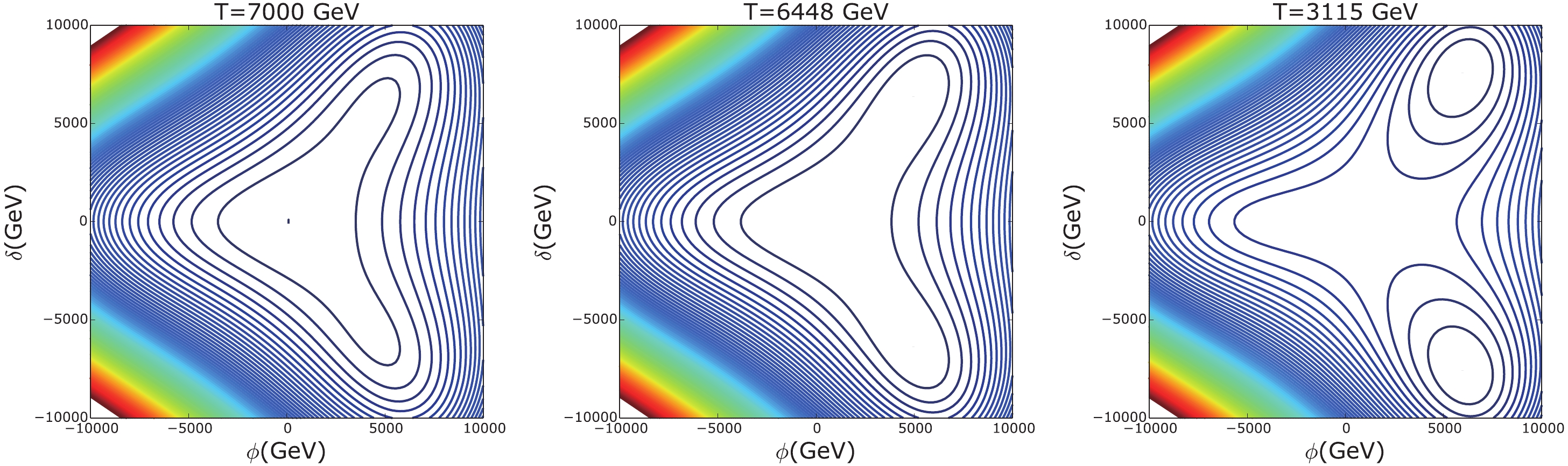

Figure 1

Figure 1.  (color online) Contours of the effective potential of model (b) at three typical temperatures, with blue lines for lower values and red for higher values. The left figure is at a temperature higher than $T_C \approx 6448$ GeV, the middle one is at $T_C$, and the right figure is at $T_n \approx 3115$ GeV. The benchmark parameters are: $v_{\phi}=4637$ GeV, $v_{\delta} = 1902$ GeV, $\theta = 0.128$, $m_{s_1} = 2400$ GeV, $m_{s_2} = 1236$ GeV, and $\Lambda = -2143$ GeV.

DownLoad: Full-Size Img PowerPoint

Figure 2

Figure 2.  (color online) Tracks of the minimum $(\phi \neq 0,$ $\delta \neq 0)$ in the $(\phi, \delta)$ plane, with the colors indicating the value of temperature, which can be read from the colormap on the left.

DownLoad: Full-Size Img PowerPoint

To calculate the GWs from this model, we need the input $\kappa_v$, which we calculate following Ref. [59]. For the benchmark given in Fig. 1, we find $\alpha = 0.09$, $\beta/H_n \approx 6$, and $\kappa_v$ depending on one free parameter $v_w$. For different values of $v_w$, the motion of the plasma surrounding the bubble takes different forms, and the value of $\kappa_v$ is shown in the left panel of Fig. 3, where representative points are marked as A, B, C, and D, shown as green points in the figure. The velocity profile of the plasma is depicted in the right panel of Fig. 3 as a function of $r/t$, where r is the radial distance from the bubble center and t starts at $T_n$. For case A, $v_w$ is smaller than the speed of sound in the plasma ($\equiv c_s = 1/\sqrt{3}$, the vertical dashed line in left panel), and the bubble proceeds as deflagrations, with a velocity profile shown by the dotted lines in the right panel. For case B, $v_w$ is larger than $c_s$, a rarefaction wave develops behind the bubble wall, yet the fluid has non-zero velocity ahead of the wall, indicated as the solid lines in the right panel. This falls within the hybrid region of the left panel, denoting supersonic deflagration [71]. For case C, $v_w$ is increased to the Jouguet detonation [72] (the magenta dotted line in the left panel) and the velocity of the fluid ahead of the wall becomes zero, indicated as the dashed line in the right panel. For case D, the bubble wall velocity becomes larger and the expansion takes the form of detonation with the profile depicted by the dot-dashed line in the right panel. For these four choices of $v_w$, we find $\bar{U}_f \approx$ 0.12, 0.09, 0.09, and $0.07$, respectively. From Eq. (28), it follows that $H_n \tau_{\rm{sh}} \approx$ 1.56, 3.24, 4.03, and 5.85, respectively. Because all these values are larger than 1, there is no need to consider the suppression caused by the early onset of shocks and turbulence. For smaller values of $v_w$, $H_n \tau_{\rm{sh}}$ decreases. More precisely, for this choice of $\alpha$, we have $H_n \tau_{\rm{sh}}<1$ when $v_w < 0.25$, and one needs to consider this suppression. The other reduction effect, found in Ref. [62], is small for these benchmarks, because $\alpha$ is small (see Fig. 6 of Ref. [62] or see Fig. 2 of Ref. [73] for this reduction factor on the $(v_w, \alpha)$ p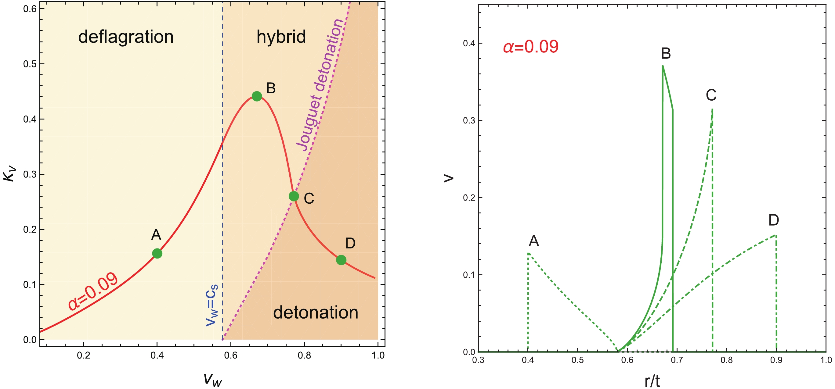lane).

Figure 3

Figure 3.  (color online) Left panel: The red line shows the fraction of latent heat transferred to the bulk motion of the plasma $\kappa_v$ when the bubble wall velocity is varied for $\alpha=0.09$, which is derived the benchmark in Fig. 1. Also plotted here are the deflagration, hybrid(supersonic deflagration), and detonation regions characterizing the dynamics of the phase transition, separated by the blue dashed line (when $v_w$ is equal to the speed of sound of the relativistic plasma $c_s = 1/\sqrt{3}$) and the magenta dotted line (Jouguet detonation). Four representative cases: A, B, C and D, marked with green points, are chosen to calculate the GW spectra. Right panel: The velocity profile as a function of $r/t$ for the four representative cases of the left panel plot.

DownLoad: Full-Size Img PowerPoint

The resulting GW energy spectra for these four points from sound waves (blue dashed) and turbulence (brown dotted) are depicted in Fig. 4, where their sum corresponds to the red solid line. The color-shaded regions at the top are the experimental sensitivity regions for the LISA configurations C1 (red), Tianqin (yellow), Taiji (gray), DECIGO (brown), BBO (green), and Ultimate-DECIGO (purple). It is observed that, for all four cases, the spectrum at around the peak frequency is dominated by sound waves, whereas turbulence becomes more important for large and small frequencies. The total GW spectra all fall within the experimental sensitive regions of the LISA configuration as well as other experiments. To assess the discovery prospect of the GWs, we quantify the detectability of the GWs using the signal-to-noise ratio adopted in Ref. [15]:

Figure 4

Figure 4.  (color online) GW energy spectrum as function of its frequency for the benchmark in Fig. 1, and four representative bubble wall velocities (the four green points A, B, C, and D in Fig. 3). The individual contributions from sound waves and turbulence are plotted using blue dashed and brown dotted lines, respectively, with their sum given as the red solid line. Also plotted are the experimental sensitive regions at the top, corresponding to color-shaded regions, from the LISA detector with C1 configuration, Tianqin (yellow), Taiji (gray), DECIGO (brown), BBO (green), and Ultimate-DECIGO(purple).

DownLoad: Full-Size Img PowerPoint

where $h^2 \Omega_{{\rm{exp}}}$ is the experimental sensitivity depicted in Fig. 4 and ${\cal{T}}$ is the mission duration of the experiment in years. For all cases, we set ${\cal{T}} = 5$. With this formula, we calculate SNR as a function of $v_w$ for each experiment and present the results in Fig. 5. Note that $v_w$ can take the full range of values between 0 and 1. One needs to check the suppression factor ${\cal{S}}$. As discussed earlier, this affects mainly the region $v_w \leqslant 0.25$ for this choice of $\alpha$ and leads to a slight reduction in the gravitational wave signal and thus the SNR. We incorporate this suppression in our calculations. For the other reduction as recently observed in Ref. [62], its effect is minor because $\alpha$ is quite small and is neglected in this study. We also demonstrate two representative SNR thresholds ${\rm{SNR}}_{{\rm{thr}}} = 10, 50$ as suggested by Ref. [15] with horizontal black lines for comparison. From this figure, we can see that all SNR curves have a peak at $v_w \approx 0.67$. This peak corresponds to the maximum of $\kappa_v \approx 0.44$ in the left panel of Fig. 3, represented by case B in previous discussion, which has a supersonic deflagration profile of the plasma surrounding the bubble. It is clear from this figure that, for a wide range of $v_w$, the SNR for the LISA configuration C1, Tianqin, BBO, and UDECIGO are above the two thresholds ${\rm{SNR}}_{{\rm{thr}}} = 10, 50$. For DECIGO, there is also a range $0.5 \lesssim v_w < 0.8$ above threshold 50, and this range becomes much wider for threshold 10. For Taiji, there is a window at $v_w \approx 0.7$ where the SNR is above 10. We note that these SNRs are obtained assuming a mission duration of $5$ years. Also note that the used sensitivity curves depend on the specific detector configurations proposed, such as the arm length and noice level achieved. All these are subject to change if the eventual configurations are changed.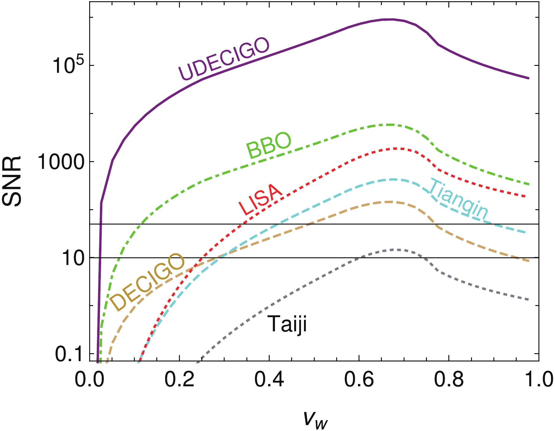

Figure 5

Figure 5.  (color online) SNR as function of bubble wall velocity $v_w$ for the benchmark point in model (b) using the different experimental sensitivity inputs. Two black horizontal lines denote SNR threshold values of 10 and 50, respectively.

DownLoad: Full-Size Img PowerPoint

4. Discussion

• 1. Introduction
• 2. Abelian gauge group extensions to SM
•      2.1 Model (a)
•      2.2 Model (b)
• 3. Gravitational wave signals
• 4. Discussion

The discovery of GW at LIGO heralds a new era in high-energy physics and gravity. In this paper, we proposed the stochastic GW as an indirect way of probing the spontaneous breaking new gauge symmetry beyond the SM. Working with models with the gauged ${{\bf{B}}-{\bf{L}}}$ extension of the SM, we studied the strength of PT relating to the spontaneous breaking of the ${{\bf{B}}-{\bf{L}}}$ as well as the stochastic GW signals generated during the same PT in the space-based interferometer. We found that the power spectrum of GW generated is reachable by LISA, Tianqin, Taiji, BBO, DECIGO, and Ultimate-DECIGO for the case where the spontaneous breaking of ${{\bf{B}}-{\bf{L}}}$ is triggered by at least two electroweak scalar singlets. It should be mentioned that there is no way to identify its intrinsic physics if any stochastic GW signal is observed. However, it provides a guidance for new physics hunters because the stochastic GW signal with peak frequency at near $0.01\; {\rm{Hz}}$ hints at new scalar interactions or new symmetry at the TeV scale. This study makes sense of this point of view. Although we focused only on the $U(1)$ case in this study, our results can be easily extended to the non-Abelian case because it contains all ingredients of the GW calculation.

References