Radiative decays of f₁(1285) as the ${ { K}^*\bar { K}}$ molecular state

1. Introduction

• 1. Introduction
• 2. Formalism
•      2.1 Effective interactions and coupling constants
•      2.2 Decay amplitudes
•      2.3 The $\rho^0$ width contributions
• 3. Numerical results and discussion
• 4. Summary

The radiative decay mode of the $f_1(1285)$ resonance is interesting because it is the basic element in the description of the $f_1(1285)$ photoproduction data [1, 2]. It is also advocated as one of the observables most suitable for learning about the nature of the $f_1(1285)$ state [3-7]. Using the chiral unitary approach, $f_1(1285)$ appears as a pole in the complex plane of the scattering amplitude of the $K^* \bar K+c.c.$ interaction in the isospin $I = 0$ and $J^{PC} = 1^{++}$ channel [8-10]. In other words, the axial-vector meson $f_1(1285)$ can be taken as a $K^*\bar{K}$ molecular state. For brevity, we use $K^* \bar K$ to represent the positive C-parity combination of $K^* \bar K$ and $\bar{K}^* K$ in what follows.

The experimental decay width of $f_1(1285)$ is $22.7 \pm 1.1$ MeV [7], quite small compared with its mass. This is naturally explained in Ref. [8] using the molecular picture, implying that $f_1(1285)$ is a dynamically generated state. The $K^* \bar{K}$ channel is the only allowed and considered pseudoscalar-vector channel in the chiral unitary approach, and the pole of $f_1(1285)$ is below the $K^* \bar{K}$ threshold; therefore, the total width of the $f_1(1285)$ resonance was not obtained in Ref. [8]. If the convolution of the $K^*$ width was taken into account, the partial decay width of the $K^*\bar{K}$ channel would be approximately $0.3$ MeV (see more details in Ref. [8]). In fact, the dominant decay modes contributing to the width are peculiar. For example, the $\eta \pi \pi$ channel accounts for 52% of the width, and the branching ratio of $\pi a_0(980)$ channel is 38%. The decay of $f_1(1285) \to \pi a_0(980)$ has been well investigated in Ref. [11] within the $K^*\bar{K}$ molecular state picture for $f_1(1285)$. These theoretical calculations in Ref. [11] have been confirmed in a recent BESIII experiment [12].

There is another important decay channel, i.e., the $K \bar K \pi$ channel, the branching ratio of which is $(9.1\pm 0.4)$% [7]. This decay mode was investigated in Ref. [13] with the same picture as in Ref. [11], and the theoretical predictions agree with existing experimental data. One could posit that the decay of $f_1(1285)\to \bar{K}K^* \to K\bar{K}\pi$ should be much enhanced, owing to the strong coupling of $f_1(1285)$ to the $\bar{K}K^*$ channel. Actually, the mass of $f_1(1285)$ is below the mass threshold of $\bar{K}K^*$; hence, it is easy to see that the above mechanism is much suppressed owing to the highly off-shell effect of the $K^*$ propagator, which was already found and discussed in Ref. [13] (see more details in that reference). Yet, all of the above tests have been performed for hadronic decay modes and not for radiative decays. In this work, we study the radiative decays of the $f_1(1285)$ resonance, assuming that it is a $K^*\bar{K}$ state.

On the experimental side, the particle data group (PDG) averaged values for the radiative decays of $f_1(1285)$ are [7]^①

which leads to the partial decay width $\Gamma_{f_1 \to \gamma \rho^0} = 1.2 \pm 0.3$ MeV and a ratio $R_1 = {\rm{Br}}(f_1 \to \gamma \rho^0)/{\rm{Br}}(f_1 \to \gamma \phi) = 71 \pm 30$. There is currently no experimental data on the $f_1(1285) \to \gamma \omega$ decay. On the other hand, the recent value of $\Gamma_{f_1 \to \gamma \rho^0}$ obtained by the CLAS collaboration at Jafferson Lab, utilizing the analysis of the $\gamma p \to p f_1(1285)$ reaction, is much smaller, at $0.45 \pm 0.18$ MeV [1]. These values were obtained with ${\rm{Br}}(f_1 \to \eta \pi \pi) = 0.52 \pm 0.02$ [7]; the measured branching ratio was ${\rm{Br}}(f_1 \to \gamma \rho^0)/$${\rm{Br}}(f_1 \to \eta \pi \pi) = 0.047 \pm 0.018$ and the width was $\Gamma_{f_1} =$$18.4 \pm 1.4$ MeV in Ref. [1]. The measured mass of the $f_1(1285)$ state was $M_{f_1} = 1281.0 \pm 0.8$ MeV, compatible with the known properties [7] of the $f_1(1285)$ resonance. On the theoretical side, the authors in Ref. [2] report $\Gamma_{f_1 \to \gamma \rho^0} = 0.311$ MeV and $\Gamma_{f_1 \to \gamma \omega} = 0.0343$ MeV under the assumption that $f_1(1285)$ has a quark-antiquark nature. This $\Gamma_{f_1 \to \gamma \rho^0}$ value is compatible with that obtained by the CLAS collaboration, within the error range, but is much smaller than the above PDG averaged value. Within the picture of $f_1(1285)$ being a quark-antiquark state, another theoretical prediction for the $f_1(1285)$ radiative decay was reported in Ref. [14] using a covariant oscillator quark model. It predicted $\Gamma_{f_1(1285) \to \gamma \rho^0}$ in the range of 0.509~0.565 MeV, $\Gamma_{f_1(1285) \to \gamma\omega}$ in the range of 0.048~0.057 MeV, and $\Gamma_{f_1(1285) \to \gamma\phi}$ in the range of 0.0056~0.02 MeV; these predictions depend on a particular mixing angle between the $(u\bar{u} + d\bar{d})/\sqrt{2}$ and $s\bar{s}$ components. Note that $f_1(1285)$ and $f_1(1420)$ are the members of the pseudovector nonet in the $q\bar{q}$ quark model [2, 14], where $f_1(1285)$ is a mostly $u\bar{u} + d \bar{d}$ state and $f_1(1420)$ is an $s\bar{s}$ state. However, the study in Ref. [15] shows that $f_1(1420)$ is not a genuine resonance and it shows up as a peak because of the $K^*\bar{K}$ and $\pi a_0(980)$ decay modes of $f_1(1285)$ around $1420$ MeV. In fact, as discussed by the PDG [7], although these two states are well known, their nature remains to be established. Thus, further investigations about them are needed [16].

Here, we extend the work in Refs. [11, 13] for the hadronic decays of $f_1(1285)$ to the case of radiative decays. In the molecular state scenario, $f_1(1285)$ decays into $\gamma V$ ($V = \rho^0$, $\omega$, and $\phi$) via kaon loop diagrams, and we can evaluate simultaneously these processes. It is shown that the theoretical results are in a good agreement with experimental data, hence supporting the strong coupling of the $f_1(1285)$ state to the $\bar{K} K^*$ channel.

The present paper is organized as follows. In Sec. 2, we discuss the formalism and the main ingredients of the model. In Sec. 3 we present our numerical results and conclusions. A short summary is given in the last section.

2. Formalism

• 1. Introduction
• 2. Formalism
•      2.1 Effective interactions and coupling constants
•      2.2 Decay amplitudes
•      2.3 The $\rho^0$ width contributions
• 3. Numerical results and discussion
• 4. Summary

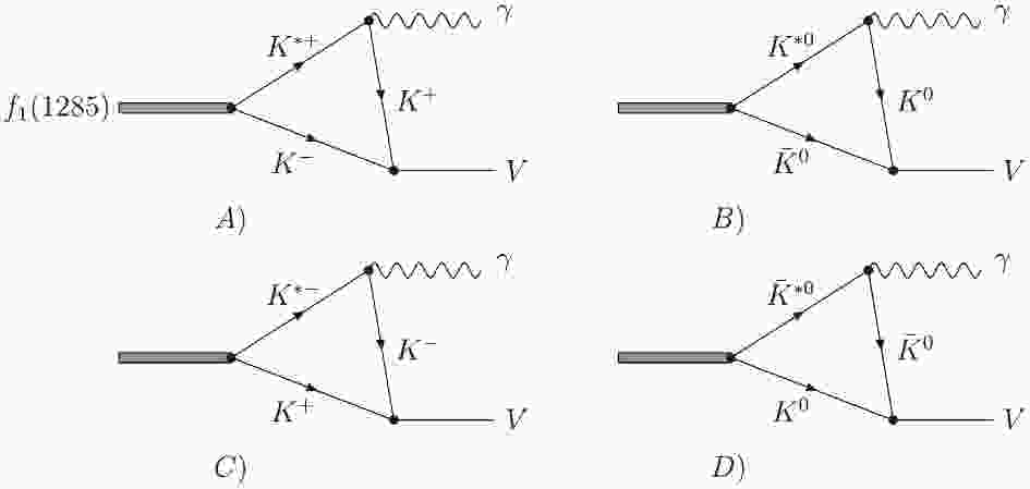
We study the $f_1(1285) \to \gamma V$ decays under the assumption that $f_1(1285)$ is dynamically generated from the $K^* \bar{K} + c.c.$ interaction; thus, this decay can proceed via $f_1(1285) \to K^* \bar{K} \to \gamma V$ through triangle loop diagrams, which are shown in Fig. 1. In this mechanism, $f_1(1285)$ first decays into $K^* \bar{K}$, then $K^*$ decays into $K \gamma$, and $K\bar K$ interacts to produce the vector meson V in the final state. We use p, k, and q for the momentum of $f_1(1285)$, $\gamma$ and $K^-$ and $\bar{K}^0$ in Figs. 1 (a, b) , respectively. Then, one can easily obtain that the momentum of the final vector meson is $p-k$, and the momenta of $K^*$ and K are $p-q$ and $p-q-k$, respectively. On the other hand, the decay of $f_1(1285) \to \gamma V$ can also go with $K^*$ exchange, where one needs a $K^*K^*\gamma$ vertex; then, $K^*\bar{K}$ interacts to produce the vector meson V. However, it is easy to see that, compared with the mechanism shown in Fig. 1, this mechanism is strongly suppressed owing to the highly off-shell effect of the exchanged $K^*$ propagator when the $K^*\bar{K}$ invariant mass is the mass of the vector meson V. In fact, as shown in Ref. [17], for the case of $a_1/b_1 \to \gamma \pi$ decays, the contribution of the $K^*$ exchange is rather small, on the order of 0.5%, compared with the one from the K exchange. Therefore, it is expected that the contributions from the $K^*$ exchange will be also small for the $f_1 \to \gamma V$ decays, as studied here, and those contributions can be safely neglected.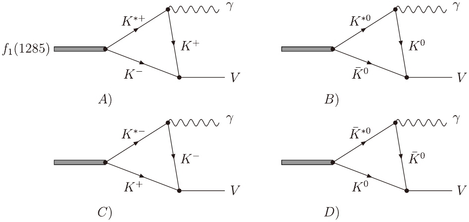

Figure 1

Figure 1.  Triangle loop diagrams representing the process $f_1(1285) \to \gamma V$ , with V being the $\rho^0$, $\omega$, or $\phi$ meson.

DownLoad: Full-Size Img PowerPoint

2.1 Effective interactions and coupling constants

• 1. Introduction
• 2. Formalism
•      2.1 Effective interactions and coupling constants
•      2.2 Decay amplitudes
•      2.3 The $\rho^0$ width contributions
• 3. Numerical results and discussion
• 4. Summary

To evaluate the radiative decay of $f_1(1285) \to \gamma V$, we need the decay amplitudes of these diagrams, shown in Fig. 1. As mentioned above, the $f_1(1285)$ resonance is dynamically generated from the interaction of $K^* \bar{K}$. For the charge conjugate transformation, we take the phase conventions $\mathcal{C}K^* = - \bar{K}^*$ and $\mathcal{C}K = \bar{K}$, which are consistent with the standard chiral Lagrangians, and write

Then we can write the $f_1(1285)\bar{K}K^*$ vertex as

where $\epsilon^{\mu}(f_1)$ and $\epsilon_{\mu}(K^*)$ stand for the polarization vector of $f_1(1285)$ and $K^*$ ($\bar{K}^*$), respectively. We will take the value of the coupling constant of $g_{f_1 \bar{K} K^*} (\equiv g_{f_1} = 7555\; \rm{MeV})$ as obtained in the chiral unitary approach [8]. The factors $C_1$ account for the weight of each $\bar{K}K^*$ ($K\bar{K}^*$) component of $f_1(1285)$, corresponding to the $f_1 \bar{K}K^*$ vertex for each diagram shown in Fig. 1, and can be easily obtained from Eq. (3) as,

For the $\bar K K V$ vertices, we take the effective Lagrangian describing the pseudoscalar-pseudoscalar-vector (${\rm PPV}$) interaction as [18-21],

where $g = M/{2f} = 4.2$ with $M \approx (m_{\rho} + m_{\omega})/2$ and $f = 93$ MeV. The symbol $<>$ denotes the trace, while the pseudoscalar- and vector-nonets are collected in the P and V matrices, respectively. We can write them as

and

with $\xi_1 = \frac{1}{\sqrt{2}} \pi^0 + \frac{1}{\sqrt{3}} \eta + \frac{1}{\sqrt{6}} \eta'$, $\xi_2 = - \frac{1}{\sqrt{2}} \pi^0 + \frac{1}{\sqrt{3}} \eta + \frac{1}{\sqrt{6}} \eta'$, and $\xi_3 = - \frac{1}{\sqrt{3}} \eta + \frac{2}{\sqrt{6}} \eta'$.

Thus, the $\bar K K V$ vertex can be written as

where $\varepsilon_{\mu}(p-k,\lambda_V)$ is the polarization vector of the vector meson. From Eq. (6) and from the explicit expressions for the V and P matrices as shown in Eqns. (7) and (8), the factors $C_2$ for each diagram shown in Fig. 1 can be obtained,

In terms of Eqns. (5) and (10), it is easy to see that Figs. 1 (a, c) give the same contribution and Figs. 1 (b, d) also give the same contribution. We hence only consider Figs. 1 (a, b) in the following calculation.

In addition, according to the Lagrangian in Eq. (6), the $\phi \to K\bar K$ decay width is given by

and we can obtain the coupling $g \simeq 4.5$ with the averaged experimental value of $\Gamma_{\phi \to K \bar K} = 1.77 \pm 0.02$ MeV, $m_\phi = 1019.46$ MeV, and $m_K = (m_{K^+} + m_{\bar{K}^0})/2 = 495.6$ MeV as quoted by the PDG [7]. Hence, in this work, we will take $g = 4.2$ as in Eq. (6).

For the electromagnetic vertex $K^* K \gamma$, the effective interaction Lagrangian takes the form as in Refs. [22-25]

where $K^*_\nu$, $A_\beta$ and K denote the $K^*$ vector meson, photon, and the K pseudoscalar meson, respectively. The partial decay width of $K^* \to K \gamma$ is given by

The values of the coupling constants $g_{K^*K\gamma}$ can be determined from the experimental data [7], $\Gamma_{K^{*+} \to K^+ \gamma} = 50.3 \pm 4.6$ keV and $\Gamma_{K^{*0} \to K^0 \gamma} = 116.4 \pm 10.2$ keV, which lead to

where the small errors are determined with the uncertainties of $\Gamma_{K^* \to K\gamma}$ as above. In addition, we fix the relative phase between the above two couplings, taking into account the quark model expectation [26].

2.2 Decay amplitudes

• 1. Introduction
• 2. Formalism
•      2.1 Effective interactions and coupling constants
•      2.2 Decay amplitudes
•      2.3 The $\rho^0$ width contributions
• 3. Numerical results and discussion
• 4. Summary

The partial decay width of the $f_1(1285) \to \gamma \rho^0$ decay is given by

where $M_A$ and $M_B$ are the decay amplitudes in Figs. 1 (a, b), respectively, and the energy of the photon is $E_\gamma = |\vec{k}\; | = ({M^2_{f_1} - m^2_{\rho^0}})/{2M_{f_1}}$. In the cases of $\omega$ and $\phi$ production, these can be obtained in a straightforward manner.

The above amplitudes, $M_A$ and $M_B$, can be easily obtained with effective interactions. Here, we give explicitly the amplitude $M_A$ for the $\rho^0$ production,

where $\omega^*(q) = \sqrt{|\vec{q}\; |^2 + m^2_{K^{*+}}}$ is the $K^{*+}$ energy, and we have taken the positive energy part of the $K^*$ propagator into account, which is a good approximation, given the large mass of $K^*$ (see more details in Ref. [11]). In Eq. (15), the factors $D_1$ and $D_2$ read^②

with $\lambda_{f_1}$, $\lambda_\gamma$, and $\lambda_{\rho}$ the spin polarizations of $f_1(1285)$, photon, and $\rho^0$ meson, respectively. The amplitude $M_B$ corresponding to Fig. 1 (b) can be easily obtained through the substitutions $m_{K^{*+}} \to m_{K^{*0}}$, $m_{K^+} \to m_{K^0}$, and $m_{K^-} \to m_{\bar{K}^0}$ into $M_A$. The decay amplitudes of $f_1(1285)\to\gamma\phi$ and $f_1(1285)\to\gamma\omega$ share the similar formalism as in Eq. (15).

To calculate $M_A$ in Eq. (15), we first integrate over $q^0$ using Cauchy's theorem. For doing this, we take the rest frame of $f_1(1285)$, in which one can write

with $\theta$ and $\phi$ as the polar and azimuthal angles of $\vec{q}$ along the $\vec{k}$ direction. The energy of the final vector meson is $E_V = (M^2_{f_1} + m^2_V)/2M_{f_1}$. Then, we have

for $\lambda_{f_1} = 0$, $\lambda_\gamma = \pm 1$, and $\lambda_{\rho} = \mp1$, and

for $\lambda_{f_1} = \pm 1$, $\lambda_\gamma = \pm 1$, and $\lambda_{\rho} = 0$. Notice that we have dropped those terms containing ${\rm sin}\phi$ or ${\rm cos}\phi$, because after the integration over the azimuthal angle $\phi$, they do not yield contributions.

After integrating over $q^0$ in Eq. (15), we have

where

with $\omega^\prime = \sqrt{|\vec{q}\; |^2 + E^2_\gamma +2E_\gamma |\vec{q}\; |{\rm cos}\theta +m^2_{K^+}}$ and $\omega = \sqrt{|\vec{q}\; |^2 + m^2_{K^-}}$ the energies of $K^-$ and $K^+$ in the diagram of Fig. 1 (a). $F^B_1$ and $F^B_2$ will be obtained just by applying the substitution to $F^A_1$ and $F^A_2$ with $m_{K^{*+}} \to m_{K^{*0}}$, $m_{K^-} \to m_{\bar{K}^0}$, and $m_{K^+} \to m_{K^0}$.

Finally, the partial decay width takes the form

with

For $\rho^0$ production, the relative minus sign between $C_A$ and $C_B$ combined with the minus sign between the couplings $g_{K^{*+} K^+ \gamma}$ and $g_{K^{*0} K^0 \gamma}$ is positive, and hence the interference of the two diagrams $(a)$ and $(b)$ shown in Fig. 1 is constructive. However, it is destructive for $\omega$ and $\phi$ production, which make $\Gamma_{f_1(1285) \to \gamma \rho^0}$ much larger compared with the other two partial decay widths.

In Eq. (24), we have introduced a momentum cutoff $\Lambda$ for preventing the ultraviolet divergence and for compensating the off-shell effects that appear in the triangle loop integral. It can also be done by introducing form factors to the intermediate particles, as shown in Refs. [27-32].

Again, we want to stress that, in this work, those contributions of the $K^*$ exchange via diagrams containing anomalous vector-vector-pseudoscalar (VVP) vertices are not taken into account.^③ Such contributions were extensively studied in Refs. [17, 33-35] for the low-lying scalar, axial vector, and tensor meson radiative decays. As discussed in Refs. [33, 34], these contributions are very sensible to the exact value of the VVP coupling. Furthermore, including such diagrams, the decay amplitudes would become more complex, owing to additional model parameters, which cannot be exactly determined. Hence, we leave these contributions to further studies when more precise experimental measurements become available.

2.3 The $\rho^0$ width contributions

• 1. Introduction
• 2. Formalism
•      2.1 Effective interactions and coupling constants
•      2.2 Decay amplitudes
•      2.3 The $\rho^0$ width contributions
• 3. Numerical results and discussion
• 4. Summary

In this section, we explain how the large $\rho^0$ width contributions are implemented. We study $f_1(1285) \to \gamma \rho^0$ with the $\rho^0 \to \pi^+\pi^-$ decay. For this purpose we replace $\Gamma_{f_1 \to \gamma \rho^0}$ in Eq. (24) by $\overline{\Gamma}_{f_1 \to \gamma \rho^0}$:

where $\tilde{m}$ is the invariant mass of the $\pi^+\pi^-$ system. Then, ${\cal S}(\tilde m)$ has the form

where $\Gamma_{\rho}(\tilde{m})$ is energy-dependent, and it can be written as [36-42],

with $m_{\rho^0} = 775.26$ MeV, $\Gamma^0_{\rho^0} = 149.1$ MeV and $m_\pi = m_{\pi^+} = m_{\pi^-} = 139.57$ MeV.

3. Numerical results and discussion

• 1. Introduction
• 2. Formalism
•      2.1 Effective interactions and coupling constants
•      2.2 Decay amplitudes
•      2.3 The $\rho^0$ width contributions
• 3. Numerical results and discussion
• 4. Summary

The partial decay width of the $f_1(1285) \to \gamma V$ decay as a function of $\Lambda$ from 800 to 1500 MeV is illustrated in Fig. 2, where the black solid, dashed, and dotted curves stand for the theoretical results of the$\rho^0$, $\omega$, and $\phi$ production. It is worth mentioning that the results for $\omega$ and $\phi$ are multiplied by a factor of 100, while the red solid line stands for the results for the $\rho^0$ production but with the contributions of the $\rho^0$ mass as in Eq. (30). One can see that, from Fig. 2, the theoretical results have the same order of magnitude within the given range of the cutoff parameter $\Lambda$ values. In the considered range of cutoffs, $\Gamma_{f_1 \to \gamma \rho^0}$ varies from $0.4$ to $0.9$ MeV, which is consistent with the experimental result within the error range [1, 7]. In addition, the contribution of the $\rho^0$ width is also important and it will reduce the numerical results of $\Gamma_{f_1 \to \gamma \rho^0}$ by a factor of 18%.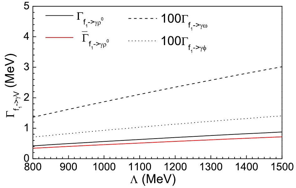

Figure 2

Figure 2.  (color online) Partial decay width of the $f_1(1285) \to \gamma V$ decay as a function of the cutoff parameter $\Lambda$. The black solid, dashed, and dotted curves denote the results for the $\rho^0$, $\omega$, and $\phi$ production, while the results for $\omega$ and $\phi$ are multiplied by a factor of 100. The red solid line denotes the results for the $\rho^0$ production but with the contributions of the $\rho^0$ mass as in Eq. (30).

DownLoad: Full-Size Img PowerPoint

In Table 1 we show explicitly the numerical results for the $f_1(1285) \to \gamma V$ decays with some particular cutoff parameters. We show also the theoretical calculations of Refs. [2, 14] and the experimental results [1, 7], for comparison.

Table 1

Table 1.  Partial decay width for $f_1(1285) \to \gamma V$. All units are in MeV.

$\Lambda$	$f_1 \to \gamma \rho^0$ $\Gamma$ ($\overline{\Gamma}$)	$f_1 \to \gamma \omega$ [$\times 10^{-2}$]	$f_1 \to \gamma \phi$ [$\times 10^{-2}$]	$R_1$	$R_2$
$800$	$0.42$ ($0.34$)	$1.36$	$0.71$	$59$	$31$
$1000$	$0.56$ ($0.46$)	$1.87$	$0.93$	$60$	$30$
$1500$	$0.88$ ($0.72$)	$3.01$	$1.41$	$62$	$29$
Ref. [2]	$0.311$	$3.43$	—	—	$9$
Ref. [14] (set I)④	$0.509$	$4.8$	$2.0$	$25$	$11$
Ref. [14] (set II)	$0.565$	$5.7$	$0.56$	$101$	$10$
Exp. [7]	$1.2 \pm 0.3$	—	$1.7 \pm 0.6$	$71 \pm 30$	—
Exp. [1]a	$0.45 \pm 0.18$	—	—	—	—
aThe measured width of $f_1(1285)$ is ~6 MeV smaller than the previous world average [7].

DownLoad: CSV

Show Table

In general, we cannot provide the value of the cutoff parameter; however, if we divide $\Gamma_{f_1(1285) \to \gamma \rho^0}$ by $\Gamma_{f_1(1285) \to \gamma \omega}$ or $\Gamma_{f_1(1285) \to \gamma \phi}$, the dependence of these ratios on the cutoff will be smoothed. Two ratios are defined as

These two ratios are correlated with each other. With $R_1$ measured experimentally, one can fix the cutoff in the model and predict the ratio $R_2$. We also show, in Table 1 , the explicit numerical results for $R_1$ and $R_2$ , for some particular cutoff parameters.

In Fig. 3, we show the numerical results for the above two ratios, where the solid line denotes the results for $R_1$, while the dashed line denotes the results for $R_2$. Indeed, one can see that the dependence of both ratios on the cutoff $\Lambda$ is rather weak. The ratio $R_1 \simeq 60$ is in agreement with the experimental result $71 \pm 30$ [7]. On the other hand, the result for $R_2$ is approximately $30$. We can conclude firmly that the partial decay width of $f_1(1285) \to \gamma \rho^0$ is much larger than the ones to $\gamma \omega$ and $\gamma \phi$ channels. This is owing to the destructive interference between Figs. 1 (a, b) for $\omega$ and $\phi$ production. Our present conclusion agrees wtih quark model calculations [2, 14]. However, from Table 1 one can see that the presently obtained ratios $R_1$ and $R_2$ are much different from the values obtained by the quark models, especially for $R_2$. In the quark model calculations, $R_2$ is always around $9$, which is owing to the isospin difference of $\rho^0$ and $\omega$ mesons. We hope that future experimental measurements will help to clarify this issue.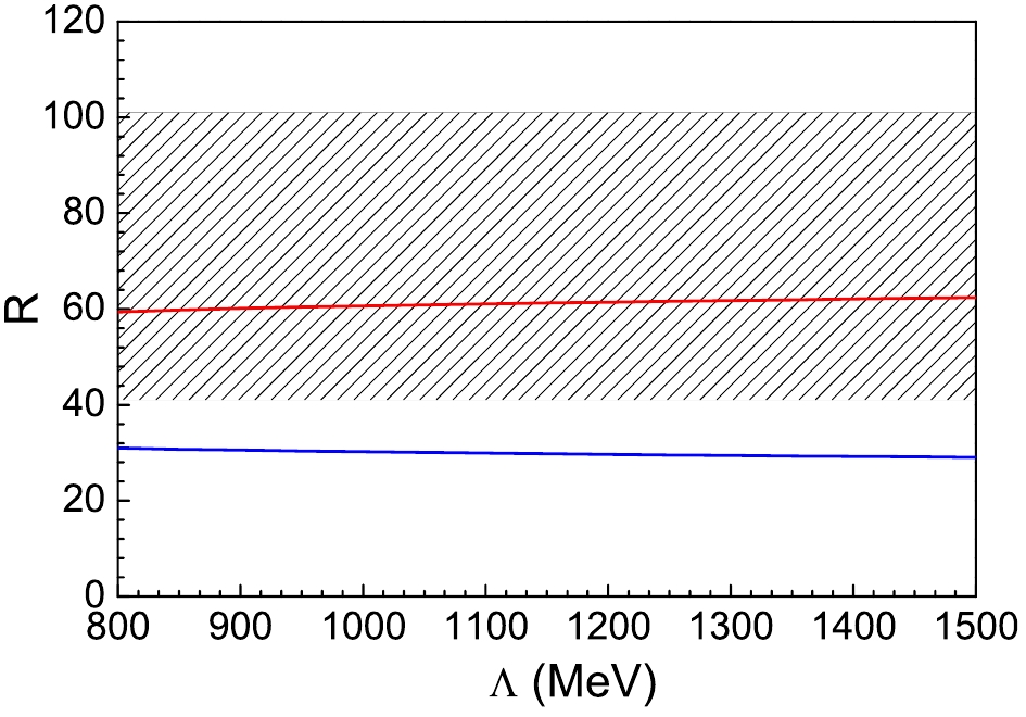

Figure 3

Figure 3.  (color online) The $\Lambda$ dependence of the ratios $R_1$ (solid line) and $R_2$ (dashed line) defined in Eq. (33). The error band corresponds to the experimental result for $R_1.$

DownLoad: Full-Size Img PowerPoint

It is worth mentioning that there is only one free parameter $\Lambda$ in the present work (all the other parameters were fixed in previous works). In addition, the dependence of $R_1$ and $R_2$ on the cutoff $\Lambda$ is rather weak; thus, these can be the model predictions, and they would be compared with future experimental measurements.

In addition, we want to note that, although we have assumed that $f_1(1285)$ is a dynamically generated state, the numerical results here are not tied to the assumed nature of $f_1(1285)$. The crucial point is that it couples strongly to the $\bar{K}K^*$ channel, whatever its origin.

4. Summary

• 1. Introduction
• 2. Formalism
•      2.1 Effective interactions and coupling constants
•      2.2 Decay amplitudes
•      2.3 The $\rho^0$ width contributions
• 3. Numerical results and discussion
• 4. Summary

We have evaluated the partial decay rates of the radiative decays $f_1(1285) \to \gamma V$ with the assumption that $f_1(1285)$ is a dynamically generated state from the strong $\bar K^* K$ interaction, and in this picture the $f_1(1285)$ state has a strong coupling to the $\bar{K}K^*$ channel. The theoretical results we obtained for the partial widths are sensitive to the free parameter $\Lambda$, but they are compatible with experimental data within the error range. Furthermore, the ratios $R_1 = \frac{\Gamma_{f_1 \to \gamma \rho^0}}{\Gamma_{f_1 \to \gamma \phi}}$ and $R_2 = \frac{\Gamma_{f_1 \to \gamma \rho^0}}{\Gamma_{f_1 \to \gamma \omega}}$, which are not sensitive to the only free parameter $\Lambda$, are predicted. It is found that the values of $R_1$ and $R_2$ obtained here are different from other theoretical predictions using quark models. The precise experimental observations of those radiative decays would then provide very valuable information about the relevance of the strong coupling of $f_1(1285)$ to the $\bar{K}K^*$ channel.

References