


 Abstract
 HTML
HTML Reference
 Related
 PDF
PDF


-
Since the discovery of the D-meson by the Mark I detector at the Stanford Linear Accelerator Center (SLAC) in 1976, experimentalists have performed substantial research about its properties. For example, the decay constant was measured by the Mark III detector at the SLAC [1], CLEO [2-4], and BES [5]; the corresponding branching fraction measurements were obtained from Mark III [6], Belle [7], CLEO-c [8], BABAR [9], and BES-III [10-12]; and the corresponding semileptonic form factors were determined by BES-III [13] and the HPQCD collaboration for the lattice results [14]. Recently, the BES-III collaboration updated the latest measurements for the D meson semileptonic decay into pseudoscalar
$ \pi $ and K-meson processes, i.e., the absolute branching fractions are$ {\cal{B}}(D^+ \to \bar K^0 e^+\nu_e) = 8.60(6)(15)\times10^{-2} $ ,$ {\cal{B}}(D^+ \to \pi^0 e^+\nu_e) = 3.63(8)(5)\times10^{-3} $ [15]. A brief review of the earlier work and current experimental status of D-meson decays can be found in Ref. [16].The D-meson is the lightest meson containing a single charm quark (antiquark) and has abundant decay channels. Among them, the heavy-to-light decay contains considerable information about the dynamics of weak and strong interactions [17], which may provide a platform to test the standard model more accurately and seek new physics (NP) beyond the SM. For example, the semileptonic decay
$ D\to P\ell\nu_\ell $ processes can be used to extract the Cabibbo-Kobayashi-Maskawa (CKM) matrix elements, which are an important part of the SM, as their associated decay branching fractions are proportional to the CKM matrix elements [18, 19]. Meanwhile, a single phase from the CKM quark mixing matrix dominates the CP violation phenomena [20], which is relevant to NP. Thus, the D-meson semileptonic decay is widely studied via various theoretic methods.The usual strategy for investigating D-meson semileptonic decay is to express the decay process as non-perturbative hadronic matrix elements with different
$ \gamma $ -structures, factorize them into Lorentz invariant transition form factors (TFFs) by employing covariant decomposition, and then study those TFFs using various theoretic methods, such as LCSRs [21-30], the transverse-momentum-dependent (TMD) factorization approach [31, 32], the lattice QCD [33-38], and the perturbative QCD [39-46]. As an alternative strategy, while the other processes remain unchanged, only the non-perturbative hadronic matrix elements are projected as the Lorentz invariant HFFs through the covariant helicity factor. The main difference between the latter and the usual TFFs arises from the use of different projection methods, which will bring some unique advantages to HFFs and may give better physical predictions. For more details, please see Refs. [47, 48]. For example, this method was used for dealing with the$ B \to \rho $ decays in our previous work [48], and the resultant differential decay width was found to be in good agreement with the BABAR experiment. Here, we will attempt to use HFFs within the framework of LCSR to study the$ D \to P(\pi,K) $ decays. Note that, in order to get more accurate LCSR results, our calculations for the$ D \to P(\pi,K) $ HFFs,$ {\cal{P}}_{0,t}^P(q^2) $ contain both LO and NLO contributions. For the LO contributions, two and three particles parts are contained up to twist-4 light-cone distribution amplitudes (LCDAs), while for the NLO contributions, one-loop gluon radiation correction is contained for the twist-(2,3) LCDAs.The remaining parts of the paper are organized as follows. In Sec. 2, we give a brief introduction for the definition of HFFs and provide the full LCSR expression for
$ {\cal{P}}^P_{0,t}(q^2) $ . In Sec. 3, we first discuss the hadron input parameters for HFFs and extrapolate those HFFs to the whole$ q^2 $ region by employing SSE. Then, we compute the differential decay width and branching fraction for$D\to $ $ P(\pi,K) $ decays from the HFFs. We compare our results with the available experimental results as well as other theoretical results. Finally, the conclusion is given in Sec. 4. -
The short distance hadronic matrix elements related to the pseudoscalar D-meson semileptonic deca
ys can be pr-ojected as the relevant HFFs via the off-shell W-boson po-larization vectors with 4-momentum $ q^\mu = (q^0,0,0,-|\vec q\,|) $ [47],$ {\cal{P}}_{\sigma}(q^2 )= \sqrt{\frac{q^2}{\lambda}} \, {\varepsilon_\sigma ^{*\mu}(q)} \, \langle P(k)|\bar q \, \gamma_\mu \, c |D(p)\rangle \,, $

(1) where the standard kinematic function
$\lambda = (t_- - $ $ q^2) (t_+ - q^2)$ with$ t_\pm = (m_D\pm m_P)^2 $ . The polarization vectors$ \varepsilon_\sigma ^{*\mu}(q) $ represent transverse ($ \sigma = \pm $ ), longitudinal ($ \sigma = 0 $ ), or time-like ($ \sigma = t $ ) components. More specifically,$ \varepsilon _ \pm ^\mu(q) = \mp \frac{1}{\sqrt 2 } (0,1, \mp i,0) , $

(2) $ \varepsilon _0^\mu (q) = \frac{1}{\sqrt {q^2 } } (|\vec q| ,0,0, - q^0 ) , $

(3) $ \varepsilon _t^\mu (q) = \frac{1}{\sqrt {q^2 } } q^\mu . $

(4) In order to derive the full analytical LCSRs expression for the HFFs, we take the following two-point correlation function as a starting point,
$ \begin{split} \Pi_\sigma(p,q) = & {\rm i} \sqrt{\frac{q^2}{\lambda}} {\varepsilon_\sigma^{*\mu}(q)} \\ & \times\int {\rm d}^4 x {\rm e}^{{\rm i}q\cdot x}\langle P(k)|T\{j_V^\mu(x),j_D^\dagger (0)\}|0\rangle, \end{split} $

(5) where the currents
$ j_V^\mu(x) = \bar {q}(x){\gamma _\mu } c(x) $ and$ j_D^\dagger (0) = \bar c(0)i \gamma_5 u(0) $ have the same quantum state as the pseudoscalar D-meson with$ J^{P} = 0^- $ . T stands for the product of the current operator.Following the basic procedure of LCSR, the correlation function can be treated by inserting complete intermediate states with the same quantum numbers as the current operator
$ \bar c i \gamma_5 u $ in the time-like$ q^2 $ -region. After isolating the pole term of the lowest pseudoscalar D-meson, one can obtain the following expression:$\begin{split} \Pi_\sigma ^H(p,q) =& \sqrt{\frac{q^2}{\lambda}} {\varepsilon_\sigma^{*\mu}(q)}\bigg[ \frac{ \langle P|\bar{q}\gamma _\mu c|D\rangle \langle D|\overline{c}{\rm i} \gamma_5 u|0\rangle} {m_D^2-(p+q)^2} \\[1ex] &+\sum\limits_{\rm{H}}\frac{\langle P|\bar{q}\gamma _\mu c|D^{\rm{H}}\rangle \langle D^{\rm{H}}|\bar{q}{\rm i}\gamma _5 u|0\rangle}{m_{D^{\rm{H}}}^2-(p+q)^2}\bigg], \end{split}$

(6) where
$\langle D|\bar{c}{\rm i}\gamma_5 u|0\rangle = m_D^2f_D/m_c$ . Employing dispersion integrations to replace the contributions of higher resonances and continuum states, the hadronic representation of the correlator$ \Pi^H_\sigma $ can be obtained$\begin{split} \Pi^H_\sigma(q^2,(p+q)^2) = &\frac{ m_D^2 f_D}{m_c [m_D^2-(p+q)^2]}{\cal{P}}_{\sigma}(q^2 )\\ & + \int _{s_0}^{\infty}\frac {\rho^{\rm{H}}_\sigma(s)}{s-(p+q)^2}{\rm d}s +{\rm{subtractions}}, \end{split}$

(7) where
$ s_0 $ is the effective threshold parameter, and the spectral densities$ \rho^{\rm{H}}_\sigma(s) $ can be approximated by employing the quark-hadron duality ansatz$ \rho ^{\rm{H}}_\sigma(s) = \rho_\sigma ^{\rm{QCD}}(s)\theta (s-s_0). $

(8) On the other hand, in the space-like
$ q^2 $ -region, i.e.,$ (p+q)^2-m_c^2\ll 0 $ and$ q^2\ll m_c^2-{\cal{O}}(1{{\rm{GeV}}^2}) $ , the correlation function can be pre-processed by contracting the c-quark operator to a free propagator,$ \begin{split} \langle0|c_\alpha^i(x)\bar c_\beta^j(0)|0\rangle = & -{\rm i}\int \frac{{\rm d}^4k}{(2\pi)^4}{\rm e}^{-{\rm i}k\cdot x}\bigg\{\delta^{ij}\frac{/\!\!\!k + m_c}{m_c^2-k^2} \\ & +g_s\int_0^1 {\rm d}v G^{\mu\nu\alpha}(vx)\left(\frac{\lambda}{2}\right)^{ij}\bigg[\frac{/\!\!\!k+m_c}{2(m_c^2 - k^2)^2}\sigma_{\mu\nu} \\ & + \frac1{m_c^2-k^2}vx_\mu\gamma_\nu\bigg]\bigg\}_{\alpha\beta}, \\[-15pt] \end{split} $

(9) where the nonlocal matrix elements are convoluted with the meson LCDAs with growing twist. The matrix elements can be expanded up to twist-4 LCDAs as follows [49]:
$ \langle P(p)|\bar q_1(x){\rm i}\gamma_5 u(0)|0\rangle = \frac{f_P m_P^2}{m_u + m_{q_1}} \int_0^1 {\rm d}u {\rm e}^{{\rm i}up\cdot x}\phi_{2;P}(u), $

(10) $ \begin{split} & \langle P(p)|\bar q_1(x)\gamma_\mu \gamma_5 u(0)|0\rangle = - {\rm i} p_\mu f_P \int_0^1 {\rm d}u {\rm e}^{{\rm i}up\cdot x}\bigg[\phi_{3;P}^p(u) \\ &\quad +x^2\psi_{4;P}(u)\bigg]+f_P(x_\mu-\frac{x^2p_\mu}{p \cdot x})\int_0^1 {\rm d}u {\rm e}^{{\rm i}up\cdot x}\phi_{4;P}(u), \end{split} $

(11) $\begin{split} &\langle P(p)|\bar q_1(x)\sigma_{\mu \nu} \gamma_5 u(0)|0\rangle = {\rm i}(p_\mu x_\nu - p_\nu x_\mu) \frac{f_P m_P^2}{6(m_u + m_{q_1})} \\ &\quad \times\int_0^1 {\rm d}u {\rm e}^{{\rm i}up\cdot x}\phi_{3;P}^\sigma(u), \end{split}$

(12) $ \begin{split} & \langle P(p)|\bar q_1(x)\sigma_{\mu\nu}\gamma_5 g_s G_{\alpha\beta}(vx)u(-x)|0\rangle = {\rm i} f_{3P} (p_\alpha p_\mu g_{\nu\beta}^\bot \\&\quad - p_\alpha p_\nu g_{\mu\beta}^\bot - (\alpha \leftrightarrow \beta))\Phi_{3;P}(v, p\cdot x), \end{split}$

(13) $ \begin{split} & \langle P(p) | \bar q_1(x)\gamma_\mu\gamma_5 gG_{\alpha\beta}(vx)u(-x)|0\rangle = p_\mu (p_\alpha x_\beta- p_\beta x_\alpha) \\ & \quad\times \frac{f_{P}}{p\cdot x} \Phi_{4;P}(v,p\cdot x) \\ & \quad + (p_\beta g_{\alpha\mu}^\perp -p_\alpha g_{\beta\mu}^\perp) f_{P}\Psi_{4;P}(v,p\cdot x), \end{split} $

(14) $ \begin{split} & \langle P(p) | \bar q_1(x)\gamma_\mu {\rm i} g\widetilde{G}_{\alpha\beta}(vx)u(-x)|0\rangle = p_\mu (p_\alpha x_\beta - p_\beta x_\alpha) \\ & \quad\times \frac{f_P}{p\cdot x} \widetilde\Phi_{4;P}(v,p\cdot x) \\ & \quad + (p_\beta g_{\alpha\mu}^\perp - p_\alpha g_{\beta\mu}^\perp) f_{P} \widetilde\Psi_{4;P}(v,p\cdot x), \end{split}$

(15) where P stands for
$ \pi,K $ -meson with$ q_1 = d,s $ quark, and we have set$ \begin{split} & g_{\mu\nu}^\bot = g_{\mu\nu} - \frac{p_\mu x_\nu + p_\nu x_\mu}{p\cdot x}, \\& K(v,p\cdot x) = \int_0^1 {\rm d}\alpha_1 {\rm d}\alpha_2 {\rm d}\alpha_3 \delta(1-\alpha_1-\alpha_2-\alpha_3) K(\alpha_i). \end{split}$

Here,
$ K(\alpha_i) $ stands for the twist-3 or twist-4 DA$ \Phi_{3;P}(\alpha_i) $ ,$ \Phi_{4;P}(\alpha_i) $ ,$ \Psi_{4;P}(\alpha_i) $ ,$ \widetilde\Psi_{4;P}(\alpha_i) $ and$ \widetilde\Psi_{4;P}(\alpha_i) $ . Furthermore, by replacing the non-local matrix elements and using dispersion integration to carry out the subtraction procedure of the continuum spectrum, the QCD representation can be obtained.After equating the two types of representations of the correlator and subtracting the contribution from higher resonances and continuum states, one can further carry out their Borel transformation, i.e., replacing the variable
$ (p + q)^2 $ with the Borel parameter$ M^2 $ and exponentiating the denominators, which removes the subtraction term in the dispersion relation and exponentially suppresses the contributions from unknown excited resonances. To obtain a higher calculation accuracy, we calculated the NLO gluon radiation correction corresponding to twist-(2,3) distribution amplitude for$ D \to P $ using the same method as that for the$ B\to \pi $ process [50]. The one-loop corrections may lead to amplitude divergence, which can be separated as UV divergence and infrared collinear divergence. The UV divergence will be canceled by the mass renormalization of heavy quark c and the infrared collinear divergence term can be absorbed by the evolution of the wave function of the meson [51]. Thus, the LCSR for the$ D \to P $ HFFs is finally obtained:$ \begin{split} {\cal{P}}^P_0(q^2) = & \frac{f_P m_c}{f_D m_D^2} \int_0^1 {\rm d} u {\rm e}^{(m_D^2 - s)/M^2} \bigg\{ m_c \bigg[ \frac{1}{2u} \Theta (c(u,s_0))\phi_{3;P}^p(u) - \frac{2m_c^2}{u^3M^4} \widetilde{\widetilde\Theta}(c(u,s_0))\psi_{4;P}(u) + \frac{1}{u M^2} \widetilde\Theta (c(u,s_0)) \phi_{4;P}(u) \\ & + \frac{2 m_c^2}{u^3 M^4} \widetilde{\widetilde\Theta}(c(u,s_0)) \Phi_{4I;P}(u) \bigg] +\frac{m_P ^2}{2(m_u + m_{q_1})}\bigg[\Theta (c(u,s_0)) \phi_{2;P}(u) + \bigg( \frac{1}{3u} \Theta (c(u,s_0)) + \frac{m_c^2 + q^2}{6u^2M^2} \widetilde\Theta (c(u,s_0))\bigg) \phi_{3;P}^\sigma(u) \bigg] \\ & - \frac{f_{3\pi}}{f_P }\frac{I_{3\pi}(u)}{u}- \frac{m_c}{2(m_c^2-q^2)}I_{4\pi}(u) \bigg\} + \frac{\alpha_s C_F}{8\pi m_D^2 f_D}F_1(q^2,M^2,s_0), \end{split}$

(16) $ \begin{split} {\cal{P}}^P_t (q^2) = & \frac{f_P m_c}{\sqrt \lambda f_D m_D^2 }\int_0^1 {\rm d} u {\rm e}^{(m_D^2 - s)/M^2} \bigg\{{\cal{Q}}_+ m_c \bigg[ \frac{1}{2u} \Theta (c(u,s_0))\phi_{3;P}^p(u) - \frac{2m_c^2}{u^3M^4} \widetilde{\widetilde\Theta}(c(u,s_0))\psi_{4I;P}(u) + \frac{1}{u M^2} \widetilde\Theta (c(u,s_0))\\& \times \phi_{4;P}(u)+ \frac{2 m_c^2}{u^3 M^4} \widetilde{\widetilde\Theta}(c(u,s_0)) \Phi_{4;P}(u) \bigg]+\frac{{\cal{Q}}_+m_P ^2}{2(m_u + m_{q_1})}\bigg[\Theta (c(u,s_0))\phi_{2;P}(u) + \bigg( \frac{1}{3u} \Theta (c(u,s_0)) + \frac{m_c^2 + q^2}{6u^2M^2} \\ & \times \widetilde\Theta (c(u,s_0))\bigg)\phi_{3;P}^\sigma(u) \bigg]+ q^2 \bigg[\frac{4 m_c}{u^2 M^2 } \widetilde\Theta (c(u,s_0))\phi_{4;P}(u) + \frac{2 m_P ^2}{u(m_u + m_{q_1})}\Theta (c(u,s_0))\phi _{2;P}(u)\bigg]\bigg\}+\frac{m_D^2-m_P^2}{\sqrt{\lambda}} \\ & \times\int_0^1 {\rm d}u {\rm e}^{(m_D^2 - s)/M^2}\frac{{\cal{Q}}_-}{m_D^2 - m_P^2}\bigg[-\frac{m_cf_{3P}}{u m_D^2 f_D}I_{3;P}(u) - \frac{m_c^2 f_P}{2m_D^2 f_D(m_c^2-q^2)}I_{4;P}(u)\bigg] +\frac{\alpha_s C_F}{4\pi}\; \frac{m_D^2-m_P^2}{2m_D^2 f_D\sqrt{\lambda}} \\ &\times \bigg[F_1(q^2,M^2,s_0) + \frac{q^2}{m_D^2-m_P^2}(\widetilde{F}_1(q^2,M^2,s_0) - F_1(q^2,M^2,s_0))\bigg], \end{split}$

(17) where P stands for
$ \pi,K $ -meson and$ {\cal{Q}}_\pm = q^2 \pm (m_D^2 - m_P^2) $ . The short-hand notations introduced for the integrals over three-particle DAs are$ \begin{split} & I_{3;P}(u) = \frac{{\rm d}}{{\rm d}u}\Bigg[\int\limits_0^u {\rm d}\alpha_1\!\!\!\int\limits_{\frac{(u-\alpha_1)}{(1-\alpha_1)}}^1 \!\! {\rm d}v \Phi_{3;P}(\alpha_i) \Bigg|_{\begin{array}{l} \alpha_2 = 1-\alpha_1-\alpha_3,\\ \alpha_3 = (u-\alpha_1)/v \end{array}}\Bigg]\,, \\ & I_{4;P}(u) = \frac{{\rm d}}{{\rm d}u}\Bigg\{\int\limits_0^u\! {\rm d}\alpha_1\!\!\! \int\limits_{\frac{(u-\alpha_1)}{(1-\alpha_1)}}^1 \!\! \frac{{\rm d}v}{v} \,\, \Bigg[2\Psi_{4;P}(\alpha_i)-\Phi_{4;P}(\alpha_i) \\ & \;\;\;\;\;\;\;\;\;\;\;\;\;\;\; +2\widetilde{\Psi}_{4;P}(\alpha_i)-\widetilde{\Phi}_{4;P}(\alpha_i)\Bigg] \Bigg|_{\begin{array}{l} \alpha_2 = 1-\alpha_1-\alpha_3,\\ \alpha_3 = (u-\alpha_1)/v \end{array} }\Bigg\}\,. \end{split} $

(18) The NLO terms in Eqs. (16) and (17) have the form of the dispersion relation:
$ \begin{split} &F_1(q^2,M^2,s_0) = \frac{1}{\pi}\int\limits_{m_c^2}^{s_0} {\rm d}s {\rm e}^{(m_D^2-s)/M^2}\,\rm{Im} F_1(q^2,s) \\ & = \frac{f_P}{\pi} \int\limits_{m_c^2}^{s_0}{\rm d}s {\rm e}^{(m_D^2-s)/M^2} \int_0^1 {\rm d}u\bigg \{ {\rm{Im}} T_1(q^2,s,u)\phi_{2;P}(u)\\ &\;\;\;\; + {\rm{Im}} T_1^p(q^2,s,u)\phi_{3;P}^p(u) + {\rm{Im}} T_1^\sigma(q^2,s,u)\phi_{3;P}^\sigma(u)\bigg \}, \end{split} $

(19) where the expressions of the imaginary parts of the amplitudes can refer to the
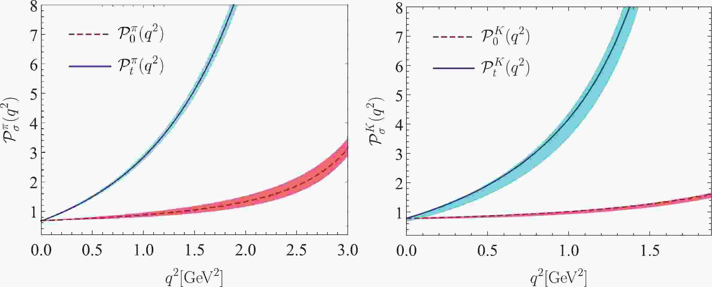
$ B\to \pi $ process [51]. The NLO amplitudes$ \widetilde{F}_1(q^2,s,u) $ have the same expression as$ T_1^{(p,\sigma)} (q^2,s,u) \to \widetilde T_1^{(p,\sigma)} (q^2,s,u) $ . At zero momentum transfer, the additional relation$ {\cal{P}}_t^P(0) = {\cal{P}}_0^P(0) $ holds, which can be confirmed not only from the abovementioned HFFs but also from Tables 3, 4 and Fig. 1.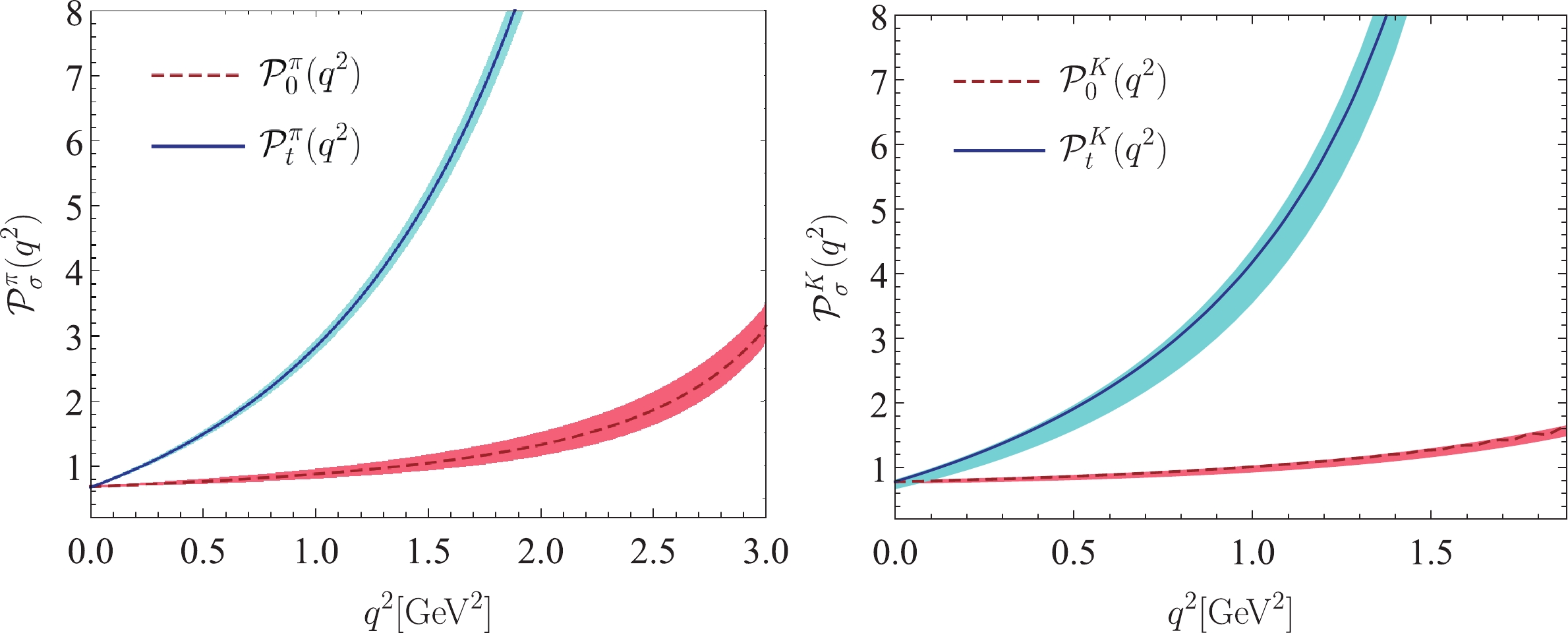
Figure 1. (color online) Extrapolated LCSR predictions for the
$ D \to \pi (K) $ HFFs$ {\cal{P}}_{0;t}^{P}(q^2) $ , in which the shaded bands are squared average of those from the mentioned error sources. -
In order to do the numerical calculations, we take the D, K, and
$ \pi $ -meson decay constants,$f_D = 0.2037\pm 0.0047\pm0.0006\; {\rm{GeV}}$ [52],$ f_K = 0.1555\; {\rm{GeV}} $ [53], and$ f_\pi = 0.1304\; {\rm{GeV}} $ [53], respectively. The c-quark pole mass$m_c = 1.28\pm0.03\; {\rm{GeV}}$ [54], the D, K, and$ \pi $ -meson masses$ {m_D} = 1.865\; {\rm{GeV}} $ ,$ {m_{K}} = 0.494\; {\rm{GeV}} $ , and$ {m_{\pi}} = 0.140\; {\rm{GeV}} $ [54], respectively. The factorization scale$ \mu $ is set as the typical momentum transfer of$ D \to K (\pi) $ , i.e.$\mu_{\rm{IR}} \simeq (m_{D}^2-m_c^2)^{1/2} \sim 1.3\; {\rm{GeV}}$ [55]. -
With regard to the hadron input about LCDAs, we will shortly discuss the twist-2,3,4 LCDAs. For the leading twist-2 LCDAs, we adopt a standard approach to do the calculation, i.e. the conformal expansion [49]:
$ \phi_{2;P}(u,\mu^2) = 6 u \bar u \left[ 1 + \sum\limits_{n = 1}^\infty a^P_{n}(\mu^2) C_{n}^{3/2}(\xi)\right], $

(20) where
$ \xi = 2u-1 $ ,$ \mu $ is the factorization scale, the superscript P represents the$ \pi $ and K-meson, and$ a^P_{n} $ is the (non-perturbative) Gegenbauer moment, which is usually up to the first two terms,$ a^P_{1,2} $ , accuracy due to the suppression of large n physical amplitudes of the Gegenbauer polynomials that oscillate rapidly.The two-particle twist-3 and twist-4 LCDAs
$ \phi_{3;P}^p(u) $ ,$ \phi_{3;P}^{\sigma}(u) $ ,$ \phi_{4;P}(u) $ ,$ \psi_{4;P}(u) $ , and$ \Phi_{4I;P}(u) $ are defined as follows [56]:$ \begin{split} \phi_{3;P}^p(u) =& 1+(30\eta_3^P - \frac{5}{2}\rho_{\pi}^2)C^{1/2}_2(\zeta)+(-3\eta_3^P \omega_3^P \\ & -\frac{27}{20}\rho_{\pi}^2-\frac{81}{10}\rho_{\pi}^2a_2^P)C^{1/2}_4(\zeta), \end{split} $

(21) $ \begin{split} \phi_{3;P}^{\sigma}(u) = & 6u(1-u)(5\eta_3^P - \frac{1}{2}\eta_3^P\omega_3^P - \frac{7}{20}\rho_{\pi}^2 -\frac{3}{5}\rho_{\pi}^2a_2^P) C^{3/2}_2(\zeta), \end{split}$

(22) $ \phi_{4;P}(u) = -m_P^2\int_0^u B(v){\rm d}v, $

(23) $ \psi_{4;P}(u) = \frac{1}{4}m_P^2 A(u) - \int_0^u \phi_{4;P}(v){\rm d}v, $

(24) $ \Phi_{4I;P}(u) = \int_0^u \phi_{4;P}(v){\rm d}v. $

(25) where
$ \begin{split} A(u) =& 6u\bar u \bigg[ \frac{16}{15} + \frac{24}{35} a_2^P + 20 \eta_3^P + \frac{20}{9}\eta_4^P + \bigg( -\frac{1}{15} \\ & + \frac{1}{16} - \frac{7}{27} \eta_3^P \omega_3^P - \frac{10}{27}\eta_4^P \bigg) C_2^{3/2}(\xi) + \bigg( -\frac{11}{210} \\ & \times a_2^P - \frac{4}{135} \eta_3^P \omega_3^P \bigg) C_4^{3/2}(\xi) \bigg]+ \bigg(-\frac{18}{5} a_2^P + 21 \\ & \times \eta_4 ^P\omega_4^P \bigg) \bigg[ 2u^3 (10-15 u + 6 u^2)\ln u + 2\bar u^3 (10 \\ & -15\bar u + 6 \bar u^2) \ln\bar u + u \bar u (2 + 13u\bar u)\bigg], \end{split}$

(26) $ \begin{split} B(u) = & 1+\left[1+\frac{18}{7}a_2^P + 60\eta_3^P + \frac{20}{3}\eta_4^P\right]C^{1/2}_2(\zeta) \\ & +\left[-\frac{9}{28}a_2^P - 6\eta_3^P\omega_3^P\right]C^{1/2}_4(\zeta). \end{split}$

(27) As for LO contributions, they do not mix under renormalization in the QCD theory; thus, the scaling up to
$ \mu_{\rm{IR}} $ is given by$ c_i(\mu_{\rm{IR}}) = {\cal{L}}^{\gamma_{c_i}/\beta_0} c_i(\mu_0) , $

(28) where
$ {\cal{L}} = \alpha_s(\mu_{\rm{IR}})/\alpha_s(\mu_0) $ ,$ \beta_0 = 11-2/3N_f $ , and the one-loop anomalous dimensions$ \gamma_{c_i} $ are given in Table 1 [56]. Given the initial scale$ \mu_0 $ values of the hadronic parameters [56], employing the renormalization function Eq. (28), one can obtain the corresponding values at the typical scale$ \mu = \mu_{\rm{IR}} $ ; our results are listed in Table 2.$ {\gamma_{a_n}}$ 

$ {C_F\left(1-\dfrac{2}{(n+1)(n+2)}-\sum\limits_{m=2}^{n+1}\dfrac{1}{m}\right)}$ 

$ {\gamma_{\eta_3}}$ 

$ {\dfrac{16}{3}C_F+C_A}$ 

$ {\gamma_{\eta_4}}$ 

$ {\dfrac{8}{3}C_F}$ 

$ {\gamma_{\omega_3}}$ 

$ {-\dfrac{25}{6}C_F+\dfrac{7}{3}C_A }$ 

$ {\gamma_{\omega_4}}$ 

$ {-\dfrac{8}{3}C_F+\dfrac{10}{3}C_A}$ 

Table 1. One-loop anomalous dimensions of hadronic parameters in DAs.
K $ { \mu_0}$ 

$ { \mu_{\rm{IR}}}$ 

$ { \pi}$ 

$ { \mu_0}$ 

$ { \mu_{\rm{IR}}}$ 

$ { a_1^K}$ 

$ { 0.06(3)}$ 

$ { 0.06(3)}$ 

$ { a_1^\pi}$ 

$ { 0}$ 

$ { 0}$ 

$ { a_2^K}$ 

$ { 0.25(15)}$ 

$ { 0.25(15)}$ 

$ { a_2^\pi}$ 

$ { 0.25(15)}$ 

$ { 0.25(15)}$ 

$ { \eta_3^K}$ 

$ { 0.015}$ 

$ { 0.011}$ 

$ { \eta_3^\pi}$ 

$ { 0.015}$ 

$ { 0.011}$ 

$ { \eta_4^K}$ 

$ { 0.6}$ 

$ { 0.542}$ 

$ { \eta_4^\pi}$ 

$ { 10}$ 

$ { 9.037}$ 

$ { \omega_3^K}$ 

$ { -3}$ 

$ { -2.879}$ 

$ { \omega_3^\pi}$ 

$ { -3}$ 

$ { -2.879}$ 

$ { \omega_4^K}$ 

$ { 0.2}$ 

$ { 0.166}$ 

$ { \omega_4^\pi}$ 

$ { 0.2}$ 

$ { 0.166}$ 

Table 2. Hadronic parameters for the
$\pi$ and K DAs, where$\mu_0 = 1\;{\rm{GeV}}$ and$\mu_{\rm{IR}} = 1.3\;{\rm{GeV}}$ . -
There are two “internal” parameters for the HFFs. One is the effective threshold parameter
$ s_0 $ , which is the output of the continuum subtraction procedure. The other is the Borel window$ M^2 $ , which comes from the Borel transformation to sum rules to suppress the contributions of the higher resonances and continuum state [23]. For the former, we take the effective threshold$ s_0({\cal{P}}_{0;t}^\pi) = 12(1)\; \rm{GeV^2} $ and$ s_0({\cal{P}}_{0;t}^K) = 21(1)\; \rm{GeV^2} $ . For the Borel window$ M^2 $ , we set the continuum contribution to less than 25% of the total LCSR to obtain the upper limit of$ M^2 $ , i.e.$ \dfrac{ \displaystyle\int_{s_0}^\propto {\rm d}s \rho^{\rm{tot}}(s){\rm e}^{-s/M^2}} { \displaystyle\int_{m_c^2}^\propto {\rm d}s\rho^{\rm{tot}}(s){\rm e}^{-s/M^2}} \leqslant 25\%. $

(29) As the stability of
$ M^2 $ is an important requirement of the sum rule calculation and the unified criteria, we will adopt a stable Borel window$ M^2 $ to obtain the lower limit of$ M^2 $ , i.e., the HFFs to be changed by less than 2% within the Borel window. The determined Borel parameters are$ M^2({\cal{P}}_{0;t}^\pi) = 29.15\pm2.55\; {\rm{GeV}}^2 $ and$ M^2({\cal{P}}_{0;t}^K) = 151\pm 42.5\; {\rm{GeV}}^2 $ .After determining the LCSR parameters, we give the changes in HFFs
$ {\cal{P}}_{0;t}^{P}(q^2) $ at large recoil point$ q^2\rightsquigarrow 0 $ with changes in various input parameters in Table 3, where the uncertainties are from the D-meson decay constant$ f_D $ , the c-quark pole mass$ m_c $ , the Borel parameter$ M^2 $ , and the continuum threshold$ s_0 $ . It shows that the main errors of those HFFs arise from the LCDA parameters and the effective threshold parameter$ s_0 $ . Furthermore, the central values of LO and NLO contributions for$ {\cal{P}}_{0;t}^{P}(0) $ are shown in Table 4, in which the maximal NLO contributions of$ {\cal{P}}_{0;t}^P (0) $ are no more than 3%. This implies that our HFFs maintain a high accuracy. Thus, it is reliable to use these HFFs for analysis of the$ D \to P $ decays.$ { {\rm{CV}}}$ 

$ { \Delta{\rm{DA}}}$ 

$ { \Delta {s_0}}$ 

$ { \Delta {M^2}}$ 

$ { \Delta ({m_c};{f_D})}$ 

$ { {\cal{P}}_{0;t}^\pi (0) }$ 

$ { 0.688}$ 

$ { ^{+0.004}_{-0.007}}$ 

$ { ^{+0.017}_{-0.020}}$ 

$ { ^{+0.007}_{-0.008}}$ 

$ { ^{+0.008}_{-0.009}}$ 

$ { {\cal{P}}_{0;t}^K (0)}$ 

$ { 0.780}$ 

$ { ^{+0.022}_{-0.026}}$ 

$ { ^{+0.008}_{-0.009}}$ 

$ { ^{+0.006}_{-0.010}}$ 

$ { ^{+0.001}_{-0.000}}$ 

Table 3. Uncertainties of the LCSR predictions on HFFs
$ { {\cal{P}}_{0;t}^{P}(0)}$ caused by the errors in the input parameters.$ { {\cal{P}}^K_{0;t}(0)}$ 

$ { {\cal{P}}_{0;t}^\pi(0)}$ 

LO $ { 0.757}$ 

$ { 0.675}$ 

NLO $ { 0.023}$ 

$ { 0.013}$ 

Total $ { 0.780}$ 

$ { 0.688}$ 

Table 4. The central value of
$D\to P$ HFFs at the$q^2=0\;{{\rm{GeV}}^2}$ for LO and NLO contributions, respectively.Theoretically, the LCSRs for
$ D\to P $ HFFs are applicable in low and intermediate$ q^2 $ -regions,$ q^2_{{\rm{LCSR}}, {\rm{max}}} \simeq m_c^2- 2m_cE $ . Specifically, with the hadronic scale$ E \approx 500 \;\rm{MeV} $ [57], the$ q^2_{{\rm{LCSR}}, {\rm{max}}} $ can be taken as$ 0.6\; \rm{GeV}^2 $ . The allowable physical range is$ 0 \leqslant q^2\leqslant q^2_{\rm{max}} = (m_D - m_P)^2 $ , i.e.$ q^2\in [0, 3.0]{{\rm{GeV}}^2} $ for$ D\to \pi $ and$ q^2\in [0, 1.88]{{\rm{GeV}}^2} $ for$ D\to K $ , respectively. Based on the analyticity and unitarity properties of these HFFs, the extrapolation of these HFFs to the whole physical$ q^2 $ -regions can be implemented via a rapidly converging series over the$ z(t) $ -expansion [47]. Specifically, the extrapolation of the HFFs satisfies the following parameterized formula:$\begin{split} & {\cal{P}}_{0}(t) = \frac{1}{B(t) \, \phi_T^P(t)} \, \sum\limits_{k = 0}^{K-1} \alpha^{(0)}_k \, z^k(t) \,, \\ & {\cal{P}}_{t}(t) = \frac{1}{B(t) \, \sqrt{z(t,t_-)} \, \phi_L^P(t)} \, \sum\limits_{k = 0}^{K-1} \alpha^{(t)}_k \, z^k(t) \,, \end{split} $

(30) where
$ \phi_L^P(t) = \phi_T^P(t) = 1 $ ,$ \sqrt{z(t,t_-)} = \sqrt{\lambda}/m_D^2 $ and$ z(t) = \frac{\sqrt{t_+ - t}-\sqrt{t_+ - t_0}}{\sqrt{t_+ - t}+\sqrt{t_+ - t_0}}, $

(31) with
$ t_\pm = (m_D \pm m_P)^2 $ and$ t_0 = t_+(1-\sqrt{1-t_-/t_+}) $ .$ B(t) = 1- q^2/m_{R,i}^2 $ is a simple pole corresponding to the first resonance in the spectrum. The resonance masses of quantum number$ J^P $ are essential for the parameterization of$ D\to P $ HFFs$ {\cal{P}}_{0;t}^{P} $ [54, 58], i.e.$ \begin{array}{l} F_i = {\cal{P}}_0^P,\; \; J^P = 1^-,\; \; m_{R,i} = 2.010\; {\rm{GeV}}, \\ F_i = {\cal{P}}_t^P,\; \; J^P = 0^+,\; \; m_{R,i} = 2.007\; {\rm{GeV}}. \end{array}$

The parameters
$ a_k^{\sigma} $ can be determined by constraining the “quality” of fit$ \Delta < 0.01 $ , where$ \Delta $ is defined as$ \Delta = \frac{\sum_t\left|{\cal{P}}_{\sigma}(t)-{\cal{P}}_{\sigma}^{\rm{fit}}(t)\right|} {\sum_t\left|{\cal{P}}_{\sigma}(t)\right|}, $

(32) where
$ t\in[0,0.06,\cdots,0.54,0.6]\; {\rm{GeV}}^2 $ . The determined parameters$ a_{k}^{\rho,\sigma} $ are listed in Table 5, in which all the input parameters are set to their central values. We put the extrapolated$ D\to P $ HFFs$ {\cal{P}}_{\sigma}^P(q^2) $ in Fig. 1, where the shaded band stands for the squared average of all the mentioned uncertainties. All the HFFs increase with the increase in the squared momentum transfer.$ { {\cal{P}}_{0}^\pi}$ 

$ { {\cal{P}}_{t}^\pi}$ 

$ { {\cal{P}}_{0}^K}$ 

$ { {\cal{P}}_{t}^K}$ 

$ { a_0}$ 

0.672 $ { 1.875}$ 

$ { 0.762}$ 

$ { 1.848}$ 

$ { a_1}$ 

$ { -0.354}$ 

$ { 0.708}$ 

$ { -0.784}$ 

$ { -19.217}$ 

$ { a_2}$ 

2.607 $ { -47.245}$ 

$ { 20.725}$ 

$ { -50.443}$ 

$ { \Delta}$ 

0.00016 $ { 0.00022}$ 

$ { 0.00758}$ 

$ { 0.00000}$ 

Table 5. The fitted parameters
$a_{0;1;2}^{P}$ for the HFFs${\cal{P}}_{0;t}^{P}$ , where all the input parameters are set to their central values. -
The differential decay rate for the process involving pseudoscalar mesons,
$ D \to P $ , is given by [59]$ \begin{split} \frac{{\rm d}\Gamma}{{\rm d} q^2}(D \to P \ell\bar{\nu}_\ell) = & \frac{G_F^2|V_{cq}|^2}{24\pi^3 m_D^2} (1-2\delta_\ell)^2 |\vec{p}_P|\bigg[(1+\delta_\ell) \\ & \times m_D^2 |\vec{p}_P|^2 \big| {\cal{P}}_{0}^{P}(q^2)\big|^2 + \frac{3\lambda \delta_\ell}{4}\big|{\cal{P}}_{t}^{P}(q^2) \big|^2\bigg], \end{split} $

(33) where
$ \delta_\ell = m_\ell^2/(2q^2) $ ,$ |\vec{p}_P| $ is the three-momentum of the pseudoscalar mesons in the D-meson rest frame, the Fermi coupling constant$ {G_F} = 1.166\times 10^{-5} \;{{\rm{GeV}}^{-2}} $ ,$ |V_{cs}| = 0.944 $ , and$ |V_{cd}| = 0.2155 $ [60].After introducing the resultant HFFs and other input parameters into Eq. (33), we can obtain the differential decay widths of
$ D\to P\ell\nu_\ell $ in the entire kinematical range of the squared momentum transfer, which is shown in Fig. 2. The solid lines represent the center values and the shaded bands correspond to their uncertainties. The BES-III collaboration [15] and lattice [61] results are also presented for comparison. Under the suppression of the factor$ |\vec{p}_{P}| = \sqrt{\lambda}/(2m_D) $ in the decay width formula for the$ D\to P\ell\bar\nu_\ell $ semilepton decay, the differential decay width monotonously decreases with the increment of$ q^2 $ , which is clearly illustrated in Fig. 2. More specifically, when compared with the decreasing rate of differential decay width for BES-III, our predictions are almost identical. Hence, our results agree with the BES-III measurements within error limits.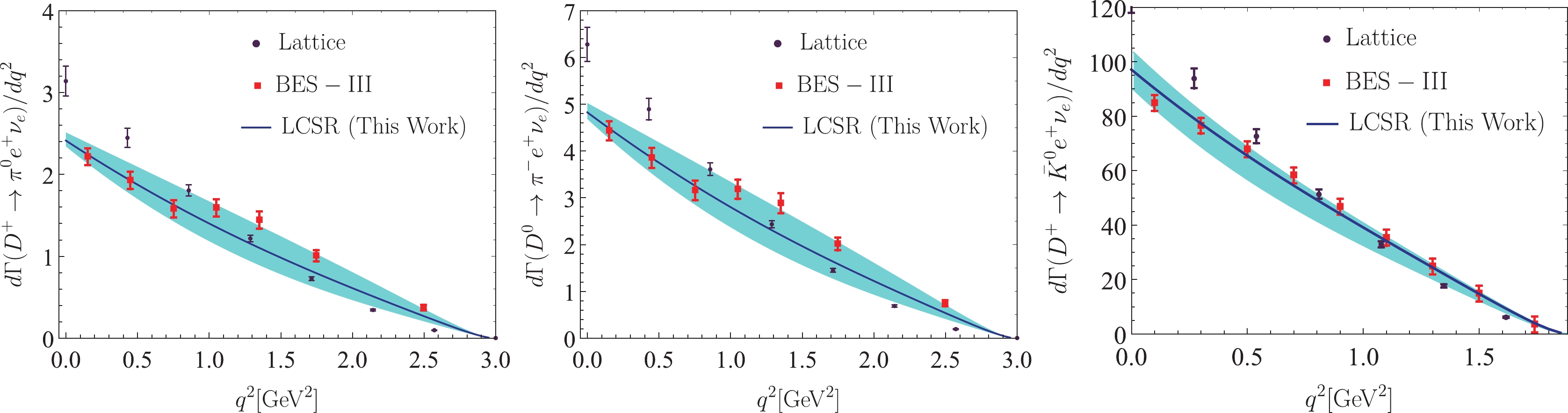
As a further step, the branching fractions of
$ D\to P \ell^+ \nu_\ell $ can be obtained by employing$ \tau({D^0}) = 0.410(2)\; {\rm{ps}} $ and$ \tau({D^+}) = 1.040(7)\; {\rm{ps}} $ and integrating with the squared momentum transfer, the results are presented in Table 6. The relevant experimental results, BES-III [15], CLEO-c [8], PDG [54], Belle [7], BABAR [9], and theoretical results of the covariant quark model (CQM) [62] are also presented for comparison. Our results on the branching fractions for$ D\to \pi \ell^+ \bar\nu_\ell $ and$ D\to K \ell^+ \bar\nu_\ell $ are consistent with the BES-III measurements within error limits. Compared with the CQM theoretical predictions for the$ D^+\to \pi^0\ell^+\nu_\ell $ channel, our results are closer to the experimental results.Channel LCSR(This Work) BES-III [15] CLEO-c [8] BABAR [9] Belle [7] PDG [54] CQM [62] $ { D^+\to\bar K^0e^+\nu_e}$ 

$ { 8.547^{+0.445}_{-1.108}}$ 

8.60(6)(15) 8.83(10)(20) − − − 8.84 $ { D^+\to\bar K^0\mu^+\nu_\mu}$ 

$ { 8.435^{+0.437}_{-1.100}}$ 

8.72(7)(18) − − − − 8.60 $ { D^+\to\pi^0e^+\nu_e}$ 

$ { 0.328^{+0.056}_{-0.044}}$ 

0.36(8)(5) 0.405(16)(9) − − − 0.309 $ { D^+\to\pi^0\mu^+\nu_\mu}$ 

$ { 0.325^{+0.056}_{-0.044}}$ 

− − − − − 0.303 $ { D^0\to K^-e^+\nu_e}$ 

$ { 3.370^{+0.176}_{-0.437}}$ 

3.505(14)(33) 3.50(3)(4) − 3.45(7)(20) 3.538(33) 3.46 $ { D^0\to K^-\mu^+\nu_\mu}$ 

$ { 3.325^{+0.172}_{-0.433}}$ 

3.505(14)(33) − − − 3.33(13) 3.36 $ { D^0\to \pi^-e^+\nu_e}$ 

$ { 0.258^{+0.044}_{-0.035}}$ 

0.295(4)(3) 0.288(8)(3) 0.277(7)(9) 0.255(19)(16) − 0.239 $ { D^0\to \pi^-\mu^+\nu_\mu}$ 

$ { 0.256^{+0.044}_{-0.035}}$ 

− − − − 0.238(24) 0.235 Table 6. Branching fractions of
$D\to P\ell^+\nu_\ell$ (in unit$10^{-2}$ ). The errors are squared averages of all the mentioned error sources. For comparison, we also present the prediction of various methods.Furthermore, the ratios for branching fractions for different lepton channels are defined as,
$ R_P = {\Gamma(D\to P\mu^+\nu_\mu)}/{\Gamma(D\to P e^+\nu_e)}. $ After inputting the$ D\to P\ell^+\nu_\ell $ decay width into the above equation and replacing HFFs with Eqs. (16) and (17), we can get ratios of semileptonic fractions as follows:$ \begin{split} & R_{\pi^0} = \frac{\Gamma(D^+ \to \pi^0 \mu^+\nu_\mu)}{\Gamma(D^+ \to \pi^0 e^+\nu_e)} = 0.991^{+0.230}_{-0.197},\\ & R_{\pi^-} = \frac{\Gamma(D^0 \to \pi^- \mu^+\nu_\mu)}{\Gamma(D^0 \to \pi^- e^+\nu_e)} = 0.992^{+0.231}_{-0.198}, \\ & R_{\bar K^0} = \frac{\Gamma(D^+ \to \bar K^0 \mu^+\nu_\mu)}{\Gamma(D^+ \to \bar K^0 e^+\nu_e)} = 0.987^{+0.156}_{-0.138},\\ & R_{K^-} = \frac{\Gamma(D^0 \to K^- \mu^+\nu_\mu)}{\Gamma(D^0 \to K^- e^+\nu_e)} = 0.987^{+0.156}_{-0.138}. \end{split}$

(34) The above ratios from our calculations are consistent with the CQM prediction
$ R_{\bar K^0}^{\rm{CQM}} = 0.97 $ [62], which is very close to$ 1 $ .Moreover, the obtained HFFs can be used to calculate the forward-backward asymmetry
$ {\cal{A}}_{\rm{FB}}(q^2) $ , which can be expressed as follows:$ {\cal{A}}_{\rm{FB}}^\ell(q^2) = \frac{3\delta_\ell{\cal{P}}_0^P (q^2) {\cal{P}}_t^P(q^2)} {(1+\delta_\ell)|{\cal{P}}_0^P(q^2) |^2+3|{\cal{P}}_t^P(q^2) |^2} . $

(35) Further, the lepton side convexity parameter
$ {\cal{C}}_F^\ell(q^2) $ can be written as:$ {\cal{C}}_F^\ell(q^2) = -\frac32\frac{(1-2\delta_\ell)|{\cal{P}}_0^P(q^2) |^2}{(1+\delta_\ell)|{\cal{P}}_0^P(q^2) |^2+3\delta_\ell|{\cal{P}}_t^P(q^2) |^2}.$

(36) After inputting the HFFs into Eqs. (35) and (36), we present the forward-backward asymmetry and the lepton convexity parameter within uncertainties in Fig. 3. Finally, we list the mean values for forward-backward asymmetry
$ \langle{\cal{A}}_{\rm{FB}}^\ell\rangle $ and lepton convexity parameter$ \langle{\cal{C}}_F^\ell\rangle $ in Table 7. It is seen that for both$ D\to \pi\ell\bar\nu_\ell $ and$ D\to K\ell\bar\nu_\ell $ decay transitions,$ \langle{\cal{A}}_{\rm{FB}}^\mu\rangle $ is approximately$ 10^5 $ times larger than$ \langle{\cal{A}}_{\rm{FB}}^e\rangle $ , while$ \langle{\cal{C}}_F^\mu\rangle $ is slightly larger than$ \langle{\cal{C}}_F^e\rangle $ . For$ D\to P\ell\nu_\ell $ , our predictions are different from the CQM results [62]. Considering that the formulas in Eqs. (35) and (36) refer to HFFs, these differences may provide a way to test those HFFs in future experiments.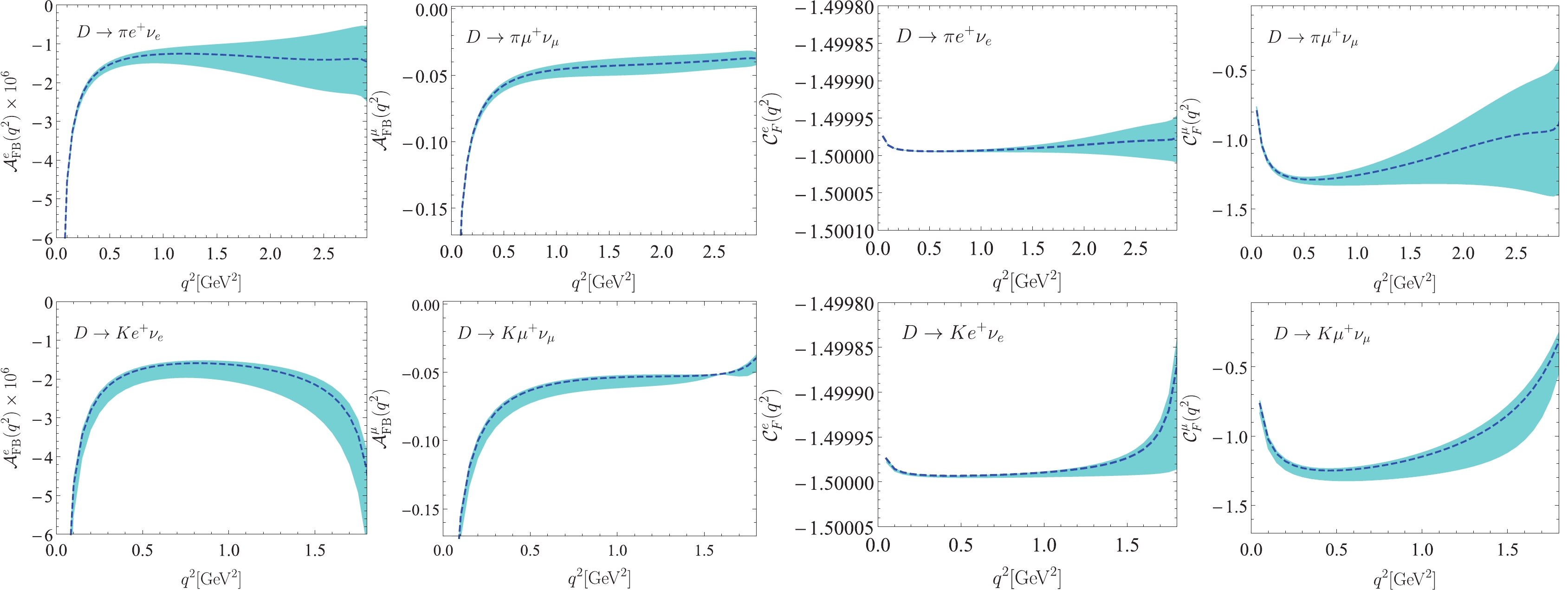
Figure 3. (color online) Forward-backward asymmetries and the convexity parameters of the decays
$ D\to\pi\ell^+\nu_\ell $ and$ D\to K\ell^+\nu_\ell $ with$ \ell = e, \mu $ ; the shaded bands correspond to the uncertainties from the theoretical input parameters.Channel $ { \langle{\cal{A}}_{\rm{FB}}^\ell\rangle}$ (This work)

$ { \langle{\cal{C}}_F^\ell\rangle}$ (This work)

$ { \langle{\cal{A}}_{\rm{FB}}^\ell\rangle}$ (CQM) [62]

$ { \langle{\cal{C}}_F^\ell\rangle}$ (CQM) [62]

$ { D\to\pi e^+\nu_e}$ 

$ { \big(-4.827^{+0.947}_{-1.247}\big)\times 10^{-6}}$ 

$ { -4.425^{+0.000}_{-0.000}}$ 

$ { -4.1\times 10^{-6}}$ 

$ { -1.5}$ 

$ { D\to\pi\mu^+\nu_\mu}$ 

$ { -0.155^{+0.013}_{-0.017}}$ 

$ { -3.303^{+0.396}_{-0.509}}$ 

$ { -0.04}$ 

$ { -1.37}$ 

$ { D\to K e^+\nu_e}$ 

$ { \big(-4.564^{+0.316}_{-1.310}\big)\times 10^{-6}}$ 

$ { -2.775^{+0.000}_{-0.000}}$ 

$ { -4.27\times 10^{-6}}$ 

$ { -1.5}$ 

$ { D\to K \mu^+\nu_\mu}$ 

$ { -0.123^{+0.003}_{-0.015}}$ 

$ { -1.866^{+0.063}_{-0.274}}$ 

−0.058 −1.32 Table 7. Forward-backward asymmetry and lepton convexity parameter. The errors are squared averages from all the mentioned error sources.
-
In this study, we investigated the
$ D \to P $ HFFs$ {\cal{P}}_\sigma^P (q^2) $ with$ \sigma = 0,t $ within the LCSR approach up to NLO gluon radiation correction for twist-2 contributions accuracy. At large recoil point$ q^2 \rightsquigarrow 0\; {{\rm{GeV}}^2} $ , we have$ {\cal{P}}_{t,0}^\pi(0) = 0.688^{+0.020}_{-0.024} $ and$ {\cal{P}}_{t,0}^K(0) = 0.780^{+0.024}_{-0.029} $ . The detailed uncertainties of these predictions caused by the errors in the input parameters are given in Table 3. Then, contributions of the LO and NLO to the LCSR results are given in Table 4, and the maximal contribution of NLO for$ {\cal{P}}_{0,t}^P(0) $ is no more than 3%. These results indicate that the HFFs maintain a high-accuracy and our predictions, which are based on it, are credible.After extrapolating the
$ D\to P $ HFFs to the whole physical$ q^2 $ -region, the behavior of these HFFs within uncertainties was depicted in Fig 1. Furthermore, we applied these HFFs to study the semilepton decay processes$ D\to P\ell\nu_\ell $ . For the decay width in Fig. 2, our results agreed with the BES-III collaboration within error limits, especially in the low$ q^2 $ regions. Using the D-meson lifetime, we obtained the two types of branching ratios and listed them in Table 6. Our predictions are in good agreement with the BES-III and other experimental results, providing a better prediction of the$ D\to \pi \ell\nu_\ell $ decay process than that of the CQM [62]. Meanwhile, we listed the ratios of branching fractions with different lepton channels$ R_P $ in Eq. (34), which showed that$ R_{\bar K^0} = R_{K^-} $ and all values of these ratios are close to 1.As a further step, by taking the
$ D\to P $ HFFs into the forward-backward asymmetry$ {\cal{A}}_{\rm{FB}}^\ell(q^2) $ and the lepton convexity parameter$ {\cal{C}}_F^\ell(q^2) $ , we plot these two observables in Fig. 3. Meanwhile, the mean values for the forward-backward asymmetry$ \langle{\cal{A}}_{\rm{FB}}^\ell\rangle $ and lepton convexity parameter$ \langle{\cal{C}}_F^\ell\rangle $ are listed in Table 7. The table shows that$ \langle{\cal{A}}_{\rm{FB}}^\mu\rangle $ are approximately$ 10^5 $ times larger than$ \langle{\cal{A}}_{\rm{FB}}^e\rangle $ . There is a considerable difference between our result and the CQM for both$ \langle{\cal{A}}_{\rm{FB}}^\ell\rangle $ and$ \langle{\cal{C}}_F^\ell\rangle $ for the$ D\to P \ell\nu_\ell $ decay. This discrepancy may provide a way to test those HFFs in future experiments.We are grateful to Prof. Xing-Gang Wu and Tao Zhong for many helpful discussions and suggestions.
D → P(π, K) helicity form factors within light-cone sum rule approach
- Received Date: 2020-05-05
- Available Online: 2020-11-01
Abstract: In this study,


 DownLoad: