-
Since the recent discovery from type Ia supernova data [1-3] that our universe has been expanding at an accelerated rate, many dark energy models have been proposed to explain these phenomena [4-9]. The simplest one is the
$ \Lambda{\rm{CDM}} $ model, in which$ \Lambda $ represents the cosmological constant term. However,$ \Lambda{\rm{CDM}} $ encounters some difficulties, primarily the "fine tuning" [10,11] and "coincidence" [12-14] problems.The running vacuum model (RVM) [15,16] has been introduced to solve the "coincidence problem", where the cosmological constant term is assumed to vary with the Hubble parameter
$ H $ . This model links the existence of dark energy to the theoretical mechanism of the quantum field, which may trigger the primordial inflation scenario [17], and fits with the observational data better than$ \Lambda{\rm{CDM}} $ [18]. In the literature, the spatially flat RVM has been extensively investigated [18-35].Recently, the Planck Legacy 2018 analysis by Valentino, Melchiorri, and Silk in Ref. [36] has suggested that the universe is closed at 99% C.L. [37]. Similar conclusions have been obtained by Park and Ratra in the context of non-spatially-flat DE models [38-41]. Nevertheless, when the BAO data set is included together with the CMB, the evidence in favor of a non-spatially-flat universe disappears completely [36,42,43]. These interesting results encourage us to study RVM in a non-flat universe [44,45], in addition to a flat one [18]. With the involvement of non-zero spatial curvature, it is inevitable to encounter degeneracies between the curvature and other parameters. One of them is the famous "geometrical degeneracy" [46,47] in CMB power spectra, caused by different sets of parameters that lead to the same value of the angular diameter distance of the last scattering. Conversely, when fitting with observational data, the non-zero spatial curvature also broadens the constraints of the cosmological parameters [48].
In this work, we concentrate on the running cosmological constant in the non-flat universe,
$ \Lambda = 3\nu (H^{2}+ K/a^2)+c_0 $ , where$ \nu $ and$ c_{0} $ are the model parameters,$ a $ represents the scalar factor, and$ K $ corresponds to the spatial curvature constant. We first study the CMB power spectra in this non-flat RVM and discuss the degeneracy between$ \nu $ and the density parameter of curvature$ \Omega_K = -K/(aH)^2 $ . We then constrain the cosmological parameters of both non-flat RVM and$ \Lambda{\rm{CDM}} $ with the observational data using the Markov chain Monte Carlo (MCMC) method, and we compare the results with those in the flat universe. The effectiveness of RVM versus$ \Lambda{\rm{CDM}} $ in the non-flat universe is also tested based on the minimal$ \chi^2 $ values.This paper is organized as follows. In Sec. 2, we introduce the non-flat RVM and derive the background evolution equations. We compare the CMB power spectra of RVM in the non-flat universe along with the Planck 2018 data and show the constraints of the cosmological parameters in Sec. 3. Our conclusions are presented in Sec. 4.
-
We start with the Einstein field equation of the RVM, given by
$ R_{\alpha\beta}-\frac{1}{2} g_{\alpha\beta} R+g_{\alpha\beta} \Lambda = \kappa^2 T_{\alpha\beta}, $

(1) where
$ \kappa^2 = 8\pi G $ is set to 1 for simplicity,$ R = g^{\alpha\beta}R_{\alpha\beta} $ represents the Ricci scalar,$ T_{\alpha\beta} $ stands for the energy-momentum tensor for matter and radiation, and$ \Lambda $ corresponds to the dynamical cosmological constant.The spatially isotropic and homogeneous universe can be described by the Robertson-Walker metric:
$ {\rm d}s^{2} = -{\rm d}t^{2}+a^2(t)\left\{\frac{{\rm d}r^2}{1-Kr^2} +r^2 {\rm d}\theta^2+r^2\sin^2\theta {\rm d}\phi^2 \right\}\,, $

(2) where
$ a $ is the scale factor, while$ K $ is a constant describing the spatial curvature, with$ K = 1,0,-1 $ corresponding to closed, flat, and open universes, respectively. Then, the Friedmann equations can be expressed as$ H^{2} = \frac{1}{3}(\rho_m + \rho_r + \rho_{\Lambda})-\frac{K}{a^2} \,, $

(3) $ \dot{H} = - \frac{1}{2} (\rho_m + \rho_r + \rho_{\Lambda} + P_m+ P_r + P_{\Lambda})+\frac{K}{a^2}, \, $

(4) where
$ \rho_{m, r, \Lambda} $ ($ P_{m, r, \Lambda} $ ) are the energy densities (pressures) of matter, radiation, and dark energy, respectively, and$H = {\rm d}a/(a{\rm d}t)$ represents the Hubble parameter. We note that$ \rho_{\Lambda} = \kappa^{-2} \Lambda $ , and the density parameters are given by$ \Omega_{m, r} = \frac{\rho_{m, r}}{3H^2} , $

(5) $ \Omega_{\Lambda} = \frac{\Lambda}{3H^2} , $

(6) $ \Omega_K = -\frac{K}{a^2 H^2}. \, $

(7) In the non-flat universe, the running cosmological constant term is set to
$ \Lambda = 3\nu H^{2}+3\nu \frac{K}{a^2}+c_0\,, $

(8) where
$ \nu $ is a non-negative model parameter to ensure that the energy density of dark energy is positive in the early universe;$ c_0 $ is given by$ c_0 = -3\nu ( H_0^2+K)+\Lambda_0 $ , where$ H_0 $ and$ \Lambda_0 $ are the values of the Hubble parameter and cosmological constant, respectively. The model becomes$ \Lambda{\rm{CDM}} $ when$ \nu = 0 $ . The corresponding equations of state in this model can be defined as$ w_{m, r, \Lambda} = \frac{P_{m, r, \Lambda}}{\rho_{m, r, \Lambda}} = 0, \frac{1}{3}, -1 \,. $

(9) For the energy transformations from dark energy to matter and radiation, the modified continuity equations are given by
$ \dot{\rho}_{m, r}+3 H(1+w_{m, r})\rho_{m, r} = Q_{m, r} \,, $

(10) $ \dot{\rho}_\Lambda+3 H(1+w_\Lambda)\rho_\Lambda = - Q \,, $

(11) with
$ Q_{m}+Q_{r} = Q $ ,$ Q_{m, r} $ can be written as$ Q_{m, r} = -\frac{\dot{\rho}_{\Lambda}(\rho_{m, r}+P_{m, r})}{\rho_{m}+\rho_{r}+P_m+P_r} = 3\nu H(1+w_{m, r})\rho_{m, r}\,. $

(12) By combining Eqs. (3)-(12), we derive the energy densities as functions of the scale factor:
$ \rho_{m}(a) = \rho_{m}^{(0)}a^{-3\xi} , $

(13) $ \rho_{r}(a) = \rho_{r}^{(0)}a^{-4\xi} , $

(14) $ \rho_{\Lambda}(a) = \rho_{\Lambda}^{(0)}+\left(\xi^{-1}-1\right)\left [\rho_m^{(0)}\left(a^{-3\xi}-1\right)+\rho_r^{(0)}\left(a^{-4\xi}-1\right)\right] , $

(15) where
$ \rho_{m,r.\Lambda}^{(0)} $ are current values and$ \xi = (1-\nu) $ . Consequently, the Friedmann equation defined in Eq. (3) can be rewritten as$ H^{2} \!=\! H_{0}^{2}\left\{\frac{1}{\xi}\left[\Omega_{m}^{0}\left(a^{-3\xi}\!-\!1\right)+\Omega_{r}^{0}\left(a^{-4\xi}\!-\!1\right)\right]+\Omega_{K}^{0}\left(a^{-2}\!-\!1\right)\!+\!1\right\} , $

(16) where
$ \Omega_{m,r,K}^{0} $ are current values of density parameters. -
To study the degeneracy between the cosmological parameters, we first modify the CAMB [49] program to generate theoretical CMB power spectra for both the RVM and
$ \Lambda{\rm{CDM}} $ . The results are presented in Sec. 3.1. We then use the CosmoMC package [50], which is a Markov Chain Monte Carlo (MCMC) engine exploring the cosmological parameter space, to constrain RVM and$ \Lambda{\rm{CDM}} $ from the observational data. For simplification, we use$ \Omega_K $ afterward to represent the density parameter of curvature at the present time, except where specifically indicated. -
There is "geometrical degeneracy" between the curvature and other parameters in the CMB power spectra. To see this effect, we compare the CMB power spectra of RVM and
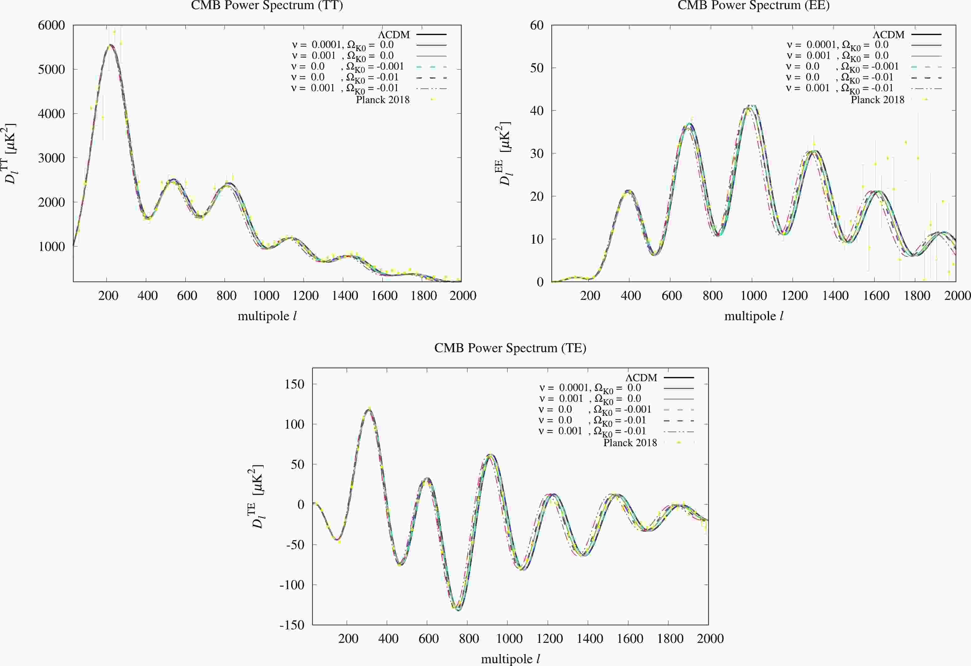
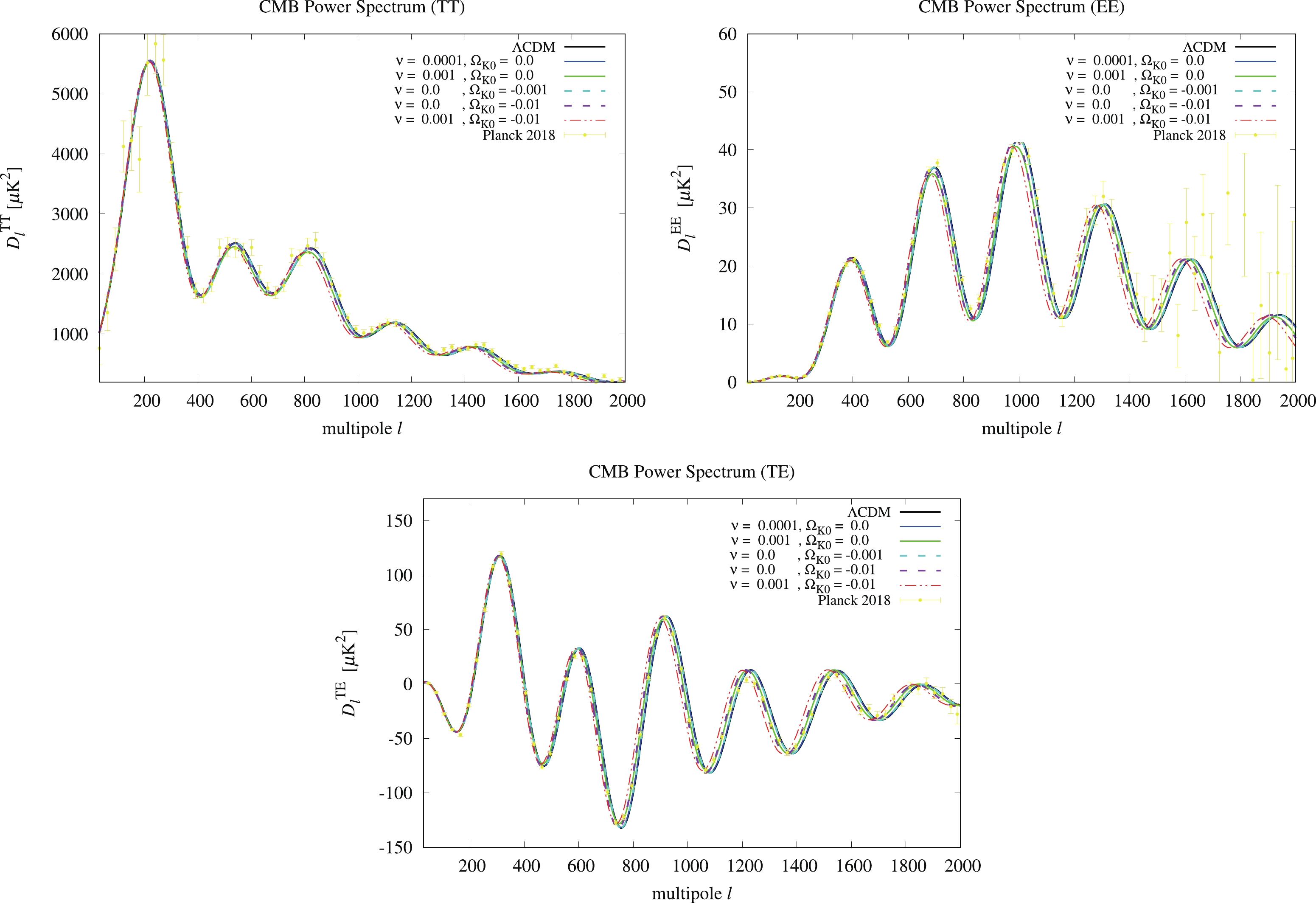
$ \Lambda{\rm{CDM}} $ with various values of$ \nu $ and$ \Omega_K $ along with the observational data from Planck 2018 [43]. From previous studies [18,33,34] with$ 0 \leqslant \nu \leqslant O(10^{-3}) $ in RVM for the flat universe and the result of$ -0.007 \geqslant \Omega_K \geqslant -0.095 $ at 99% C.L. in Ref. [36], we choose$ 0 \leqslant \nu < 0.01 $ and$ 0 \geqslant \Omega_K \geqslant -0.01 $ to see the degeneracy between$ \nu $ and$ \Omega_K $ in the CMB power spectra. Furthermore, the$ \Lambda{\rm{CDM}} $ model is recovered when$ \nu = 0 $ and$ \Omega_K = 0 $ in Eq. (8).In Fig. 1, we present the CMB power spectra for the TT, EE, and TE modes from the CAMB package. It can be seen that
$ 0\leqslant\nu\leqslant O(10^{-3}) $ (solid lines) and$ 0 \geqslant \Omega_K \geqslant -O(10^{-2}) $ (dashed lines) fit well with the data from Planck 2018. The residues with respect to$ \Lambda{\rm{CDM}} $ are plotted in Fig. 2. We find that the geometrical degeneracy with$ (\nu, \Omega_K) = (0.001,0) $ (green solid line) and$ (0.0, -0.01) $ (purple dashed line) has similar results in the CMB power spectra. However, only$ \nu $ can cause strong suppression of the TT mode spectra when$ \nu > 0 $ . In addition, the effects of$ \nu $ and$ K $ show an additive property in the CMB power spectra (red dash-dotted line). -
To constrain the cosmological parameters of RVM and
$ \Lambda{\rm{CDM}} $ in the non-flat universe, we use the CosmoMC package with an MCMC engine to explore the parameter space with combinations of the observational data sets, which include the CMB temperature fluctuation from Planck 2018 with TT, TE, EE, low-$ l $ polarization from SMICA [43,51-53], BAO data from the 6dF Galaxy Survey [54] and BOSS [55], supernova (SN) data from the JLA compilation [56], the weak lensing (WL) data from CFHTLenS [57] and direct large-scale structure (LSS) formation data, and the data points of$ f\sigma_8 $ listed in Table 1. The priors of parameters are given in Table 2. Because of the tension between the geometry data (SNIa, BAO, etc.) and growth data (WL,$ f\sigma_8 $ ) [74], we choose the two combinations CMB+BAO+SN and CMB+BAO+SN+WL+$ f\sigma_8 $ in our fits. To calculate the best fitted values of$ \chi^2 $ , we use$ z $ 

$ f\sigma_8 $ 

Ref. $ z $ 

$ f\sigma_8 $ 

Ref. $ z $ 

$ f\sigma_8 $ 

Ref. $ 1 $ 

$ 1.36 $ 

$ 0.482 \pm 0.116 $ 

[58] $ 10 $ 

$ 0.59 $ 

$ 0.488 \pm 0.06 $ 

[66] $ 19 $ 

$ 0.35 $ 

$ 0.440 \pm 0.05 $ 

[61,69] $ 2 $ 

$ 0.8 $ 

$ 0.470 \pm 0.08 $ 

[59] $ 11 $ 

$ 0.57 $ 

$ 0.444 \pm 0.038 $ 

[67] $ 20 $ 

$ 0.32 $ 

$ 0.394 \pm 0.062 $ 

[67] $ 3 $ 

$ 0.78 $ 

$ 0.38 \pm 0.04 $ 

[60] $ 12 $ 

$ 0.51 $ 

$ 0.452 \pm 0.057 $ 

[64] $ 21 $ 

$ 0.3 $ 

$ 0.407 \pm 0.055 $ 

[65] $ 4 $ 

$ 0.77 $ 

$ 0.490 \pm 0.18 $ 

[61,62] $ 13 $ 

$ 0.5 $ 

$ 0.427 \pm 0.043 $ 

[65] $ 22 $ 

$ 0.25 $ 

$ 0.351 \pm 0.058 $ 

[68] $ 5 $ 

$ 0.73 $ 

$ 0.437 \pm 0.072 $ 

[63] $ 14 $ 

$ 0.44 $ 

$ 0.413 \pm 0.080 $ 

[63] $ 23 $ 

$ 0.22 $ 

$ 0.42 \pm 0.07 $ 

[60] $ 6 $ 

$ 0.61 $ 

$ 0.457 \pm 0.052 $ 

[64] $ 15 $ 

$ 0.41 $ 

$ 0.45 \pm 0.04 $ 

[60] $ 24 $ 

$ 0.17 $ 

$ 0.51 \pm 0.06 $ 

[61,70] $ 7 $ 

$ 0.60 $ 

$ 0.390 \pm 0.063 $ 

[63] $ 16 $ 

$ 0.4 $ 

$ 0.419 \pm 0.041 $ 

[65] $ 25 $ 

$ 0.15 $ 

$ 0.49 \pm 0.15 $ 

[71] $ 8 $ 

$ 0.6 $ 

$ 0.433 \pm 0.067 $ 

[65] $ 17 $ 

$ 0.38 $ 

$ 0.430 \pm 0.054 $ 

[64] $ 26 $ 

$ 0.067 $ 

$ 0.423 \pm 0.055 $ 

[72] $ 9 $ 

$ 0.60 $ 

$ 0.43 \pm 0.04 $ 

[60] $ 18 $ 

$ 0.37 $ 

$ 0.460 \pm 0.038 $ 

[68] $ 27 $ 

$ 0.02 $ 

$ 0.36 \pm 0.04 $ 

[73] Table 1. Data points of
$ f\sigma_8 $ .Parameter Prior RVM parameter $ \nu $ 

$ 0.0 \leqslant \nu \leqslant 3.0\times10^{-4} $ 

Curvature parameter $ \Omega_K $ 

$ -0.25 \leqslant \Omega_K \leqslant 0.2 $ 

Baryon density $ 0.5 \leqslant 100\Omega_bh^2 \leqslant 10 $ 

CDM density $ 0.1 \leqslant 100\Omega_ch^2 \leqslant 99 $ 

Optical depth $ 0.01 \leqslant \tau \leqslant 0.8 $ 

Neutrino mass sum $ 0 \leqslant \Sigma m_{\nu} \leqslant 2 $ eV

$ \dfrac{\mathrm{Sound \; horizon}}{\mathrm{Angular \; diameter \; distance}} $ 

$ 0.5 \leqslant 100 \theta_{MC} \leqslant 10 $ 

Scalar power spectrum amplitude $ 2 \leqslant \ln \left( 10^{10} A_s \right) \leqslant 4 $ 

Spectral index $ 0.8 \leqslant n_s \leqslant 1.2 $ 

Table 2. Priors for cosmological parameters with the non-flat RVM of
$ \Lambda = 3\nu (H^{2}+ K/a^2)+c_0 $ .$ \chi^2_c = \sum\limits_{i = 1}^n \frac{(T_c(z_i) - O_c(z_i))^2}{E^i_c} \,, $

(17) where
$ c $ denotes the type of the data,$ n $ is the number of the data in each data set,$ T_c $ represents the theoretical value derived from CAMB at redshift$ z_i $ , and$ O_c $ ($ E_c $ ) corresponds to the observational value (covariance).The global fitting results of RVM and
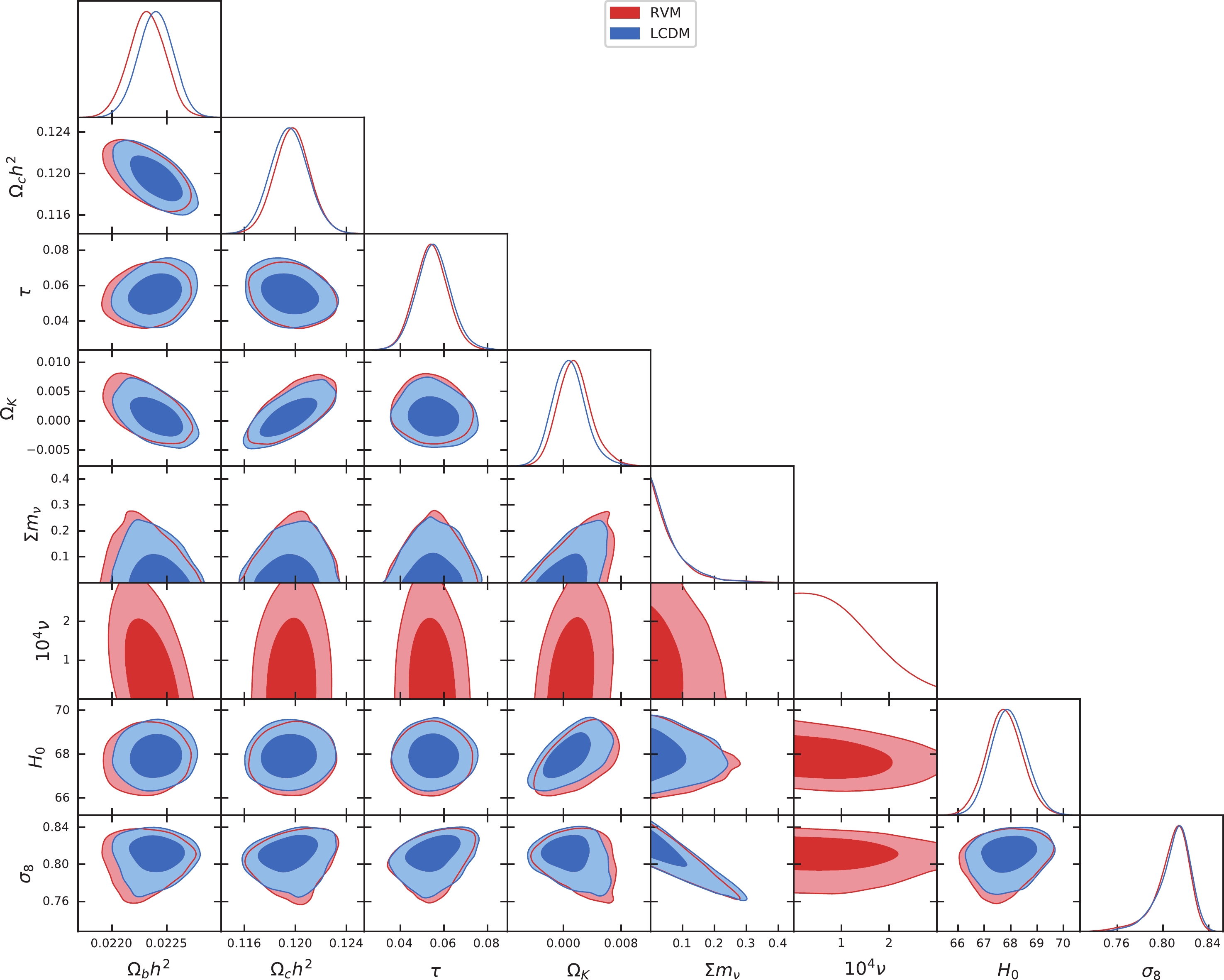
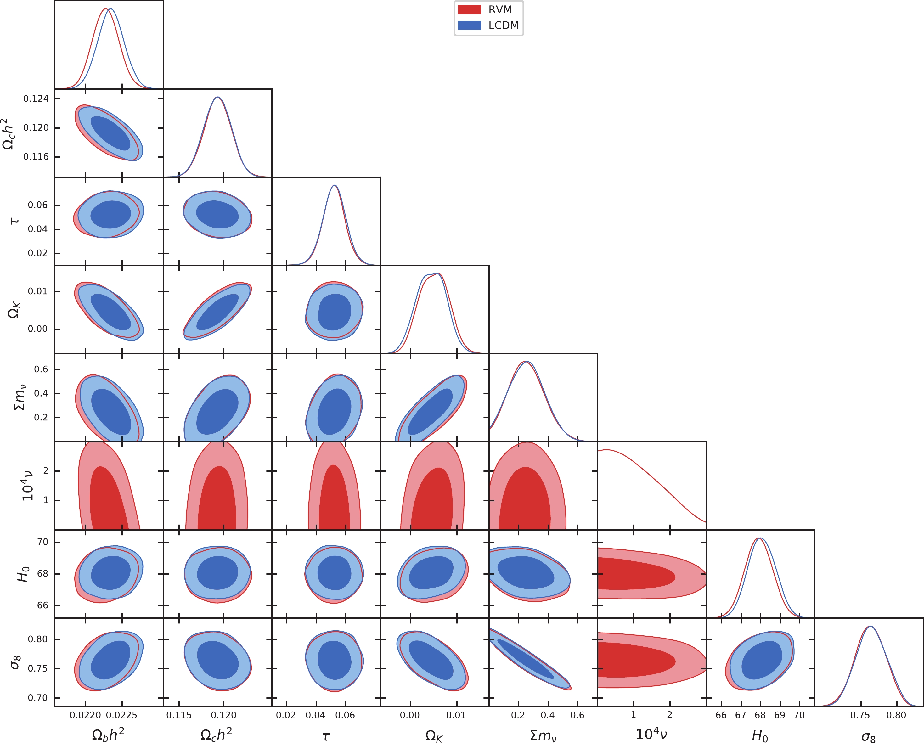
$ \Lambda{\rm{CDM}} $ in the non-flat universe are plotted in Figs. 3 and 4, while those listed in Table 3 correspond to the cosmological parameters and$ \nu $ , given at 95% and 68% C.L., respectively. Our results show that$ \nu\lesssim 1.39 \times10^{-4} $ at 68% C.L. in the non-flat universe of RVM for the data set CMB+BAO+ SN+WL+$ f\sigma_8 $ , which is similar to the previous result of$ 1.54\times10^{-4} $ at 68% C.L. in RVM for a flat universe [33]. Explicitly, we obtain that$\chi^2_{\rm RVM} = 3472.32\; (3523.74)$ and$\chi^2_{\Lambda\rm CDM} = 3474.92\; (3524.51)$ when fitting with the data set CMB+BAO+SN (CMB+BAO+SN+WL+$ f\sigma_8 $ ), indicating that our results in RVM are consistent with those in$ \Lambda{\rm{CDM}} $ for a non-flat universe. For the density parameter$ \Omega_K $ of the spatial curvature at the present time, our results show that an open universe is preferred, instead of the closed one in Ref. [36]. In particular, when the data of WL and$ f\sigma_8 $ are included, both RVM and$ \Lambda{\rm{CDM}} $ favor an open universe with$ |\Omega_K|\leqslant O(10^{-2}) $ . Our result for the open universe is consistent with that in Ref. [75].
Figure 3. (color online) One- and two-dimensional distributions of
$ \Omega_b h^2 $ ,$ \Omega_c h^2 $ ,$ \tau $ ,$ \Omega_K $ ,$ \sum m_\nu $ ,$ 10^4 \nu $ ,$ H_0 $ , and$ \sigma_8 $ for RVM and$ \Lambda{\rm{CDM}} $ in a non-flat universe with the combined data CMB+BAO+SN, where the contour lines represent 68% and 95% C.L., respectively.Parameter CMB+BAO+SN CMB+BAO+SN+WL+ $f\sigma_8$ 

Model RVM $\Lambda{\rm{CDM}}$ 

RVM $\Lambda{\rm{CDM}}$ 

${\bf{100\Omega_b h^2}}$ 

$2.23 \pm 0.03 $ 

$2.24 \pm 0.03 $ 

$2.23^{+0.04}_{-0.03}$ 

$2.23 \pm 0.04$ 

${\bf{100\Omega_c h^2}}$ 

$12.0 \pm 0.3 $ 

$12.0 \pm 0.3 $ 

$11.9 \pm 0.3 $ 

$11.9 \pm 0.3 $ 

${\bf{100\tau}}$ 

$5.43^{+1.52}_{-1.45}$ 

$5.53^{+1.62}_{-1.52}$ 

$5.22^{+1.56}_{-1.50}$ 

$5.23^{+1.54}_{-1.58}$ 

${\bf{10^3\Omega_K}}$ 

$1.55^{+4.91}_{-4.54}$ 

$0.80^{+4.72}_{-4.53}$ 

$5.10^{+5.97}_{-5.94}$ 

$4.53^{+5.92}_{-5.99}$ 

${\bf{\Sigma m_\nu}}$ [eV]

$<0.199$ 

$<0.188$ 

$0.256^{+0.224}_{-0.234}$ 

$0.257^{+0.219}_{-0.234}$ 

${\bf{10^4 \nu}}$ 

$<1.36$ 

$-$ 

$<1.39$ 

$-$ 

$H_0$ [km/s/Mpc]

$67.8^{+1.4}_{-1.3}$ 

$67.9^{+1.3}_{-1.2}$ 

$67.9^\pm 1.4$ 

$68.1^{+1.4}_{-1.3}$ 

$\sigma_8$ 

$0.808^{+0.027}_{-0.034}$ 

$0.810^{+0.026}_{-0.031}$ 

$0.764^{+0.040}_{-0.042}$ 

$0.765\pm 0.040$ 

$\chi^2_{\rm best\text{-}fit}$ 

$3472.32$ 

$3474.92$ 

$3523.74$ 

$3524.51$ 

Table 3. Fitting results for RVM and
$ \Lambda{\rm{CDM}} $ in a non-flat universe, where the cosmological parameters and$ \nu $ are given at 95% and 68% C.L., respectively.
Figure 4. (color online) One- and two-dimensional distributions of
$ \Omega_b h^2 $ ,$ \Omega_c h^2 $ ,$ \tau $ ,$ \Omega_K $ ,$ \sum m_\nu $ ,$ 10^4 \nu $ ,$ H_0 $ , and$ \sigma_8 $ for RVM and$ \Lambda $ CDM in a non-flat universe with the combined data CMB+BAO+SN+WL+$ f\sigma_8 $ , where the contour lines represent 68% and 95% C.L., respectively.The best-fit values of the neutrino mass sum,
$ \Sigma m_{\nu} $ , in a non-flat universe are similar to those in a flat universe when fitting with CMB+BAO+SN [18,76-78]. However, it is interesting to see that the constraints on$ \Sigma m_{\nu} $ are relaxed for the data set CMB+BAO+SN+WL+$ f\sigma_8 $ , in which the$ f\sigma_8 $ data points play the main role. Note that similar results are also obtained in a flat universe, as shown in Ref. [18]. This is because the structure-growth rate of$ f\sigma_8 $ is a unique indicator of massive neutrinos [79,80]. Specifically, we have$ \Sigma m_{\nu} = 0.256^{+0.224}_{-0.234} $ ($ 0.257^{+0.219}_{-0.234} $ ) eV at 95% C.L., resulting in non-zero lower bounds of$ \Sigma m_{\nu} \geqslant 0.022\; (0.023) $ eV at 95% C.L. for RVM ($ \Lambda{\rm{CDM}} $ ) in a spatially curved universe. Conversely, becuase of the possible degeneracy among$ \tau $ ,$ \Omega_K $ , and$ \Sigma m_{\nu} $ , the constraints on$ \tau $ and$ \Omega_K $ are not improved with the data points of WL+$ f\sigma_8 $ , as seen from Table 3. To obtain better constraints, some additional data could be used, such as$21\;{\rm cm}$ emission measurements [81,82], which could fix the parameter$ \tau $ to break the degeneracy of$ \tau $ ,$ \Omega_K $ , and$ \Sigma m_{\nu} $ [79,80]. We note that in our data fitting, we do not specify the neutrino mass hierarchy in$ \Sigma m_\nu $ . For the cosmological effects of the neutrino mass hierarchy, refer to the discussion in the literature [83-85]. -
We have studied the running vacuum model with a cosmological constant of
$ \Lambda = 3\nu (H^{2}+ K/a^2)+c_0 $ in a spatially curved universe. We have compared our results for several sets of$ \nu $ and$ \Omega_K $ with the Planck 2018 data in the CMB power spectra. We have found that$ \nu $ and$ \Omega_K $ have similar effects on the CMB power spectra, but only non-zero values of$ \nu $ lead to large suppressions in the CMB TT mode spectra. In the two combinations of the observational data, we have constrained$ \nu \leqslant O(10^{-4}) $ , together with$ |\Omega_K|\leqslant O(10^{-2}) $ . Notably, the constraints on$ \nu $ in a non-flat universe are similar to those in a flat universe. From the best fitted values of$ \chi^2 $ , we have shown that RVM is inconsistent with$ \Lambda{\rm{CDM}} $ . When fitting with the data set CMB+BAO+SN+WL+$ f\sigma_8 $ , we have obtained non-zero lower bounds of$ \Sigma m_{\nu} \geqslant 0.022 $ and 0.023 eV at 95% C.L. in the non-flat RVM and$ \Lambda{\rm{CDM}} $ , respectively, indicating that the involvement of a non-zero$ \Omega_K $ can provide viable constraints on the absolute neutrino masses in cosmological models.K. Z. would like to thank Dr. Yangsheng Yuan and Shandong Normal University for part of the numerical calculations run by the workstation of their group.
Running vacuum model in a non-flat universe
- Received Date: 2020-03-19
- Accepted Date: 2020-06-07
- Available Online: 2020-10-01
Abstract: We investigate observational constraints on the running vacuum model (RVM) of


 Abstract
 HTML
HTML Reference
 Related
 PDF
PDF


 DownLoad: