Quantum ekpyrotic mechanism in Fermi-bounce curvaton cosmology

Andrea Addazi; Antonino Marciano

doi:10.1088/1674-1137/aba58d

Chinese Physics C> 2020, Vol. 44> Issue(10) : 105101 DOI: 10.1088/1674-1137/aba58d

Quantum ekpyrotic mechanism in Fermi-bounce curvaton cosmology

Center for Field Theory and Particle Physics & Department of Physics, Fudan University, Shanghai 200433, China

Abstract
HTML
Reference
Related

PDF

Abstract：
Within the context of the Fermi-bounce curvaton mechanism, we analyze the one-loop radiative corrections to the four-fermion interaction, generated by the non-dynamical torsion field in the Einstein-Cartan-Holst-Sciama-Kibble theory. We show that contributions that arise from the one-loop radiative corrections modify the energy-momentum tensor, mimicking an effective Ekpyrotic fluid contribution. Therefore, we call this effect quantum Ekpyrotic mechanism. This leads to the dynamical washing out of anisotropic contributions to the energy-momentum tensor, without introducing any new extra Ekpyrotic fluid. We discuss the stability of the bouncing mechanism and derive the renormalization group flow of the dimensional coupling constant ξ, checking whether any change of its sign takes place towards the bounce. This enforces the theoretical motivations in favor of the torsion curvaton bounce cosmology as an alternative candidate to the inflation paradigm.
- bounce cosmology ,
- fermion bounce ,
- ekpyrotic bounce ,
- non-dynamical torsion

1. Introduction

1. Introduction
2. Theory
3. Matter bounce and ekpyrosis
     3.1 Bouncing models
     3.2 Ekpyrotic models
4. One-loop corrections
     Lowest n-point contributions
     $2n$ -point contributions
5. RG flow and stability
6. Conclusions
Appendix
     Appendix A: The $4$ -function at $1$ -loop
     Appendix B: The $2n$ -function at $1$ -loop

The cosmological bounce scenario, as originated by standard model matter fields, is a viable alternative to inflation that has not yet been ruled out experimentally. The concept of the bounce is that the cosmological dynamics emerges from a pre-Big Bang universe, which solves the cosmological singularity. Almost scale-invariant perturbations are generated during the (matter) contracting cosmological phase — see e.g. Ref. [1] — thus satisfying CMB observations [2]. A scale-invariant power spectrum can be also recovered for curvature perturbations in a matter-filled emergent universe, as in [3]. A possible origin of the bounce can be recovered within the context of the Einstein-Cartan-Holst-Sciama-Kibble theory (ECHSK) [4-7], accounting for gravity with a topological Holst term and non-minimally coupled fermions. In the first-order formalism, one must allow for a torsionful part of the spin-connection, as gravity is coupled to fermion fields. In this framework, the torsion field does entail propagating degrees of freedom and can be integrated-out as an auxiliary field. By virtue of the torsion-fermion coupling, new effective four-fermion interactions arise. A sort of effective Nambu-Jona-Lasinio (NJL) model can emerge, but from a very different dynamical origin than the one addressed in the QCD case. Depending on the sign of the fermion-torsion coupling, this can provide a new attractive or repulsive contribution to the energy conditions. In the repulsive phase, with a certain choice of the torsion-fermion coupling, such a term can contribute to the energy-momentum tensor, triggering a bounce at a related critical energy density scale. Possible bounce cosmology scenarios were investigated in Refs. [8-11]. A detailed analysis of the phenomenological consequences, at late cosmological times, of theories with fermions that violate the Null Energy Condition (NEC) was provided in [12].

A typical issue for bounce scenarios in cosmology is the generation of large $O(1)$ anisotropic terms in the energy-momentum tensor, which is incompatible with the cosmological isotropy of the CMB. An approach to solve this problem requires the introduction of a new exotic fluid, the Ekpyrotic fluid, provided with an energy-density steeply scaling with the Universe scale factor, i.e. $\rho_{\rm{Ek}} = \rho_{0}a^{-n}$ with $n>6$ . The Ekpyrotic fluid does dominate during the Bounce critical scale, suppressing anisotropic contributions to the background dynamics. However, both the classical Bounce and the Ekpyrotic mechanism are based on a classical analysis. During the Bounce stage, quantum corrections are expected to be large, and potentially they may completely change and wash-out the Bounce dynamics, along with the Ekpyrotic classical solution to the anisotropies' problem.

This highly motivates the analysis of quantum corrections to the Ekpyrotic mechanism in some specific Bounce cosmology models. In this study, we analyze the one-loop quantum corrections to the four-fermion term generated by torsion, in a Friedmann-Lemaître-Robertson-Walker (FLRW) background. We show that quantum corrections induce extra corrections to the classical bare energy-momentum, which was previously not considered. We find that these new radiative terms theoretically have two healthy consequences: $i)$ they favor the classical Bounce, generating contributions that violate the NEC; $ii)$ they generate new terms mimicking the effect of the Ekpyrotic fluid. This result implies that the four-fermion curvaton mechanism can induce the Bounce without introducing any new exotic matter field. This hypothesis is theoretically appealing, as it avoids adding any particle to the theoretical framework that cannot be accommodated in the Standard Model of particle physics, or in any Grand Unified extensions of it.

2. Theory

1. Introduction
2. Theory
3. Matter bounce and ekpyrosis
     3.1 Bouncing models
     3.2 Ekpyrotic models
4. One-loop corrections
     Lowest n-point contributions
     $2n$ -point contributions
5. RG flow and stability
6. Conclusions
Appendix
     Appendix A: The $4$ -function at $1$ -loop
     Appendix B: The $2n$ -function at $1$ -loop

We follow the theoretical framework and the conventions introduced in Refs. [4-21]. This makes us consider a generalization of the Einstein-Hilbert action with a topological term, the Holst action for gravity in the Palatini formalism, which allows to couple gravity to chiral fermions. The theory can be coupled to a Dirac field $\psi$ , and to the related field $\overline{\psi} = \left(\psi^{*}\right)^{T}\gamma^{0}$ . The Dirac action involves the Dirac matrices, $\gamma^I$ with $I = 0,\cdots,3$ and $\gamma^5$ . The action for pure gravity can be cast in terms of the gravitational field $g_{\mu \nu} = e_{\mu}^I e_{\nu}^J \eta_{IJ}$ , where $e^I_\mu$ is the tetrad/frame field (with inverse $e_I^\mu$ and determinant e), and the Lorentz connection $\omega^{IJ}_\mu$ . The curvature of $\omega^{IJ}_\mu$ , namely

$F^{I J}_{\mu\nu} = 2 \partial_{[\mu}\omega^{IJ}_{\,\nu]} + \left[ \omega_\mu, \omega_\nu \right]^{IJ}\,,$

is the triadic projection of the Riemann tensor.

The total action involves the Einstein-Cartan-Holst (ECH) action — namely the Palatini-formulated action for gravity plus fermions that also includes the topological term à la Holst, which resembles the $\theta$ -term for gauge fields — with a non-minimal component of the covariant Dirac action. Note that, in absence of the gravitational Holst topological term, the whole theory provided with torsion and minimally-coupled fermions is referred to in the literature as the Einstein-Cartan-Sciama-Kibble theory (see e.g. Refs. [4-6]). In the Palatini first order formalism, the ECH action casts (see e.g. [11]),

${S}_{\rm{Holst}} = \dfrac{1}{2 \kappa} \int_{M}\!\! {\rm d}^{4}x \;|e| \, e^{\mu}_{I}e^{\nu}_{J} P^{IJ}_{\ \ \ KL}F^{\ \ KL}_{\mu \nu}(\omega)\,.$

(1)

In Eq. (1), $\kappa = 8 \pi G_{\rm{N}}$ is the square of the reduced Planck length, $\epsilon_{IJKL}$ denotes the Levi-Civita symbol, while the tensor in the internal indices $P^{IJ}_{\ \ \ KL} = \delta^{[I}_{K} \delta^{J]}_{L} - \epsilon^{IJ}_{\ \ KL}/ (2 \gamma)$ involves the Barbero–Immirzi parameter $\gamma$ and is invertible for $\gamma^2\neq -1$ . The Dirac action for massless fermions reads $S_{\rm{Dirac}} = \!\dfrac{1}{2 } \int {\rm d}^{4}x |e| {\cal{L}}_{\rm{Dirac}}$ , with

${\cal{L}}_{\rm{Dirac}} = \!\dfrac{\imath}{2 } \overline{\psi}\!\left(1-\dfrac{\imath}{\alpha}\gamma_{5}\right)\!\gamma^{I}e^{\mu}_{I} \nabla_{\mu}\psi + {\rm{h.c.}} \, .$

(2)

In Eq. (2), $\alpha$ denotes a real parameter called non-minimal coupling. For $\alpha\! = \!\gamma$ , we may recover the Einstein-Cartan action, namely $S_{\rm{ECH}}\!\! = \!\!S_{\rm{GR}} \!+\! S_{\rm{Dirac}}$ . An additional term is also present, which reduces to the Nieh-Yan invariant (see e.g. Ref. [20]) when the second Cartan structure equation is satisfied. Within the framework of the Holst action in Eq. (1), the minimal coupling can be recovered in the limit $\alpha \rightarrow \pm\infty$ . Phenomenologically allowed values of the parameters $\alpha$ and $\gamma$ are recovered from the four fermion axial-current Lagrangian (7), from measurements of lepton-quark contact interactions [14, 22].

The presence of fermions induces a torsional part of the connection to enter the non-minimal ECH action. Torsion is non-dynamical in this theory, and can be integrated out once the second Cartan structure equation is solved. This requires to introduce the contortion tensor $C_\mu^{IJ}$ , which is defined by $(\nabla_\mu-\widetilde{\nabla}_\mu ) V_I = C_{\mu \,I}^{\ \ J}\, V_J\,,$ with $\widetilde{\nabla}_\mu$ denoting the covariant derivative compatible with the tetrad $e^I_\mu$ and $V_J$ a vector in the internal space. The Cartan equation expresses the contortion tensor $C_\mu^{IJ}$ in terms of the fermions' currents and the tetrad, namely

$\begin{split} & e^\mu_I \, C_{\mu JK} = \dfrac{\kappa}{4} \, \dfrac{\gamma}{\gamma^2 +1} \, \left( \beta \, \epsilon _{IJKL}\ J^L - 2 \theta \, \eta_{I[J} \, J_{K]} \right) \,, \\ &J^L = \overline{\psi} \gamma^L \gamma_5 \psi \, . \end{split}$

(3)

The coefficients appearing in Eq. (3) are related to the free parameters of the non-minimal ECH theory, $\beta = \gamma+1/\alpha$ and $\theta = 1-\gamma/\alpha$ . Deploying the solution in (3), the non-minimal ECH action recasts in terms only of the metric compatible variables, further including a novel interaction term that captures the new physics:

$S_{\rm{ECH}} = S_{\rm{GR}} + S_{\rm{Dirac}} +S_{\rm{Int}}\,.$

(4)

In Eq. (4), the Einstein-Hilbert action involves the mixed-indices Riemann tensor $R_{\mu\nu}^{IJ} = F_{\mu\nu}^{IJ}[\widetilde{\omega}(e)]$ , namely

$S_{GR} = \dfrac{1}{2 \kappa} \int_{M} \!\!\! {\rm d}^4 x |e| e^\mu_I e^\nu_J R_{\mu\nu}^{IJ} \,,$

(5)

the Dirac action $S_{\rm{Dirac}}$ on curved space-time recasts in terms of the metric compatible variables

$S_{\rm{Dirac}} = \dfrac{\imath}{2} \int_{M} \!\!\! {\rm d}^4 x |e| \ \overline{\psi} \gamma^I e^\mu_I \widetilde{\nabla}_\mu \psi +{\rm{h.c.}}\,,$

(6)

while the interacting term reads

$S_{\rm{Int}} \! = \! -\xi \kappa\! \int_{M} \!\!\! {\rm d}^4 x |e| \,J^L\, J^M\, \eta_{LM}\,,$

(7)

with the coefficient $\xi$ being a function of the fundamental parameters of the theory, namely

$\xi: = \dfrac{3}{16} \!\dfrac{\gamma^2}{\gamma^2+1}\! \left(1 + \dfrac{2}{\alpha \gamma} - \dfrac{1}{\alpha^2} \right)\,.$

(8)

In few words, the net effect of having coupled fermions to gravity in the first order formalism means to have recovered, in the metric-compatible formalism, an extra four fermion term. That means that the structure of General Relativity remains untouched, but that the matter part of the Einstein equations acquires at tree-level a self-interaction term, the coupling constant of which, $\xi$ , can be either positive or negative. Furthermore, we shall comment that the choice of real values of $\gamma$ , which allows to retain only real-valued effective potentials, ensures that the reality condition is automatically implemented on the gravitational field.

For completeness, we show in this section the energy-momentum tensor components, i.e.

$T^{\rm{fer}}_{\mu\nu}\! = \! \dfrac{1}{4} \overline{\psi} \gamma_I e^I_{( \mu} \imath \widetilde{\nabla}_{\nu )} \psi +{\rm{h.c.}} - g_{\mu\nu} {\cal{L}}_{\rm{fer}}\,.$

(9)

3. Matter bounce and ekpyrosis

1. Introduction
2. Theory
3. Matter bounce and ekpyrosis
     3.1 Bouncing models
     3.2 Ekpyrotic models
4. One-loop corrections
     Lowest n-point contributions
     $2n$ -point contributions
5. RG flow and stability
6. Conclusions
Appendix
     Appendix A: The $4$ -function at $1$ -loop
     Appendix B: The $2n$ -function at $1$ -loop

Only a complete treatment of the vast literature that hinges on the matter bounce scenario would require per se a sizable review. For the purpose of our analysis, we will devote this section to provide an introductory review of the argument, focusing on the cases of scalar matter fields, and then of fermion fields. Then, we will summarize a few crucial elements of the ekpyrotic models, in preparation for our analysis and the discussion of the novelty of our framework.

It is rather important also to emphasize that matter bounce cosmologies may achieve a nearly scale-invariant power spectrum, and they are characterized by a slightly red tilt of the scalar perturbations and a small tensor-to-scalar ratio. Furthermore, a positive running of the scalar index may provide in this scenario few distinctive predictions, an enlightening element to be kept in mind, as it distinguishes from the scenario our analysis hinges on, and the predictions that arise in one-field inflation and ekpyrotic models [23]. Thus, this paradigm provides the concrete chance to falsify a matter bounce scenario with forthcoming observations.

3.1 Bouncing models

1. Introduction
2. Theory
3. Matter bounce and ekpyrosis
     3.1 Bouncing models
     3.2 Ekpyrotic models
4. One-loop corrections
     Lowest n-point contributions
     $2n$ -point contributions
5. RG flow and stability
6. Conclusions
Appendix
     Appendix A: The $4$ -function at $1$ -loop
     Appendix B: The $2n$ -function at $1$ -loop

A bounce scenario can be achieved either by modifying in an effective way the Einstein equations, or by assuming a matter field content that violates the null energy conditions (NEC). We can revive the main directions along which the bounce scenario is attained, fitting them into the following classes:

● String Cosmology:

a resolution of the Big Bang singularity is notably provided by string theory, through the picture of a gas of strings that evolve in a space-time with compactified dimensions on a circle of radius R — specifically, one should deal with weakly coupled ${\cal{N}} = (4,0)$ superstrings compactified to 4D. The thermal properties of the gas should then explain the emergence of a bounce. The one-loop partition function $Z(R)$ is finite and fulfills thermal duality (dubbed T-duality)

$Z(R) = Z\left( \dfrac{R_c^2}{R} \right)\,,$

(10)

with $R_c$ being of the order of the string length [24]. At the critical point $R\! = \!R_c$ , thermal string states start to become massless and to condensate. For time-dependent temperatures, the time-slices on which the condensates appear form space-like branes, or S-branes. As a byproduct of T duality, and of the formation of the string condensate, a maximal temperature $T_{\rm{max}}$ is reached at the critical point. Thus, the string gas cools both for $R\!>\!\!>\!R_c$ , a regime where the energy of the strings is mostly concentrated in their momentum, and $R\!<\!\!<\!R_c$ , a regime where the energy of the strings is concentrated in windings around compactified dimensions. Therefore, one can imagine a process for which the string gas starts at a cold temperature, in the winding regime, and then gradually increases, until it reaches $T_{\rm{max}}$ , at which a phase transition takes place to the momentum regime. Hence, the temperature starts to decrease again. The thermodynamical properties of the string gas then imply the dynamical features of the cosmological evolution. The conservation of the thermal entropy of matter fields in a co-moving volume (in four-dimensional homogeneous space-time), which reads

$S = a^3 \, \dfrac{\rho +p }{T} \sim (aT)^3\,,$

(11)

with a scale factor and p pressure density, then implies that $a\, T$ is constant. A bouncing cosmology follows, in which T increases until it reaches the maximal value $T_{\rm{max}}$ , and then decreases again. At the same time, the scale factor a decreases until it reaches a minimal value, for $T\! = \!T_{\rm{max}}$ , at which a bounce of the universe happens. Perturbation of the action at second order around the FLRW solution enables to compute the evolution of the cosmological perturbations from the pre-bounce contracting phase. This was achieved for instance in [25], due to the presence of the S-brane at the bounce instantiating a transition toward the expanding post-bounce phase.

● Loop Quantum Cosmology (LQC):

a theory inspired and motivated by the non-perturbative quantization methods of Loop Quantum Gravity [26] is Loop Quantum Cosmology (LQC) [27]. Within this framework, a bounce picture [28] emerges at a critical Planckian energy density $\rho_{\rm{c}}\simeq \rho_{\rm{Pl}}$ , which determines the energy scale of the bounce, namely

$H^2 = \dfrac{8 \pi G}{3} \rho \left(1-\dfrac{\rho}{\rho_{\rm{c}}} \right)\,,$

(12)

H denoting the Hubble parameter. In this picture, the continuity equation is not deformed by the curvature scale. For perturbations that can be described as long-wavelength Fourier modes, the separate universe approximation [29] applies, and the effective Friedmann equations in each patch provides the usual form of the long-wavelength Mukhanov-Sasaki equation.

● $f(R)$ and extended gravity:

modified gravity theories that belong to the class of $f(R)$ extension of the Einstein-Hilbert action, defined by the action

$S = \dfrac{1}{2\kappa} \int {\rm d}^4x \sqrt{-g}\, f(R) \,,$

(13)

have been invoked either to explain dark matter and/or dark energy, or to provide a consistent ultraviolet completed theory of quantum gravity, with higher order curvature terms in the action that become relevant when approaching the Planck scale [30]. Furthermore, $f(R)$ gravity allows to mimic several bouncing scenarios. Specifically, a change of variables allows to unveil the dynamics of $f(R)$ theories: for

$g_{\mu \nu} \rightarrow \tilde{g}_{\mu \nu} = f' g_{\mu \nu} = \phi \, g_{\mu \nu},$

(14)

and

$\phi\rightarrow \tilde{\phi}\,, \quad {\rm{with}} \quad {\rm d}\tilde{\phi} = \sqrt{\dfrac{3}{2\kappa}}\, \dfrac{{\rm d}\phi}{\phi}\,,$

(15)

the theory recasts

$S = \int {\rm d}^4x \sqrt{-g} \left[ \dfrac{\tilde{R}}{2 \kappa} -\dfrac{1}{2} (\partial \tilde{\phi})^2 - U(\tilde{\phi}) \right]\,,$

(16)

with $U(\tilde{\phi}) = (Rf'-f)/(2\kappa {f'}^2)$ . This enables an analysis of the cosmological perturbations over the pre-bounce phase, as affected by $f(R)$ theories.

● Effective Field theory:

As a violation of NEC, effective field theory scenarios have been also envisaged to achieve bouncing cosmologies. A particular instantiation can be provided by ghost condensates scalar fields, which are employed to generate the bounce [31-34]. Introducing both a Horndeski-type operator and a dynamical ghost condensate operator, non-singular bounce cosmological models can be obtained, with a Lagrangian expressed in the Kinetic Gravity Braiding (KGB) form by

$L\! = \!K(\phi,X)+ G(X),$

(17)

$K(\phi,X)\! = \![1-g(\phi)] X +\dfrac{\beta X^2}{M_{\rm{Pl}}^4} -V(\phi)\,,$

(18)

$G(X)\! = \!\dfrac{\gamma X}{M_{\rm{Pl}}^3}\,,$

(19)

where $X = g^{\mu \nu} (\partial_\mu \phi )(\partial_\nu \phi )/2$ is the regular kinetic term for the scalar field $\phi$ , $\beta$ , and $\gamma$ are real-valued parameters, $g(\phi)$ is a function of the scalar field, and $g^{\mu \nu} \nabla_\mu \nabla_\nu$ d'Alembertian operator, with $\nabla_\mu$ as the gravitational covariant derivative. As soon as for (even for a short time) $g(\phi)\!>\!\!>\!1$ , ghost condensation phase starts, giving rise to a non-singular bounce. For $\beta>0$ , the $\beta X^2$ term stabilizes at high energy scales the kinetic energy.

● Fermi Bounce:

Both the non-minimal ECH and the ECHSK actions entail of four-fermion term that can trigger the instantiation of a matter bounce. This term, corresponding to a fermionic superconductive scenario, directly originates from torsion. Nonetheless, effective higher order operators can be phenomenologically introduced, as in [35], even if fermions are coupled to gravity cast in a metric compatible form. For a fermion of mass m, one can consider a potential of the form

$V(\bar{\psi} \psi) = V_0+ m \bar{\psi}\psi - \lambda (\bar{\psi}\psi )^2\,,$

(20)

with $V_0$ contribution to the cosmological constant and $\lambda$ a dimensionfull coupling constant. For positive values of $\lambda$ , the fermion system can induce a bounce scenario. Cosmic evolution can be studied resorting to a time-reversed description of the expanding universe. One can start considering the epoch over which matter energy density dominates over the fermion energy density, but the latter is still positive. Because for an expanding universe $\bar{\psi} \psi \propto 1/a^{3}$ , over reversed time direction the value of the fermion bilinear increases, and the fermion energy density becomes negative, while the other form of energy density, due to radiation ( $\propto a^{-4}$ ) and dust ( $\propto 1/a^{3}$ ), redshift away and approach zero. A bounce then takes place when the negative fermion energy density equals in absolute value the sum of the other matter energy density contributions.

● Quintom bounce:

The Quintom scenario intertwines among the quintessence and the phantom paradigms, combined into a unique scenario for dark energy. Within this framework, the system is characterized by a dynamically evolving equation of state $p\! = \!w\rho$ , which crosses over the cosmic evolution the critical value $w\! = \!-1$ , corresponding to the cosmological constant. The phases along which the system evolves are characterized by a phantom-energy-like behavior when $w\!<\!-1$ , and by a quintessence-like behavior for $w\!>\! -1$ .

As shown in [36], quintom models entailing dark energy that deal with ideal gases and scalar fields, requires the presence of at least two degrees of freedom, as summarized in the Lagrangian

$L = \dfrac{1}{2} \partial_\mu \phi \partial^\mu \phi - \partial_\mu \varphi \partial^\mu \varphi - V(\phi, \varphi)\,,$

(21)

where potential can be specialized to have the Coleman-Weinberg form

$V(\phi, \varphi) = \dfrac{1}{4} \lambda \phi^4 \left(\ln \dfrac{|\phi|}{v}-\dfrac{1}{4} \right) +\dfrac{1}{16}\lambda v^4\,,$

(22)

as in [37]. In contrast, a quintom model involving a fermion field was studied in [12]. The decay of the quintom energy may then trigger avoidance of the Big Bang and Big Rip singularity. Specifically, Quintom models for inflation can be constructed, as in [37], in which the bounce replaces the Big Bang singularity [38].

Below, we address a specific model of bouncing cosmology, to encompass the elements that are necessary to a direct comparison with the results we are about to derive.

3.2 Ekpyrotic models

1. Introduction
2. Theory
3. Matter bounce and ekpyrosis
     3.1 Bouncing models
     3.2 Ekpyrotic models
4. One-loop corrections
     Lowest n-point contributions
     $2n$ -point contributions
5. RG flow and stability
6. Conclusions
Appendix
     Appendix A: The $4$ -function at $1$ -loop
     Appendix B: The $2n$ -function at $1$ -loop

Ekpyrotic cosmologies appeared within the framework of string theory, such as to allow a bounce interconnecting the Big Crunch and Big Bang singularities. Singularities correspond here to brane collisions in higher-dimensions [39-41]. This is thus a viable realization of the matter cosmological bounce scenario.

The basic ingredients of the most straightforward version of the ekpyrotic scenario coincide with those ones of inflation, i.e., a scalar field rolling down a potential $V(\phi)$ . However, as opposed to inflation, here the potential is steep and negative. This is a crucial feature that induces a slower contraction than inflation. Indeed, instead of an exponentially growing scale factor and a corresponding almost constant Hubble radius, which set a quasi de Sitter geometry, in this scenario the scale factor is almost constant, and the Hubble radius rapidly shrinks, a situation that corresponds to an approximately flat space-time.

The ekpyrotic potential is generically composed by three parts:

1. a steep and negative part, down which the potential rolls with sizable kinetic energy, providing a scaling solution with attractor. Over this phase, the large-scale density fluctuations are generated once the modes of the perturbed field exit the horizon. The so-called fast-roll conditions hold, namely

$\epsilon \equiv \dfrac{1}{M_{\rm{Pl}}} \left( \dfrac{V}{V_{,\,\phi}} \right)^2\!\!<\!\!<1 \,, \!\!\quad \!\! \eta \equiv 1\!-\! \dfrac{V_{,\,\phi \phi} V}{V^2_{,\,\phi}} \!\!<\!\!<1 \,.$

(23)

Usually, an approximated potential that satisfies these conditions is

$V(\phi)\simeq - V_0 \exp \left( - \sqrt{\dfrac{2}{k}} \dfrac{\phi}{M_{\rm{Pl}}} \right) \,,$

(24)

in which k is a real parameter that satisfies $k<\!\!<1$ . The scaling behavior then ceases as soon as (23) are no-longer valid;

2. to avoid that a large negative vacuum energy is left, at the end of the ekpyrotic phase one usually assumes that the potential has a minimum, thus rising it back up to positive values;

3. a further part is left unconstrained by the specific features of the ekpyrotic scenario.

On a Friedmann-Lemaître-Robertson-Walker (FLRW) spacetime, specified in comoving coordinates by

${\rm d}s^2 = -{\rm d}t^2 +a^2 {\rm d}{{x}}\cdot {\rm d}{{x}}\,,$

(25)

with $a = a(t)$ scale factor, the first Friedmann equation and the evolution of the scalar field read, respectively,

$3 H^2 \, M^2_{\rm{Pl}} \! = \! \dfrac{1}{2} \dot{\phi}^2 +V(\phi)\,,$

(26)

$\ddot{\phi} + 3 H \dot{\phi} \! = \! - V_{,\,\phi} \,.$

(27)

Specifying the potential as in (24), a scaling solution is found:

$a(t) \sim (-t)^k\,, \qquad H = \dfrac{k}{t} \,;$

(28)

$\phi(t) = \sqrt{2k} \, M_{\rm{Pl}} \,\ln \left( - \sqrt{\dfrac{V_0}{M^2_{Pl} \, k(1-3k)} } \, t \right)\,.$

(29)

At $k<\!\!<1$ , the scalar field entails large values of both the kinetic and the potential energy term. Nonetheless, the resulting total energy density is small, since the two contributions almost cancel. Furthermore, the scaling solution is an attractor and retains the equation of state of a very stiff fluid, with

$w = p/\rho = 2/(3 k) -1 >\!\!>1\,.$

(30)

This is a very remarkable property, as it entails that $\rho_{\phi}\sim a^{-2/k}$ , which for $k<\!\!<1$ implies a more relevant blueshift than any other contribution to the Friedmann equation, either curvature ( $\sim \! a^{-2}$ ), or matter ( $\sim \! a^{-3}$ ), or radiation ( $\sim \! a^{-4}$ ), or anisotropy ( $\sim \! a^{-6}$ ). Thus, this term will be predominant with respect to anisotropies, while approaching the bounce.

4. One-loop corrections

1. Introduction
2. Theory
3. Matter bounce and ekpyrosis
     3.1 Bouncing models
     3.2 Ekpyrotic models
4. One-loop corrections
     Lowest n-point contributions
     $2n$ -point contributions
5. RG flow and stability
6. Conclusions
Appendix
     Appendix A: The $4$ -function at $1$ -loop
     Appendix B: The $2n$ -function at $1$ -loop

Because non-dynamical torsion provides an interaction term, we may reconstruct at one-loop the quantum effective action of the matter part of the theory. For simplicity, to calculate the these terms, we assume the background to be FLRW, which in conformal coordinates reads

${\rm d}s^{2} = a^{2}(-{\rm d}\eta^{2}+{\rm d}{ x}\cdot {\rm d}{ x})\,,$

(31)

with $a = a(\eta)$ scale factor and $\eta$ conformal time.

The four-fermion vertex is

${\cal{V}}_{4} = -\imath \, {\xi} \kappa\, \gamma_{\mu}\gamma_{5} \otimes \gamma^{\mu}\gamma_{5}.$

(32)

The massless Feynman propagator — for a detailed analysis involving massive fermions, we refer to Refs. [22, 42] — in position space between the points x and $\tilde{x}$ is denoted as $\imath S_{F}(x,\tilde{x})$ , and reads

$\imath S_{F}(x,\tilde{x}) = (a\tilde{a})^{-\frac{D-1}{2}} \dfrac{\Gamma(D/2-1)}{4 \pi^{D/2}}\, \imath \gamma^a \partial_a\, \dfrac{1}{\Delta x_{++}^{D-2}(x,\tilde{x})}\,,$

(33)

having denoted $\tilde{a} = a(\tilde{\eta})$ , and

$\Delta x_{++}^{D-2}(x,\tilde{x}) = ( \left\Vert {{x}}-{\tilde{{x}}}\right\Vert ^{2}-\left|\eta-\tilde{\eta}\right|^{2})^{D-2}\,,$

(34)

in which the two spacetime points are labelled with $x = \{\eta, {{x}} \}$ and $\tilde{x} = \{\tilde{\eta}, \tilde{{{x}}} \}$ . Eq. (33) is anstraightforward result to be calculated, which is easier than the estimate of the massless scalar propagator, because of the conformal nature of massless fermions in any dimension — see e.g. [43, 44]. Assuming fermion matter content to be massless around the bounce is a viable approximation, given that the critical energy density at bounce is considerably above the condensate phase of the Higgs. In this preliminary study, we disregard to include Yukawa couplings of fermionic species to the Higgs, leaving a refined analysis to a forthcoming analysis [45].

The sign of the coupling constant $\xi$ , expressed in Eq. (8) in terms of the bare parameters of the ECHSK theory, $\alpha$ and $\gamma$ , individuates two phases at the cosmological level. For $\xi>0$ , the theory is in a Fermi liquid phase, with a tree-level repulsive interaction that has been studied as a source of dark energy [21], or to drive inflation [46]. Instead, the super-conductive phase corresponds to the branch of values $\xi<0$ , for which a bouncing scenario has been taken into account [10, 11, 13, 15, 16, 35]. Therefore, we will proceed taking into account negative values of $\xi$ in what follows. In Sec. 5, we come back to the issue of the quantum stability of the bounce, and analyze the running of the $\xi$ parameter around the bounce.

Lowest n-point contributions

1. Introduction
2. Theory
3. Matter bounce and ekpyrosis
     3.1 Bouncing models
     3.2 Ekpyrotic models
4. One-loop corrections
     Lowest n-point contributions
     $2n$ -point contributions
5. RG flow and stability
6. Conclusions
Appendix
     Appendix A: The $4$ -function at $1$ -loop
     Appendix B: The $2n$ -function at $1$ -loop

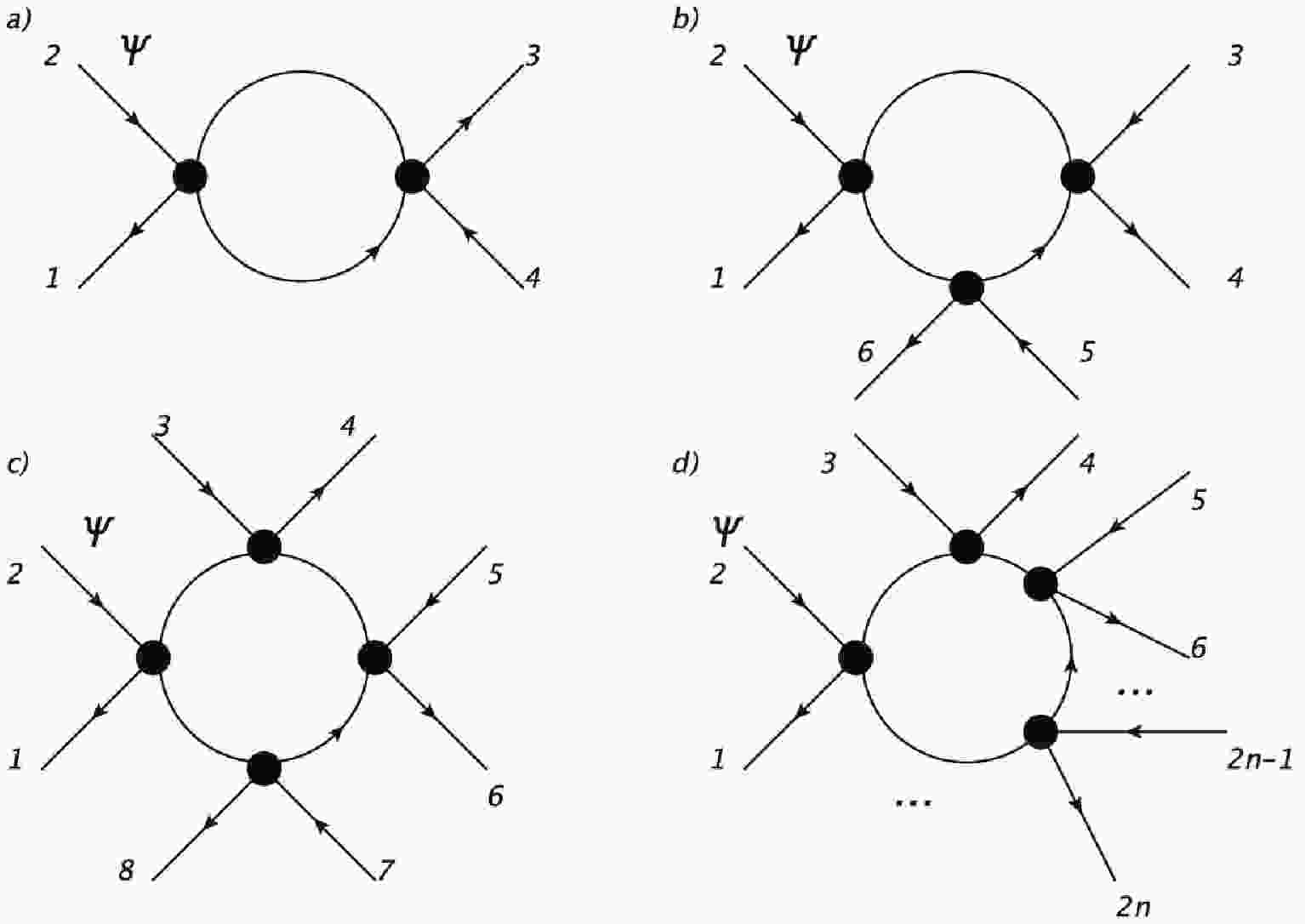
We start considering the 2-point and the 3-point 1-loop contributions to the effective action, derived from the evaluation of the diagrams in Fig. 1a and Fig. 1b. For the former one, derived from the Wick contraction of two pairs of axial currents, one has to calculate the tensorial contribution $\Pi^{\mu \nu}_{2}$ , which is defined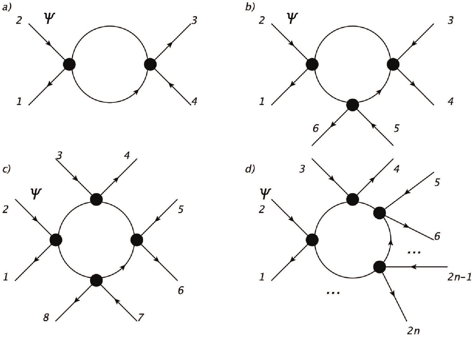

Figure 1

Figure 1. a) One-loop correction to the four-fermions self-interaction term; b) one loop correction to the six-points self-interaction term; c) one loop correction to the eight-points self-interaction term; d) one loop correction to the 2n-points self-interaction term.

DownLoad: Full-Size Img PowerPoint

$\Pi_{2}^{\mu \nu} = -{\rm{Tr}}_{x'} [ \gamma^\mu \gamma^5 S_{F}(x,\tilde{x}) \gamma^\nu \gamma^5 S_{F}(\tilde{x},x)]\,,$

(35)

where we have the tensorial structure is the one specified in (32), the fermion propagator $S_{F}(x,\tilde{x})$ is the one defined in (33), ${\rm{Tr}}_{x'}$ denotes the trace over the internal spinorial indices, and integration over spacetime points $x'$ . The massless propagator in (33) can be expanded according to $S_{F}(x,\tilde{x}) = \gamma^a \,S_a(x,\tilde{x})$ , which allows to factorize the tensorial structure from the integral, i.e.

$\begin{split} \Pi_{2}^{m r} =& - 4 (\eta^{a m} \eta^{b r} - \eta^{r m} \eta^{a b} + \eta^{b m} \eta^{ a r } ) \\ & \times (-\imath \xi \kappa)^2 \int \sqrt{-g}\, {\rm d}^4 x \, S_a(x,\tilde{x}) S_b(\tilde{x},x)\,. \end{split}$

(36)

This amounts to calculate two types of contribution:

$\bar{\Pi}_{2}^{ab} = - (\xi \kappa)^2\, \int \sqrt{-g}\, {\rm d}^4 x \,\, S^a(x,\tilde{x}) S^b(\tilde{x},x)\,,$

(37)

$\bar{\Pi}_{2} = - (\xi \kappa)^2\, \int \sqrt{-g}\, {\rm d}^4 x \,\, S_a(x,\tilde{x}) S^a(\tilde{x},x)\,.$

(38)

For the former, in generic D dimensions, we find

$\begin{split} \bar{\Pi}_{2}^{ab} = & - (\xi \kappa)^2 \, a^{-(D-1)} \int \, {\rm d}^D \, \tilde{x}\, \dfrac{[\Gamma(D/2-1)]^2}{16 \pi^D}\, \\ &\times \left( \imath \partial^a\, \dfrac{1}{\Delta x_{++}^{D-2}(x,\tilde{x})} \right) \, \left( \imath \tilde{\partial}^b\, \dfrac{1}{\Delta x_{++}^{D-2}(\tilde{x},x)} \right) \\ =& - (\xi \kappa)^2 \, a^{-(D-1)} \int \, {\rm d}^D \, \tilde{x}\, \dfrac{[\Gamma(D/2-1)]^2}{16 \pi^D}\, \\ &\times \dfrac{1}{\Delta x_{++}^{D-2}(\tilde{x},x)} \, \partial^a \tilde{\partial}^b\, \dfrac{1}{\Delta x_{++}^{D-2}(x,\tilde{x})} \,. \end{split}$

For $D = 4$ , the above formulas yield the expressions

$\begin{split} \bar{\Pi}_{2}^{ab} = & - (\xi \kappa)^2 \, a^{-3} \int \, {\rm d}^4 \, \tilde{x}\, \dfrac{1}{16 \pi^4}\, \dfrac{1}{\Delta x_{++}^{2}(\tilde{x},x)} \, \\ &\times \partial^a \tilde{\partial}^b\, \dfrac{1}{\Delta x_{++}^{2}(x,\tilde{x})} = \dfrac{(\xi \kappa)^2} { 2 \pi^4 a^{3} } \int \!\! {\rm d}^4 \, {\zeta}\, \dfrac{\zeta^a \, \zeta^b}{{\zeta}^8} \\ = &- \dfrac{ (\xi \kappa \,\mu^2)^2 }{4\pi^4 a^{3} }\!\! \int \!\! {\rm d}^4\Omega \, n^a\, n^b \! = \! - \dfrac{ (\xi \kappa\, \mu^2)^2 }{16\pi^2 a^{3} } \eta^{ab}\!, \end{split}$

(39)

$\mu$ representing the sliding scale, and having used the fact that $\int \!\! {\rm d}^4\Omega \, n^a\, n^b = \dfrac{\pi^2}{2} \,\eta^{ab}$ . In the renormalization group (RG) flow of the coupling constant $\xi$ , we shall retain this dependence, according to the hierarchy $\mu^2\leqslant 1/(\xi\kappa)$ .

For the quantity in (38), the expression recasts as

$\begin{split} \bar{\Pi}_{2} =& - (\xi \kappa)^2 \, a^{-(D-1)}\! \int \! {\rm d}^D \, \tilde{x}\, \dfrac{[\Gamma(D/2-1)]^2}{16 \pi^D}\, \\ &\times\left( \imath \partial_a\, \dfrac{1}{\Delta x_{++}^{D-2}(x,\tilde{x})} \right) \, \left( \imath \tilde{\partial}^a\, \dfrac{1}{\Delta x_{++}^{D-2}(\tilde{x},x)} \right) \\ =& - (\xi \kappa)^2 \, a^{-(D-1)}\! \int \! {\rm d}^D \, \tilde{x}\, \dfrac{[\Gamma(D/2-1)]^2}{16 \pi^D}\, \\ &\times \dfrac{1}{\Delta x_{++}^{D-2}(\tilde{x},x)} \, \partial_a \tilde{\partial}^a\, \dfrac{1}{\Delta x_{++}^{D-2}(x,\tilde{x})} \,. \end{split}$

For $D = 4$ , making use of

$\partial^2 \, \dfrac{1}{\Delta x_{++}^{2}} = 4 \imath \pi^2 \, \delta^4(x-\tilde{x})\,,$

(40)

we finally obtain

$\!\!\!\bar{\Pi}_{2} = \dfrac{\imath (\xi \kappa)^2 }{4 \,\pi^3 \, a^{3} } \! \int \! {\rm d}^4 \, \tilde{x} \, \dfrac{1}{\Delta x_{++}^{2}(\tilde{x},x)} \, \delta^4(x-\tilde{x}) = 0 \,.$

(41)

It is trivial to realize that the three-point contribution vanishes, because of the properties of the gamma matrices, i.e.

$\begin{split} \Pi_{3}^{\mu \nu \rho} = -{\rm{Tr}}_{\tilde{x}, x'} [ \gamma^\mu \gamma^5 S_{F}(x,\tilde{x}) \gamma^\nu \gamma^5 S_{F}(\tilde{x},x')\gamma^\nu \gamma^5 S_{F}(x',x)] = 0\,. \end{split}$

The four-point function is recovered from the expression

$\begin{split} \Pi_{4}^{\mu_1 \mu_2 \mu_3 \mu_4} =& -{\rm{Tr}}_{x_2, x_3,x_4} [ \gamma^{\mu_1} \gamma^5 S_{F}(x_1,x_2) \\ &\times \gamma^{\mu_2} \gamma^5 S_{F}(x_2,x_3) \gamma^{\mu_3} \gamma^5 S_{F}(x_3,x_4) \gamma^{\mu_4} \gamma^5 S_{F}(x_4,x_1)]\,. \end{split}$

The one-loop corrections arising from the two-point and four-point functions, as depicted in Fig. 1a and Fig. 1c (and accounting for the symmetry degeneration factor of the internal lines), leads to the form of the effective potential

$\begin{split} V_{\rm{eff}} =& V_0 +\xi\kappa\, (\overline{\psi} \gamma_5 \gamma_a \psi)^2 \left( 1+ \dfrac{\xi \kappa\mu^2 }{\pi^2 a^{3}} \right) \\ &+ \dfrac{(\xi\kappa)^4\ln(\xi \kappa\mu)}{8 \pi^2\, a^3} [(\overline{\psi} \gamma_5 \gamma_a \psi)^2]^2 \!+\!O\left( (\xi \kappa\mu^2)^6 \right). \end{split}$

(42)

The constant $V_0$ represents a shift of the energy density, required to avoid negative values, which would be inconsistent with the Einstein equations. This is a short way to ensure the theoretical consistency of this approach. Differently, in a fully general approach that takes into account also the inclusion of hypercharge fields, positive energy densities would be provided by the energy density of radiation. It is also worth noticing that the vacuum polarization diagram in Fig. 1b cannot contribute to the energy density, because of the tensorial structure of the vertex in Eq. (32).

From the conservation of the chiral current, which is implied by the assumption of having massless fermions, it follows that in (42), each axial current redshifts as the volume factor. Isotropy in the background requires the spatial component to be vanishing. This can be verified for slowly varying backgrounds, by expressing the axial current in terms of the scalar and pseudoscalar bilinears, and the vector current, i.e., by using the Pauli-Fierz identity

$\begin{split} (\overline{\psi} \gamma_5 \gamma^a \psi) (\overline{\psi} \gamma_5 \gamma_a \psi) = (\overline{\psi} \psi)^2 - (\overline{\psi} \gamma_5 \psi)^2 + (\overline{\psi} \gamma^I \psi) (\overline{\psi} \gamma_I \psi) \, . \end{split}$

The vector current can then be verified to posses only non-vanishing temporal components — see e.g., Ref. [47] — by contracting the fermion Feynman propagator with the Dirac matrices, and extracting the dimensional regularized part of the coincident limit. Therefore, we can recast the quadratic terms entering the effective potential by means of the expression

$(\overline{\psi} \gamma_5 \gamma_a \psi)^2 = ({\psi}^\dagger \gamma_5 \psi)^2 = \dfrac{Q_5^2}{a^6}\,, \quad {\rm{with}} \quad Q_5\sim q_5\mu^3\,.$

(43)

These arguments immediately lead to the conclusion that an Ekpyrotic quantum effect is generated at one-loop, considering the 2-point contribution to the effective action. The bounce is not spoiled by this effect. With a natural choice of the conformal factor normalized at the bounce, the two-point contribution to the one-loop correction retains a numerical factor subdominant with respect to the three-level contribution. At the same time, around the bounce, the extra term (to the energy potential) washes out anisotropies, owing to the dependence

$\rho^{(2)}_{\rm{Ek}} = \dfrac{\!\!\rho_{0}}{ a^{9}}\qquad {\rm{with}} \qquad \rho_0 = \dfrac{( Q_5\,\xi \kappa\mu)^2}{256 \pi^4} \,.$

(44)

The four-point amplitude then contributes to the effective potential with a dumping factor that redshifts as $a^{15}$ , and thus enhances the Ekpyrotic behavior. We can further verify that generic n-point contributions do not spoil this effect.

$2n$ -point contributions

1. Introduction
2. Theory
3. Matter bounce and ekpyrosis
     3.1 Bouncing models
     3.2 Ekpyrotic models
4. One-loop corrections
     Lowest n-point contributions
     $2n$ -point contributions
5. RG flow and stability
6. Conclusions
Appendix
     Appendix A: The $4$ -function at $1$ -loop
     Appendix B: The $2n$ -function at $1$ -loop

Calculations can be carried out for the $2n$ -point contributions to the effective one-loop action (see Fig. 1d). One should indeed consider all the possible amplitudes arising from

$\begin{split} & \Pi_{n}^{\mu_1 \dots \mu_{2n}} = \\ & -{\rm{Tr}}_{x_1,...x_{2n-1}} [ \gamma^{\mu_1} \gamma^5 S_{F}(x,x_1) \dots \gamma^{\mu_{2n}} \gamma^5 S_{F}(x_{2n-1},x)] \,. \end{split}$

(45)

For large n, these terms behave as

$\Pi_{n}^{\mu_1 \dots \mu_{2n}} = {\rm{(tensorial \ structure)}} \times \dfrac{(\xi \kappa)^{2n}}{a^3\, 2 \pi^2\, (2\mu)^{2n} (2n-1)! }\,,$

thus entailing the asymptotic contribution to the potential at $2n$ -order

$V_{\rm{eff}}^{(2n)} \sim \dfrac{(2 \xi \kappa)^{2n}}{a^3 \, 2 \pi^2 (2\mu)^{2n} }\, \left[ (\overline{\psi} \gamma_5 \gamma^a \psi)^2 \,\right]^{n} \,.$

Summing for the potential, we find

$\begin{split} &\quad\quad\quad\quad\quad\quad\quad\quad V_{\rm{eff}}\,\sim\, V_0 + \\ &\xi\kappa (\overline{\psi} \gamma_5 \gamma^a \psi)^2\!+\! \sum\limits_n (-1)^{n} \dfrac{ (\xi \kappa)^{2n}}{a^3 \, 2 \pi^2 (2\mu)^{2(n-2)}}\, \left[ (\overline{\psi} \gamma_5 \gamma^a \psi)^2 \,\right]^{n}\sim \\ &V_0\!+\! \xi\kappa (\overline{\psi} \gamma_5 \gamma^a \psi)^2 \!+\! \dfrac{\mu^4}{a^3 \, 2 \pi^2\left[1+\dfrac{(\xi \kappa)^2}{ 2\mu^{2}} (\overline{\psi} \gamma_5 \gamma^a \psi)^2 \right]^2} \,. \end{split} \!\!\!\!\!$

(46)

The potential can be finally recast in order to explicitly the scale factor dependence:

$\begin{split} V_{\rm{eff}} \sim & V_0+ \xi \kappa \dfrac{Q_5^2}{a^6} + \dfrac{\mu^4}{a^3 \, 2 \pi^2[1+\dfrac{(\xi \kappa)^2}{ 2 \mu^{2}} \dfrac{Q_5^2}{a^6} ]^2} \\ \sim & V_0+ \dfrac{ \xi\kappa \mu^6}{a^6} + \dfrac{\mu^4}{a^3 \, 2 \pi^2\left[1+\dfrac{(\xi \kappa \mu^2)^2}{2 a^6} q_5^2 \right]^2} \,. \end{split}$

It follows that the bounce cannot be spoiled in this scenario, but that extra contributions arise that enhance the quantum Ekpyrotic mechanism. With respect to the standard ekpyrotic framework involving scalar fields, illustrated at the end of Sec. 3.2, it is remarkable that the equivalent of the stiff ekpyrotic fluid is provided in this picture by the loop corrections to the dynamics of the very same field that sources the bounce. A detailed comparison is then achieved by recalling that for, a scalar field with potential approximated as in Eq. (24), the energy density scales as

$\rho_{\rm{Ek}}^{(\phi)}\sim \dfrac{1}{a^{\frac{2}{m}}}\,.$

(47)

This behavior must be now confronted with our result in Eq. (44), hence providing as a specific choice for the parameter of the effective potential in Eq. (24) the value $m = 2/9$ . We have dubbed this behaviour as quantum ekpyrotic, to emphasize its origin.

5. RG flow and stability

1. Introduction
2. Theory
3. Matter bounce and ekpyrosis
     3.1 Bouncing models
     3.2 Ekpyrotic models
4. One-loop corrections
     Lowest n-point contributions
     $2n$ -point contributions
5. RG flow and stability
6. Conclusions
Appendix
     Appendix A: The $4$ -function at $1$ -loop
     Appendix B: The $2n$ -function at $1$ -loop

Consistency requirements with CMB observables impose that the bounce must take place at critical energies not below the GUT scale. This sets the values of the critical energy density to be $\rho_{c}\simeq (\xi\kappa)^{-2}\simeq M_{\rm{GUT}}^4$ . Correspondingly, we might wonder that the sliding scales could approach the value $\mu\simeq M_{\rm GUT}$ at the bounce, and eventually induce a change of sign of the the renormalized value of $\xi$ . Our estimate shows that this is not the case, as the (predominant in the one-loop calculation) $2$ -point correction, namely

$\xi_{\rm{ren.}} = \xi \left( 1+ \dfrac{\xi \kappa\mu^2}{\pi^2 } + O(\xi \kappa\mu^2)^2 \right)\,,$

(48)

maintains the sign at lowest approximation. The two-point contribution yields indeed only an order $O(1/10)$ numerical suppression factor at the bounce. This conclusion can be strengthened looking at the calculation of the $2n$ -point amplitude contribution. In general, the numerical factor driving RG flow of $\xi$ can be summing the coupling constant dependence of the vertex-operators that enter the $2n$ -point function, and the coefficients of the fermion Feynman propagators. In the calculations, we have already shown that while deriving the effective potential, it is then easy to convince ourselves that the higher order coefficients of $\xi_{\rm{ren.}}$ will actually decrease, as soon as more interaction vertices are accounted for in the one-loop contribution to the effective action, and that the sum can be obtained, without encountering a Landau pole at the bounce.

6. Conclusions

1. Introduction
2. Theory
3. Matter bounce and ekpyrosis
     3.1 Bouncing models
     3.2 Ekpyrotic models
4. One-loop corrections
     Lowest n-point contributions
     $2n$ -point contributions
5. RG flow and stability
6. Conclusions
Appendix
     Appendix A: The $4$ -function at $1$ -loop
     Appendix B: The $2n$ -function at $1$ -loop

We have shown that a quantum Ekpyrotic scenario emerges from the calculation of the one-loop quantum effective action. The lowest-order vertex interaction is already sufficient to produce this remarkable effect. This result has been achieved assuming chiral symmetry unbroken at the energy density scale, at which the bounce takes place, a scenario accomplished in several unification theories, and naturally envisaged in the non-condensate phase of the Higgs. An important step in testing this result would be to reproduce this analysis involving anisotropic metrics. The technical limitation in dealing with quantum field theory on Bianchi backgrounds forbids to pursue this goal at the present.

Appendix

1. Introduction
2. Theory
3. Matter bounce and ekpyrosis
     3.1 Bouncing models
     3.2 Ekpyrotic models
4. One-loop corrections
     Lowest n-point contributions
     $2n$ -point contributions
5. RG flow and stability
6. Conclusions
Appendix
     Appendix A: The $4$ -function at $1$ -loop
     Appendix B: The $2n$ -function at $1$ -loop

The results we obtained on the stability of the bounce and the occurrence of a quantum ekpyrotic scenario hinge on some straightforward but lengthly calculations, the details of which are reported in this section.

Appendix A: The $4$ -function at $1$ -loop

1. Introduction
2. Theory
3. Matter bounce and ekpyrosis
     3.1 Bouncing models
     3.2 Ekpyrotic models
4. One-loop corrections
     Lowest n-point contributions
     $2n$ -point contributions
5. RG flow and stability
6. Conclusions
Appendix
     Appendix A: The $4$ -function at $1$ -loop
     Appendix B: The $2n$ -function at $1$ -loop

To recover the four-point function $\Pi_{4}^{\mu_1 \mu_2 \mu_3 \mu_4}$ we shall calculate the trace over eight Dirac matrices. Projecting on the Clifford algebra indices provides

$\tag{A1} \begin{split} \Pi_{4}^{m_1\,m_3\, m_5\, m_7 } =& - 4 \, [ \eta^{m_1 m_2} \eta^{m_3 m_4} \eta^{m_5 m_6} \eta^{m_7 m_8} -\eta^{m_1 m_3} \eta^{m_2 m_4} \eta^{m_5 m_6} \eta^{m_7 m_8} + \eta^{m_1 m_3} \eta^{m_2 m_5} \eta^{m_4 m_6} \eta^{m_7 m_8} - \eta^{m_1 m_3} \eta^{m_2 m_5} \eta^{m_4 m_7} \eta^{m_6 m_8} + \eta^{m_8 m_3} \eta^{m_2 m_5} \eta^{m_4 m_7} \eta^{m_6 m_1} \\& - \eta^{m_8 m_2} \eta^{m_3 m_5} \eta^{m_4 m_7} \eta^{m_6 m_1} + \eta^{m_8 m_3} \eta^{m_2 m_4} \eta^{m_5 m_7} \eta^{m_6 m_1} - \eta^{m_8 m_3} \eta^{m_2 m_5} \eta^{m_4 m_7} \eta^{m_6 m_1} + \eta^{m_8 m_3} \eta^{m_2 m_5} \eta^{m_4 m_6} \eta^{m_7 m_1} \\ & -\eta^{m_3 m_2} \eta^{m_8 m_5} \eta^{m_4 m_6} \eta^{m_7 m_1} + \eta^{m_3 m_2} \eta^{m_5 m_4} \eta^{m_8 m_6} \eta^{m_7 m_1} - \eta^{m_3 m_2} \eta^{m_5 m_4} \eta^{m_6 m_7} \eta^{m_8 m_1} + \eta^{m_8 m_2} \eta^{m_5 m_4} \eta^{m_6 m_7} \eta^{m_1 m_3} \\& - \eta^{m_8 m_2} \eta^{m_4 m_6} \eta^{m_5 m_7} \eta^{m_1 m_3} + \eta^{m_8 m_2} \eta^{m_4 m_6} \eta^{m_5 m_1} \eta^{m_7 m_3} ] \times (-\imath \xi \kappa)^4 \int \sqrt{-g}\, {\rm d}^4 x_2 \, \int \sqrt{-g}\, {\rm d}^4 x_3 \, \int \sqrt{-g}\, {\rm d}^4 x_4 \\ &\times\, S_{m_2}(x_1, x_2) \, S_{m_4}(x_2, x_3) \, S_{m_6}(x_3, x_4) \, S_{m_8}(x_4, x_1) \, . \end{split}$

(49)

The multiple integral term reshuffles as

$\tag{A2} \begin{split} I_{m_2\, m_4\, m_6\, m_8}: = \prod \limits_{h = 1}^{3} \int \sqrt{-g}\, {\rm d}^4 x_{h+1} \prod \limits_{s = 1}^{4} S_{m_{2s}}(x_{s}, x_{|s+1|_4}) = \dfrac{1}{32 \pi^8\, a^3 } \prod \limits_{h = 1}^{3} \int {\rm d}^4 x_{h+1} \prod \limits_{s = 1}^{4} \partial_{m_{2s}}^{(s)} \dfrac{1}{\Delta_{++}^2(x_{s}, x_{|s+1|_4})}\,, \end{split}$

(50)

where $|\dots|_p$ denotes modulo p and $\partial^{(s)}$ for the derivative with respect to the $m_{2s}$ component of the $x_s$ coordinate. We further recast the integral through a series of passages:

$\begin{split} \! \prod \limits_{h = 1}^{3} \int {\rm d}^4 x_{h+1} \prod \limits_{s = 1}^{4} \partial_{m_{2s}}^{(s)} \dfrac{1}{\Delta_{++}^2(x_{s}, x_{|s+1|_4})} = & \int {\rm d}^4 x_{2} \, \partial_{m_2}^{(1)} \dfrac{1}{(x_{1}- x_{2})^2} \times \int {\rm d}^4 x_{3} \, \partial_{m_4}^{(2)} \dfrac{1}{(x_{2}- x_{3})^2}\, \int {\rm d}^4 x_{4} \, \partial_{m_6}^{(3)} \dfrac{1}{(x_{3}- x_{4})^2}\, \partial_{m_8}^{(4)} \dfrac{1}{(x_{4}- x_{1})^2} \\=& - 2^4 \, \int {\rm d}^4 x_{2} \, \dfrac{(x_1-x_2)_{m_2}}{(x_{1}- x_{2})^4} \, \!\int\!\! {\rm d}^4 x_{3} \, \dfrac{(x_2-x_3)_{m_4}}{(x_{2}- x_{3})^4}\, \!\!\int\!\! {\rm d}^4 x_{4} \, \dfrac{(x_4-x_3)_{m_6}}{(x_{4}- x_{3})^4} \\& \times\! \dfrac{(x_4-x_1)_{m_8}}{(x_{4}- x_{1})^4} = 8 \pi^2 \eta_{m_6 m_8} \!\!\int\!\! {\rm d}^4 x_{3} \!\!\int\!\! \! {\rm d}^4 x_{2} \dfrac{(x_2-x_1)_{m_2}}{(x_{2}- x_{1})^4} \, \dfrac{(x_2-x_3)_{m_4}}{(x_{2}- x_{3})^4} \\& \times \int \dfrac{{\rm d} |y|}{|y-(x_{3}- x_{1})|^3} = 4 \pi^4 \eta_{m_2 m_4} \eta_{m_6 m_8}\, \int {\rm d}^4z \, \left( \int \dfrac{{\rm d} |y|}{|y-z|^3} \right)^2 \\ =& 2 \pi^6 \, \eta_{m_2 m_4} \eta_{m_6 m_8}\,\int \dfrac{{\rm d}|z|}{|z|} = \pi^6 \, \eta_{m_2 m_4} \eta_{m_6 m_8}\, \ln\left( \dfrac{1}{\xi \kappa \mu^2} \right) \,, \end{split}$

where in the last hand-side we have used as ultraviolet regulator $(\xi \kappa)^{-\frac{1}{2}}$ . Combining all the terms together, we find the contribution to the effective potential at $4$ -point order.

Appendix B: The $2n$ -function at $1$ -loop

1. Introduction
2. Theory
3. Matter bounce and ekpyrosis
     3.1 Bouncing models
     3.2 Ekpyrotic models
4. One-loop corrections
     Lowest n-point contributions
     $2n$ -point contributions
5. RG flow and stability
6. Conclusions
Appendix
     Appendix A: The $4$ -function at $1$ -loop
     Appendix B: The $2n$ -function at $1$ -loop

The $2n$ -point function $\Pi_{n}^{\mu_1 \dot \mu_{2n}}$ requires the knowledge of the trace over $4n$ gamma matrices. In general, one can show that

${\rm{Tr}}[\gamma^{m_1}\dots \gamma^{m_{4n}}] = 4 \, [ (-1)^{|P|} \, \eta^{\sigma(m_1) \sigma(m_2)} \dots \eta^{\sigma(m_{2n-1}) \sigma(m_{2n})} ]\,,$

where $\sigma$ denotes all the possible non-cyclic permutations and P denotes their order.

The integral $I_{m_2\cdots m_{4n}}$ can be easily calculated at leading order

$\tag{B1} \begin{split} I_{m_2\cdots m_{4n}}: = & \prod \limits_{h = 2}^{2n} \int \sqrt{-g}\, {\rm d}^4 x_{h} \prod \limits_{s = 1}^{2n} S_{m_{2s}}(x_{s}, x_{|s+1|_4}) \\ = & \dfrac{1}{4^{2n} \pi^{4n}\, a^3 } \prod \limits_{h = 2}^{2n} \int {\rm d}^4 x_{h} \prod \limits_{s = 1}^{2n} \partial_{m_{2s}}^{(s)} \dfrac{1}{\Delta_{++}^2(x_{s}, x_{|s+1|_4})}\\ = & \dfrac{1}{a^3\, (4 \pi^2)^{2n}\, \mu^{2(n-2)} (2n-1)! }\,. \end{split}$

(51)

References

[1]	F. Finelli and R. Brandenberger, Phys. Rev. D, 65: 103522 (2002), arXiv:hep-th/0112249 doi: 10.1103/PhysRevD.65.103522
[2]	P. A. R. Ade et al. (Planck Collaboration), Astron. Astrophys., 571: A16 (2014) doi: 10.1051/0004-6361/201321591
[3]	Y. -F. Cai, Y. Wan, and X. Zhang, Phys. Lett. B, 731: 217 (2014), arXiv:1312.0740[hep-th doi: 10.1016/j.physletb.2014.02.042
[4]	F. W. Hehl, Phys. Lett. A, 36: 225 (1971)
[5]	A. Trautman, Bull. Acad. Pol. Sci. Ser. Math. Astron. Phys., 20: 185, 503, 895 (1972)
[6]	P. van Nieuweinhuizen, Physics Reports, 68: 189 (1981) doi: 10.1016/0370-1573(81)90157-5
[7]	A. Perez and C. Rovelli, Phys. Rev. D, 73: 044013 (2006), arXiv:gr-qc/0505081 doi: 10.1103/PhysRevD.73.044013
[8]	C. Bambi, D. Malafarina, A. Marcianò et al., Phys. Lett. B, 734: 27 (2014), arXiv:1402.5719[gr-qc doi: 10.1016/j.physletb.2014.05.013
[9]	S. Lucat and T. Prokopec, arXiv: 1512.06074[gr-qc]
[10]	A. Addazi, S. Alexander, Y. F. Cai et al., Chin. Phys. C, 42(6): 065101 (2018), arXiv:1612.00632[gr-qc doi: 10.1088/1674-1137/42/6/065101
[11]	S. Alexander, C. Bambi, A. Marciano et al., Phys. Rev. D, 90(12): 123510 (2014), arXiv:1402.5880[gr-qc doi: 10.1103/PhysRevD.90.123510
[12]	Y. F. Cai and J. Wang, Class. Quant. Grav., 25: 165014 (2008), arXiv:0806.3890[hep-th doi: 10.1088/0264-9381/25/16/165014
[13]	S. Alexander, Y. F. Cai, and A. Marciano, Phys. Lett. B, 745: 97 (2015), arXiv:1406.1456[gr-qc doi: 10.1016/j.physletb.2015.04.026
[14]	L. Freidel, D. Minic, and T. Takeuchi, Phys. Rev. D, 72: 104002 (2005), arXiv:hep-th/0507253 doi: 10.1103/PhysRevD.72.104002
[15]	S. Alexander and T. Biswas, Phys. Rev. D, 80: 023501 (2009), arXiv:0807.4468[hep-th doi: 10.1103/PhysRevD.80.023501
[16]	N. J. Poplawski, Phys. Rev. D, 85: 107502 (2012), arXiv:1111.4595[gr-qc doi: 10.1103/PhysRevD.85.107502
[17]	M. Bojowald and R. Das, Class. Quant. Grav., 25: 195006 (2008), arXiv:0806.2821[gr-qc doi: 10.1088/0264-9381/25/19/195006
[18]	J. Magueijo, T. G. Zlosnik, and T. W. B. Kibble, Phys. Rev. D, 87(6): 063504 (2013), arXiv:1212.0585[astroph.CO doi: 10.1103/PhysRevD.87.063504
[19]	M. Bojowald and R. Das, Phys. Rev. D, 78: 064009 (2008), arXiv:0710.5722[gr-qc doi: 10.1103/PhysRevD.78.064009
[20]	S. Mercuri, Phys. Rev. D, 73: 084016 (2006), arXiv:grqc/0601013 doi: 10.1103/PhysRevD.73.084016
[21]	S. Alexander, T. Biswas, and G. Calcagni, Phys. Rev. D, 81: 043511 (2010)[Erratum-ibid. D, 81: 069902 (2010)], arXiv: 0906.5161[astro-ph.CO]
[22]	J. de Blas, M. Chala, and J. Santiago, Phys. Rev. D, 88: 095011 (2013), arXiv:1307.5068[hep-ph doi: 10.1103/PhysRevD.88.095011
[23]	Y. F. Cai, A. Marciano, D. G. Wang et al., Universe, 3(1): 1 (2016), arXiv:1610.00938[astroph.CO doi: 10.3390/universe3010001
[24]	C. Kounnas, H. Partouche, and N. Toumbas, Nucl. Phys. B, 855: 280-307 (2012), arXiv:1106.0946[hep-th doi: 10.1016/j.nuclphysb.2011.10.010
[25]	R. H. Brandenberger, C. Kounnas, H. Partouche et al., JCAP, 03: 015 (2014), arXiv:1312.2524[hep-th doi: 10.1088/1475-7516/2014/03/015
[26]	C. Rovelli, doi: 10.1017/CBO9780511755804
[27]	M. Bojowald, Living Rev. Rel., 11: 4 (2008) doi: 10.12942/lrr-2008-4
[28]	A. Ashtekar, T. Pawlowski, and P. Singh, Phys. Rev. D, 74: 084003 (2006), arXiv:gr-qc/0607039[gr-qc doi: 10.1103/PhysRevD.74.084003
[29]	D. Wands, K. A. Malik, D. H. Lyth et al., Phys. Rev. D, 62: 043527 (2000), arXiv:astroph/0003278[astro-ph doi: 10.1103/PhysRevD.62.043527
[30]	T. P. Sotiriou and V. Faraoni, Rev. Mod. Phys., 82: 451-497 (2010), arXiv:0805.1726[gr-qc doi: 10.1103/RevModPhys.82.451
[31]	C. Lin, R. H. Brandenberger, and L. Perreault Levasseur, JCAP, 04: 019 (2011), arXiv:1007.2654[hep-th doi: 10.1088/1475-7516/2011/04/019
[32]	Y. F. Cai, D. A. Easson, and R. Brandenberger, JCAP, 08: 020 (2012), arXiv:1206.2382[hep-th doi: 10.1088/1475-7516/2012/08/020
[33]	Y. F. Cai, E. McDonough, F. Duplessis et al., JCAP, 10: 024 (2013), arXiv:1305.5259[hep-th doi: 10.1088/1475-7516/2013/10/024
[34]	M. Koehn, J. L. Lehners, and B. A. Ovrut, Phys. Rev. D, 90(2): 025005 (2014), arXiv:1310.7577[hep-th doi: 10.1103/PhysRevD.90.025005
[35]	C. Armendariz-Picon and P. B. Greene, Gen. Rel. Grav., 35: 1637 (2003), hep-th/0301129, hep-th/0301129
[36]	Y. F. Cai, E. N. Saridakis, M. R. Setare et al., Phys. Rept., 493: 1-60 (2010), arXiv:0909.2776[hep-th doi: 10.1016/j.physrep.2010.04.001
[37]	Y. F. Cai, T. Qiu, J. Q. Xia et al., Phys. Rev. D, 79: 021303 (2009), arXiv:0808.0819[astro-ph doi: 10.1103/PhysRevD.79.021303
[38]	Y. F. Cai, M. Li, and X. Zhang, Phys. Lett. B, 718: 248-254 (2012), arXiv:1209.3437[hep-th doi: 10.1016/j.physletb.2012.10.065
[39]	J. Khoury, B. A. Ovrut, P. J. Steinhardt et al., Phys. Rev. D, 64: 123522 (2001), arXiv:hep-th/0103239[hep-th doi: 10.1103/PhysRevD.64.123522
[40]	J. Khoury, B. A. Ovrut, N. Seiberg et al., Phys. Rev. D, 65: 086007 (2002), arXiv:hep-th/0108187[hep-th doi: 10.1103/PhysRevD.65.086007
[41]	J. L. Lehners, P. McFadden, and N. Turok, Phys. Rev. D, 75: 103510 (2007), arXiv:hep-th/0611259[hep-th doi: 10.1103/PhysRevD.75.103510
[42]	B. Garbrecht and T. Prokopec, Phys. Rev. D, 73: 064036 (2006), arXiv:gr-qc/0602011 doi: 10.1103/PhysRevD.73.064036
[43]	J. F. Koksma and T. Prokopec, Class. Quant. Grav., 26: 125003 (2009), arXiv:0901.4674[gr-qc doi: 10.1088/0264-9381/26/12/125003
[44]	T. Janssen and T. Prokopec, Class. Quant. Grav., 25: 055007 (2008), arXiv: 0707.3919; T. Janssen, S.P. Miao, and T. Prokopec, arXiv: 0807.0439; T. Janssen and T. Prokopec, arXiv: 0807.0447; T. Janssen, S.P. Miao, T. Prokopec and R. Woodard, Class. Quant. Grav., 25: 245013 (2008), arXiv: 0808.2449
[45]	A. Addazi and A. Marciano, in preparation
[46]	A. Addazi, P. Chen, and A. Marciano, Eur. Phys. J. C, 79(4): 297 (2019), arXiv:1712.04848[gr-qc doi: 10.1140/epjc/s10052-019-6803-7
[47]	S. Alexander, A. Marciano, and D. Spergel, JCAP, 1304: 046 (2013), arXiv:1107.0318[hep-th doi: 10.1088/1475-7516/2013/04/046

References

[1]	F. Finelli and R. Brandenberger, Phys. Rev. D, 65: 103522 (2002), arXiv:hep-th/0112249 doi: 10.1103/PhysRevD.65.103522
[2]	P. A. R. Ade et al. (Planck Collaboration), Astron. Astrophys., 571: A16 (2014) doi: 10.1051/0004-6361/201321591
[3]	Y. -F. Cai, Y. Wan, and X. Zhang, Phys. Lett. B, 731: 217 (2014), arXiv:1312.0740[hep-th doi: 10.1016/j.physletb.2014.02.042
[4]	F. W. Hehl, Phys. Lett. A, 36: 225 (1971)
[5]	A. Trautman, Bull. Acad. Pol. Sci. Ser. Math. Astron. Phys., 20: 185, 503, 895 (1972)
[6]	P. van Nieuweinhuizen, Physics Reports, 68: 189 (1981) doi: 10.1016/0370-1573(81)90157-5
[7]	A. Perez and C. Rovelli, Phys. Rev. D, 73: 044013 (2006), arXiv:gr-qc/0505081 doi: 10.1103/PhysRevD.73.044013
[8]	C. Bambi, D. Malafarina, A. Marcianò et al., Phys. Lett. B, 734: 27 (2014), arXiv:1402.5719[gr-qc doi: 10.1016/j.physletb.2014.05.013
[9]	S. Lucat and T. Prokopec, arXiv: 1512.06074[gr-qc]
[10]	A. Addazi, S. Alexander, Y. F. Cai et al., Chin. Phys. C, 42(6): 065101 (2018), arXiv:1612.00632[gr-qc doi: 10.1088/1674-1137/42/6/065101
[11]	S. Alexander, C. Bambi, A. Marciano et al., Phys. Rev. D, 90(12): 123510 (2014), arXiv:1402.5880[gr-qc doi: 10.1103/PhysRevD.90.123510
[12]	Y. F. Cai and J. Wang, Class. Quant. Grav., 25: 165014 (2008), arXiv:0806.3890[hep-th doi: 10.1088/0264-9381/25/16/165014
[13]	S. Alexander, Y. F. Cai, and A. Marciano, Phys. Lett. B, 745: 97 (2015), arXiv:1406.1456[gr-qc doi: 10.1016/j.physletb.2015.04.026
[14]	L. Freidel, D. Minic, and T. Takeuchi, Phys. Rev. D, 72: 104002 (2005), arXiv:hep-th/0507253 doi: 10.1103/PhysRevD.72.104002
[15]	S. Alexander and T. Biswas, Phys. Rev. D, 80: 023501 (2009), arXiv:0807.4468[hep-th doi: 10.1103/PhysRevD.80.023501
[16]	N. J. Poplawski, Phys. Rev. D, 85: 107502 (2012), arXiv:1111.4595[gr-qc doi: 10.1103/PhysRevD.85.107502
[17]	M. Bojowald and R. Das, Class. Quant. Grav., 25: 195006 (2008), arXiv:0806.2821[gr-qc doi: 10.1088/0264-9381/25/19/195006
[18]	J. Magueijo, T. G. Zlosnik, and T. W. B. Kibble, Phys. Rev. D, 87(6): 063504 (2013), arXiv:1212.0585[astroph.CO doi: 10.1103/PhysRevD.87.063504
[19]	M. Bojowald and R. Das, Phys. Rev. D, 78: 064009 (2008), arXiv:0710.5722[gr-qc doi: 10.1103/PhysRevD.78.064009
[20]	S. Mercuri, Phys. Rev. D, 73: 084016 (2006), arXiv:grqc/0601013 doi: 10.1103/PhysRevD.73.084016
[21]	S. Alexander, T. Biswas, and G. Calcagni, Phys. Rev. D, 81: 043511 (2010)[Erratum-ibid. D, 81: 069902 (2010)], arXiv: 0906.5161[astro-ph.CO]
[22]	J. de Blas, M. Chala, and J. Santiago, Phys. Rev. D, 88: 095011 (2013), arXiv:1307.5068[hep-ph doi: 10.1103/PhysRevD.88.095011
[23]	Y. F. Cai, A. Marciano, D. G. Wang et al., Universe, 3(1): 1 (2016), arXiv:1610.00938[astroph.CO doi: 10.3390/universe3010001
[24]	C. Kounnas, H. Partouche, and N. Toumbas, Nucl. Phys. B, 855: 280-307 (2012), arXiv:1106.0946[hep-th doi: 10.1016/j.nuclphysb.2011.10.010
[25]	R. H. Brandenberger, C. Kounnas, H. Partouche et al., JCAP, 03: 015 (2014), arXiv:1312.2524[hep-th doi: 10.1088/1475-7516/2014/03/015
[26]	C. Rovelli, doi: 10.1017/CBO9780511755804
[27]	M. Bojowald, Living Rev. Rel., 11: 4 (2008) doi: 10.12942/lrr-2008-4
[28]	A. Ashtekar, T. Pawlowski, and P. Singh, Phys. Rev. D, 74: 084003 (2006), arXiv:gr-qc/0607039[gr-qc doi: 10.1103/PhysRevD.74.084003
[29]	D. Wands, K. A. Malik, D. H. Lyth et al., Phys. Rev. D, 62: 043527 (2000), arXiv:astroph/0003278[astro-ph doi: 10.1103/PhysRevD.62.043527
[30]	T. P. Sotiriou and V. Faraoni, Rev. Mod. Phys., 82: 451-497 (2010), arXiv:0805.1726[gr-qc doi: 10.1103/RevModPhys.82.451
[31]	C. Lin, R. H. Brandenberger, and L. Perreault Levasseur, JCAP, 04: 019 (2011), arXiv:1007.2654[hep-th doi: 10.1088/1475-7516/2011/04/019
[32]	Y. F. Cai, D. A. Easson, and R. Brandenberger, JCAP, 08: 020 (2012), arXiv:1206.2382[hep-th doi: 10.1088/1475-7516/2012/08/020
[33]	Y. F. Cai, E. McDonough, F. Duplessis et al., JCAP, 10: 024 (2013), arXiv:1305.5259[hep-th doi: 10.1088/1475-7516/2013/10/024
[34]	M. Koehn, J. L. Lehners, and B. A. Ovrut, Phys. Rev. D, 90(2): 025005 (2014), arXiv:1310.7577[hep-th doi: 10.1103/PhysRevD.90.025005
[35]	C. Armendariz-Picon and P. B. Greene, Gen. Rel. Grav., 35: 1637 (2003), hep-th/0301129, hep-th/0301129
[36]	Y. F. Cai, E. N. Saridakis, M. R. Setare et al., Phys. Rept., 493: 1-60 (2010), arXiv:0909.2776[hep-th doi: 10.1016/j.physrep.2010.04.001
[37]	Y. F. Cai, T. Qiu, J. Q. Xia et al., Phys. Rev. D, 79: 021303 (2009), arXiv:0808.0819[astro-ph doi: 10.1103/PhysRevD.79.021303
[38]	Y. F. Cai, M. Li, and X. Zhang, Phys. Lett. B, 718: 248-254 (2012), arXiv:1209.3437[hep-th doi: 10.1016/j.physletb.2012.10.065
[39]	J. Khoury, B. A. Ovrut, P. J. Steinhardt et al., Phys. Rev. D, 64: 123522 (2001), arXiv:hep-th/0103239[hep-th doi: 10.1103/PhysRevD.64.123522
[40]	J. Khoury, B. A. Ovrut, N. Seiberg et al., Phys. Rev. D, 65: 086007 (2002), arXiv:hep-th/0108187[hep-th doi: 10.1103/PhysRevD.65.086007
[41]	J. L. Lehners, P. McFadden, and N. Turok, Phys. Rev. D, 75: 103510 (2007), arXiv:hep-th/0611259[hep-th doi: 10.1103/PhysRevD.75.103510
[42]	B. Garbrecht and T. Prokopec, Phys. Rev. D, 73: 064036 (2006), arXiv:gr-qc/0602011 doi: 10.1103/PhysRevD.73.064036
[43]	J. F. Koksma and T. Prokopec, Class. Quant. Grav., 26: 125003 (2009), arXiv:0901.4674[gr-qc doi: 10.1088/0264-9381/26/12/125003
[44]	T. Janssen and T. Prokopec, Class. Quant. Grav., 25: 055007 (2008), arXiv: 0707.3919; T. Janssen, S.P. Miao, and T. Prokopec, arXiv: 0807.0439; T. Janssen and T. Prokopec, arXiv: 0807.0447; T. Janssen, S.P. Miao, T. Prokopec and R. Woodard, Class. Quant. Grav., 25: 245013 (2008), arXiv: 0808.2449
[45]	A. Addazi and A. Marciano, in preparation
[46]	A. Addazi, P. Chen, and A. Marciano, Eur. Phys. J. C, 79(4): 297 (2019), arXiv:1712.04848[gr-qc doi: 10.1140/epjc/s10052-019-6803-7
[47]	S. Alexander, A. Marciano, and D. Spergel, JCAP, 1304: 046 (2013), arXiv:1107.0318[hep-th doi: 10.1088/1475-7516/2013/04/046

[1]	Sayantan Ghosh , Raja Solanki , P.K. Sahoo . Dynamical system analysis of Dirac-Born-Infeld scalar field cosmology in coincident f (Q) gravity. Chinese Physics C, 2024, 48(9): 095102. doi: 10.1088/1674-1137/ad50aa
[2]	Kang Song Ri , Sin Chol Hwang , Hyon Chol Ri . Cosmological constraints on the background dynamics of a two-field nonsingular bounce model. Chinese Physics C, 2024, 48(11): 115103. doi: 10.1088/1674-1137/ad6669
[3]	Furkat Sarikulov , Farruh Atamurotov , Ahmadjon Abdujabbarov , Vokhid Khamidov . Photon motion and weak gravitational lensing in black-bounce spacetime. Chinese Physics C, 2023, 47(11): 115101. doi: 10.1088/1674-1137/acedf2
[4]	D. Bazeia;A. Mohammadi;D. C. Moreira . Fermion bound states in geometrically deformed backgrounds. Chinese Physics C, 2019, df87c41e-622f-49a7-b081-5c584df157aa(11): 13101-.
[5]	Andrea Addazi , Stephon Alexander , Yi-Fu Cai , Antonino Marcianó . Dark matter and baryogenesis in the Fermi-bounce curvaton mechanism. Chinese Physics C, 2018, 42(6): 065101. doi: 10.1088/1674-1137/42/6/065101
[6]	Yacine Bouguerra , Mustapha Maamache , Jeong Ryeol Choi . Nonlinear description of Yang-Mills cosmology: cosmic inflation and the accompanying Hannay's angle. Chinese Physics C, 2017, 41(6): 065103. doi: 10.1088/1674-1137/41/6/065103
[7]	Halife Caglar , Sezgin Aygün . String cloud and domain walls with quark matter for a higher dimensional FRW universe in self creation cosmology. Chinese Physics C, 2016, 40(4): 045103. doi: 10.1088/1674-1137/40/4/045103
[8]	WANG Dian-Fu , SUN Xiao-Yu , LIANG Chao . Dynamical CP violation at finite temperature. Chinese Physics C, 2012, 36(9): 805-809. doi: 10.1088/1674-1137/36/9/002
[9]	CHEN Bin . On Hořava-Lifshitz cosmology. Chinese Physics C, 2011, 35(5): 429-435. doi: 10.1088/1674-1137/35/5/004
[10]	YU Mei-Ling , XU Ming-Mei , LIU Zheng-You , LIU Lian-Shou . Critical behavior of a dynamical percolation model. Chinese Physics C, 2009, 33(7): 552-556. doi: 10.1088/1674-1137/33/7/009
[11]	Li Xiguo . New Torsion Structure on Riemann-Cartan Manifold and Knots. Chinese Physics C, 1999, 23(9): 906-913.
[12]	Zhang Jun , Yang Guangcan , Yan Hong . 2-D Cyclic Representations of U_q(sl(2)), C-G Coefficients,and a Free Fermion 8_Vertex Model. Chinese Physics C, 1996, 20(S1): 33-38.
[13]	Zheng Taiyu , Li Changsong . Massive Fermion Loop Contribution to Casimir Force in Two-Dimensional Case. Chinese Physics C, 1996, 20(S1): 55-59.
[14]	Gao Xiaochun , Gao Jun , Fu Jian . Invariant-Related Unitary Transformation and the Evolution of the Wave Function of the Universe in Third-Quantized Cosmology. Chinese Physics C, 1996, 20(S1): 61-69.
[15]	Shao Bin . Boson Realization of the Fermion Dynamical Symmetry Group. Chinese Physics C, 1994, 18(6): 541-546.
[16]	Hao Sanru , Li Guanghua , Long Junyan . q-Deformed Charged Fermion Coherent States and SU(3)Charged, Hypercharged Fermion Coherent States. Chinese Physics C, 1994, 18(10): 919-927.
[17]	Fu Hongchen . Inhomogeneous Differential Realization, Boson-Fermion Realization of Lie Superalgebra B(0,1) and its Representations. Chinese Physics C, 1990, 14(S1): 27-37.
[18]	FU Hong-Chen . INHOMOGENEOUS DIFFERENTIAL REALIZATION,BOSON-FERMION REALIZATION OF LIE SUPERALGEBRA B(0,1) AND ITS REPRESENTATIONS. Chinese Physics C, 1990, 14(2): 126-135.
[19]	Zheng Bo . A (l+l)-Dimensional Lattice U(l) Gauge Model and the Fermion Species Doubling. Chinese Physics C, 1990, 14(S3): 249-254.
[20]	Zhang Guangyuan , Cai Weicheng , Li Xinzhou . Fermion Fields in Soliton Background of Six-dimensional Pure Kaiuza-Klein Theories. Chinese Physics C, 1988, 12(S2): 159-164.

Access

Cited by

Addazi, A., Capozziello, S., Marcianò, A. et al. Gravity from Pre-geometry[J]. Classical and Quantum Gravity, 2025, 42(4): 045012. doi: 10.1088/1361-6382/ada767

Figures(1)

Get Citation

Andrea Addazi and Antonino Marciano. Quantum Ekpyrotic mechanism in Fermi-bounce curvaton cosmology[J]. Chinese Physics C. doi: 10.1088/1674-1137/aba58d

Andrea Addazi and Antonino Marciano. Quantum Ekpyrotic mechanism in Fermi-bounce curvaton cosmology[J]. Chinese Physics C. doi: 10.1088/1674-1137/aba58d shu

RIS(for EndNote,Reference Manager,ProCite)

BibTex

Txt

Milestone

Received: 2020-02-25
Revised: 2020-05-26

Article Metric

Article Views(1587)
PDF Downloads(24)
Cited by(1)

Policy on re-use

To reuse of subscription content published by CPC, the users need to request permission from CPC, unless the content was published under an Open Access license which automatically permits that type of reuse.

通讯作者: 陈斌, bchen63@163.com

1.
沈阳化工大学材料科学与工程学院沈阳 110142

HTML

1. Introduction

The cosmological bounce scenario, as originated by standard model matter fields, is a viable alternative to inflation that has not yet been ruled out experimentally. The concept of the bounce is that the cosmological dynamics emerges from a pre-Big Bang universe, which solves the cosmological singularity. Almost scale-invariant perturbations are generated during the (matter) contracting cosmological phase — see e.g. Ref. [1] — thus satisfying CMB observations [2]. A scale-invariant power spectrum can be also recovered for curvature perturbations in a matter-filled emergent universe, as in [3]. A possible origin of the bounce can be recovered within the context of the Einstein-Cartan-Holst-Sciama-Kibble theory (ECHSK) [4-7], accounting for gravity with a topological Holst term and non-minimally coupled fermions. In the first-order formalism, one must allow for a torsionful part of the spin-connection, as gravity is coupled to fermion fields. In this framework, the torsion field does entail propagating degrees of freedom and can be integrated-out as an auxiliary field. By virtue of the torsion-fermion coupling, new effective four-fermion interactions arise. A sort of effective Nambu-Jona-Lasinio (NJL) model can emerge, but from a very different dynamical origin than the one addressed in the QCD case. Depending on the sign of the fermion-torsion coupling, this can provide a new attractive or repulsive contribution to the energy conditions. In the repulsive phase, with a certain choice of the torsion-fermion coupling, such a term can contribute to the energy-momentum tensor, triggering a bounce at a related critical energy density scale. Possible bounce cosmology scenarios were investigated in Refs. [8-11]. A detailed analysis of the phenomenological consequences, at late cosmological times, of theories with fermions that violate the Null Energy Condition (NEC) was provided in [12].

A typical issue for bounce scenarios in cosmology is the generation of large $O(1)$ anisotropic terms in the energy-momentum tensor, which is incompatible with the cosmological isotropy of the CMB. An approach to solve this problem requires the introduction of a new exotic fluid, the Ekpyrotic fluid, provided with an energy-density steeply scaling with the Universe scale factor, i.e. $\rho_{\rm{Ek}} = \rho_{0}a^{-n}$ with $n>6$ . The Ekpyrotic fluid does dominate during the Bounce critical scale, suppressing anisotropic contributions to the background dynamics. However, both the classical Bounce and the Ekpyrotic mechanism are based on a classical analysis. During the Bounce stage, quantum corrections are expected to be large, and potentially they may completely change and wash-out the Bounce dynamics, along with the Ekpyrotic classical solution to the anisotropies' problem.

This highly motivates the analysis of quantum corrections to the Ekpyrotic mechanism in some specific Bounce cosmology models. In this study, we analyze the one-loop quantum corrections to the four-fermion term generated by torsion, in a Friedmann-Lemaître-Robertson-Walker (FLRW) background. We show that quantum corrections induce extra corrections to the classical bare energy-momentum, which was previously not considered. We find that these new radiative terms theoretically have two healthy consequences: $i)$ they favor the classical Bounce, generating contributions that violate the NEC; $ii)$ they generate new terms mimicking the effect of the Ekpyrotic fluid. This result implies that the four-fermion curvaton mechanism can induce the Bounce without introducing any new exotic matter field. This hypothesis is theoretically appealing, as it avoids adding any particle to the theoretical framework that cannot be accommodated in the Standard Model of particle physics, or in any Grand Unified extensions of it.

6. Conclusions

We have shown that a quantum Ekpyrotic scenario emerges from the calculation of the one-loop quantum effective action. The lowest-order vertex interaction is already sufficient to produce this remarkable effect. This result has been achieved assuming chiral symmetry unbroken at the energy density scale, at which the bounce takes place, a scenario accomplished in several unification theories, and naturally envisaged in the non-condensate phase of the Higgs. An important step in testing this result would be to reproduce this analysis involving anisotropic metrics. The technical limitation in dealing with quantum field theory on Bianchi backgrounds forbids to pursue this goal at the present.

Reference (47)

Quantum ekpyrotic mechanism in Fermi-bounce curvaton cosmology

Abstract：

Figure 1

References

References

Access

Cited by

Article Metrics

Metrics

通讯作者: 陈斌, bchen63@163.com

Email This Article