Electron and positron spectra in three-dimensional spatial-dependent propagation model

The accurate measurements of cosmic-ray electron and positron fluxes have permitted to unveil abundant unexpected features. A remarkable positron excess above 10 GeV was discovered by the PAMELA experiment [1]. Before long, this anomaly was substantiated by the Fermi-LAT observation [2]. The AMS-02 experiment has extended their measurements up to 1 TeV with an unprecedented high precision [3]. Apart from confirming an excess of positron flux above ~25 GeV, AMS-02 also hinted a gradual positron drop-off starting at ~284 GeV. However, this feature needs to be validated by future precise measurements. As for electrons, the measurements by the AMS-02 experiment showed that the energy spectrum could not be described by a single power-law [4]. The power index changes at about 30 GeV. Moreover, the analysis of the difference between the electron and positron fluxes [5] suggested that from ~30 GeV, there is still a distinct excess in the propagated electrons, compared with the conventional homogeneous diffusion model. Later, the DAMPE experiment [6] found a spectral hardening above ~50 GeV in the all-electron (electron + positron) spectra. Recently, the AMS-02 collaboration updated their measurement of electrons and confirmed the excess starting from ~42 GeV [7]. In addition, the HESS experiment reported a spectral break around 1 TeV in the all-electron spectrum, which resembled the knee region at ~4 PeV in the all-particle spectrum [8, 9]. This feature was also observed by the other experiments such as MAGIC [10], VERITAS [11], and DAMPE [6].

In the conventional homogeneous diffusion model, the positrons are usually regarded as the secondary CRs, and their propagated energy spectrum is expected to be a featureless single power-law. The discovery of positron excess with respect to the conventional model hints the existence of extra primary components and has attracted significant attention. Numerous models have been proposed to explain this phenomenon, which could be attributed to either astrophysical phenomena, such as local pulsars [12, 13] and the hadronic interactions inside supernova remnants (SNRs) [14, 15], or more exotic origins like the dark matter self-annihilation or decay [16, 17]. Furthermore, the $ e^+/e^- $ ratio is interpreted as a charge-sign dependent particle injection and acceleration [18]. For an extensive introduction of the relevant models, one can refer to the reviews [19, 20] and references therein. For the observed break-off of an all-electron spectrum, it is argued to be caused by the radiation cooling of electrons surrounding SNRs [21] or a threshold interaction during the transport of CR electrons [22, 23].

Because of severe energy losses, the typical propagation distance of energetic electrons/positrons is significantly shorter compared with the low-energy ones. Thus, most of them arise from the sources within a few kpc. In this case, both the propagation process and source distribution is expected to have a considerable impact on the electron and positron spectra. In recent years, the SDP model has drawn increasing attention. It was originally introduced by [24] to account for the spectral hardening of CR proton and helium above 200 GV. Another possible interpretation of such remarkable spectral features can be attributed to the corresponding break in the injection spectrum of CRs [25, 26]. In contrast to the homogeneous diffusion, the entire diffusive region is split into two zones characterized by different diffusion properties in the SDP scenario. The Galactic disk and its surrounding areas within a few hundred parsecs are refered to as the inner halo (IH), and the extended regions outside of IH are referred to as the outer halo (OH) [24, 27-29]. In the vicinity of IH, the diffusion process is significantly slower than around OH. Recent observations of the radial gamma-ray profile of Geminga and PSR B0656+14 pulsars by the HAWC experiment indicate that the diffusion around these sources is inhibited by about two orders of magnitude decrease than the values inferred by fitting B/C ratio [30-32]. This provides a support to the SDP scenario.

However, a comprehensive study of the SDP model for both electron and positron spectra is still unavailable. The prediction of the SDP model on the electrons and positrons has been preliminarily investigated by [27, 33]. The expected positron flux fails to explain the AMS-02 measurements. As for the electron, above ~ 200 GeV, the theoretical flux starts to be lower than the observed flux, despite that the spectra at low energy can be reproduced. In particular, recently the AMS-02 collaboration published their updated observations of electrons and positrons, which affirmed the excess of electron flux above ~ 30 GeV found by [5, 6]. This feature has not been well studied in the past years. Meanwhile, in the previous studies, the CR sources are regarded as axisymmetrically distributed by default. The effect of the spiral distribution was investigated until the recent years [34-36]; however, it has not been studied in the SDP model. In this work, we investigate the influences of the propagation effect and source distribution on both electron and positron spectra, and thus different theoretical propagation models are compared in detail: homogeneous diffusion with axisymmetric distribution, SDP with axisymmetric distribution, and SDP with spiral distribution. We find that in the homogeneous diffusion with the axisymmetric distribution model, the electron and positron spectra are difficult to consider simultaneously even when introducing a local pulsar. This is due to the excess electron flux. With the specific transport parameters, the SDP model could prominently enhance the background electron and positron fluxes. Therefore, compared with the homogeneous diffusion, the SDP model could better describe the electron and positron spectra. The all-electron spectrum could also be well explained under the SDP with a spiral distribution model up to 20 TeV. The spectral break above TeV energies is a superposition of the contributions of background components and the local source. The anisotropies of electrons are computed, which shows that the expected anisotropy in the SDP model is far below the current observational limit, even when a local source is taken into account.

The rest of the paper is organized as follows. In Sec. 2, both the spatial-dependent propagation model and spiral distribution of sources are introduced in detail. Sec. 3 presents the calculated results, and Sec. 4 presents the conclusion.

After entering interstellar space, CRs undergo random walks within the Galactic magnetic field by bouncing off magnetic waves and magnetohydrodynamic turbulence. This process is typically described by a diffusion equation. The diffusive region, which is called magnetic halo, is approximated as a flat cylinder with its radius $ R = 20 $ kpc, equivalent to the Galactic radius. The half-thickness $ z_h $ is unknown, and it is typically constrained by fitting the B/C ratio. The Galactic disk, where both CR sources and interstellar gas are mainly spread across, are located in the middle of the magnetic halo. The width of the Galactic disk is is approximated to be spatially invariant and equal to 200 pc. In addition to diffusion, CRs may still go through convection, diffusive-reacceleration, fragmentation, radioactive decay, and other energy losses before arriving at the Solar system. CR nuclei lose their energy principally via ionization, Coulomb scattering, and adiabatic expansion. For electrons and positrons, their major energy losses are the bremsstrahlung, synchrotron radiation, and inverse Compton scattering. The general convection-diffusion equation is written as:

where $ \psi({{r}},p,t) $ is the CR number density per unit of total momentum p at position $ {{r}} $ and time t. At the boundary of the magnetic halo, a free escape condition is imposed, i.e. $ \psi(R, z, p) = \psi(r, \pm z_h, p) = 0 $. The CR flux is defined as $ \Phi = v\psi/4\pi $. For a comprehensive introduction to the CR propagation in the Galaxy, one can refer to [37, 38]. $ D_{xx} $ is the spatial diffusion coefficient. In the homogeneous diffusion model, $ D_{xx} $ is only a function of rigidity $ {\cal R} = pc/Ze $, i.e.

$ \beta $ is the particle velocity in unit of the speed of light c. However, in the SDP model, the homogeneous hypothesis is abandoned. It consists of allowing CRs to experience spatially dependent diffusion, when they transport in the region near the Galactic plane. As summarized in the Introduction, the classical cylindrical propagation region is divided into IH and OH, in terms of two types of Galactic turbulences. The type of the diffusion process in the IH is determined by the intense turbulence, which are governed by the nature and the scale of magnetic-filed irregularities generated by SN explosions [39]. While there are no SNRs in the OH, CRs are responsible for generating their own turbulence by CR-induced streaming instability [40]. Compared with the SNR-driven propagation in the IH, the diffusion situation outside of IH approaches the homogeneous assumption of evident rigidity dependence. Hence, the corresponding diffusion coefficient $ D_{xx} $ is parameterized as:

Both $ F(r,z) $ and $ \delta(r, z) $ are anti-correlated with the source distribution $ f(r, z) $ [28, 29]. To be more specific,

and

where $ g(r,z) = N_m/[1+f(r,z)] $. $ \xi $ characterizes the size of IH, and it is determined by fitting the hardening of the proton spectrum. Thus, the width of IH is $ 2\xi z_h $, and the corresponding OH is $ 2(1-\xi) z_h $. The higher the hardening energy is, the smaller the $ \xi $. The diffusive reacceleration is represented as a diffusion in the momentum space. Its diffusion coefficient $ D_{pp} $ is related to $ D_{xx} $ by

where $ v_{\rm A} $ denotes the Alfvénic velocity. $ V_{\rm c} $ is the convection velocity, and $ \dot{p} $ represents the energy loss rate. $ \tau_{\rm f} $ and $ \tau_{\rm r} $ are the characteristic timescales for the fragmentation and radioactive decay, respectively.

$ q({{r}},p,t) $ in Eq. (1) is the source term. The SNRs are generally considered as CR sources. P, He, C, O, e^-, etc., are regarded as primary CRs. The SNRs are regarded as sources of the so-called primary CRs and generate power-law energy spectra through diffusive shock acceleration process [41, 42]. In this work, all background SNRs are hypothesized to have the same injection spectra. The comprehensive analysis of the diffusion-reacceleration (DR) model [43, 44] has shown that a pure power-law injection spectrum is not sufficient to efficiently describe the observational data. The observational data could be better described after introducing a broken power-law injection spectrum at low energies. The observations of the nearby molecular clouds and the supernova remnants interacting with molecular clouds confirm the need for a low-energy break in the CR nuclei injection spectrum [45, 46]. Moreover, the fitting to the diffuse synchrotron radiation has also implied a break in the injection electron spectrum [47]. The low-energy break in the spectrum may be related to the acceleration process at sources [48] transition from the convective to diffusive regime [49, 50], change in the energy dependence of the diffusion coefficient [50], etc. Hence, to fit the low energy spectra, the injection spectra of the proton and electron are assumed to have a broken power-law:

and

where $ \nu $ and $ q_{0}^{{\rm p}/e^-} $ are the spectral index and injection proton (electron) number at rigidity $ {\cal R}_{\rm br}^{\rm p} $($ {\cal R}_{\rm br}^{{e}^-} $), respectively, and $ R_{\rm c} $ is the cut-off rigidity.

Other species, e.g., Li, Be, B, and e⁺, are hardly synthesized during the stellar nucleosynthesis. They are generally considered to bring forth from the fragmentation of parent nuclei throughout the transport. They are usually defined as secondaries. For the production of Li, Be, and B, the so-called straight-ahead approximation [37] is adopted, where the kinetic energy per nucleon is conserved during the spallation process. The production rate is thus

where $ n_{{\rm H}/{\rm He}} $ is the number density of hydrogen/helium in the ISM, and $ \sigma_{i+{\rm H/He}\rightarrow j} $ is the total cross-section of the corresponding hadronic interaction.

In contrast to the secondary nuclei, the differential production cross-section of positrons have an energy distribution. The source term of the positron is a convolution of the energy spectra of primary nuclei $ \psi(p) $ and the relevant differential cross-section $ \mathrm{d} \sigma_{i+{\rm H}/{\rm He}\rightarrow j}/ \mathrm{d} p_j $, i.e.,

As for the energetic electrons and positrons, the energy loss from synchrotron radiation and inverse Compton scattering have to be considered [51]. A full-relativistic treatment of the inverse-Compton losses [52] has been implemented in the DRAGON package [53]. Due to systematic uncertainties stemming from the p-p interaction models, propagation models, the nuclear enhancement factor from heavy elements, etc., the evaluated background positron flux may have large uncertainties [27, 54, 55]. To encompass the above uncertainties, the propagated background positron flux is rescaled by a factor $ c^{e^+} $ [55, 56].

In this work, we adopt the common DR model. The numerical package DRAGON is used to solve the propagation equation to obtain a distribution of background CRs. It is based on a Crank-Nicolson second-order implicit scheme [57]. In the range of less than tens of GeV, the CR fluxes are impacted by the solar modulation. The well-known force-field approximation [58] is applied to describe such an effect, with a modulation potential $ \phi $ adjusted to fit the low energy data. The modulated flux is calculated according to

where $ p^{\rm TOA} $ and $ p^{\rm IS} $ correspond to modulated and interstellar momentum, respectively [37]. For a nucleus with charge Z and atomic number A, the modulated and interstellar total energy $ E^{\rm TOA} $ and $ E^{\rm IS} $ are related by

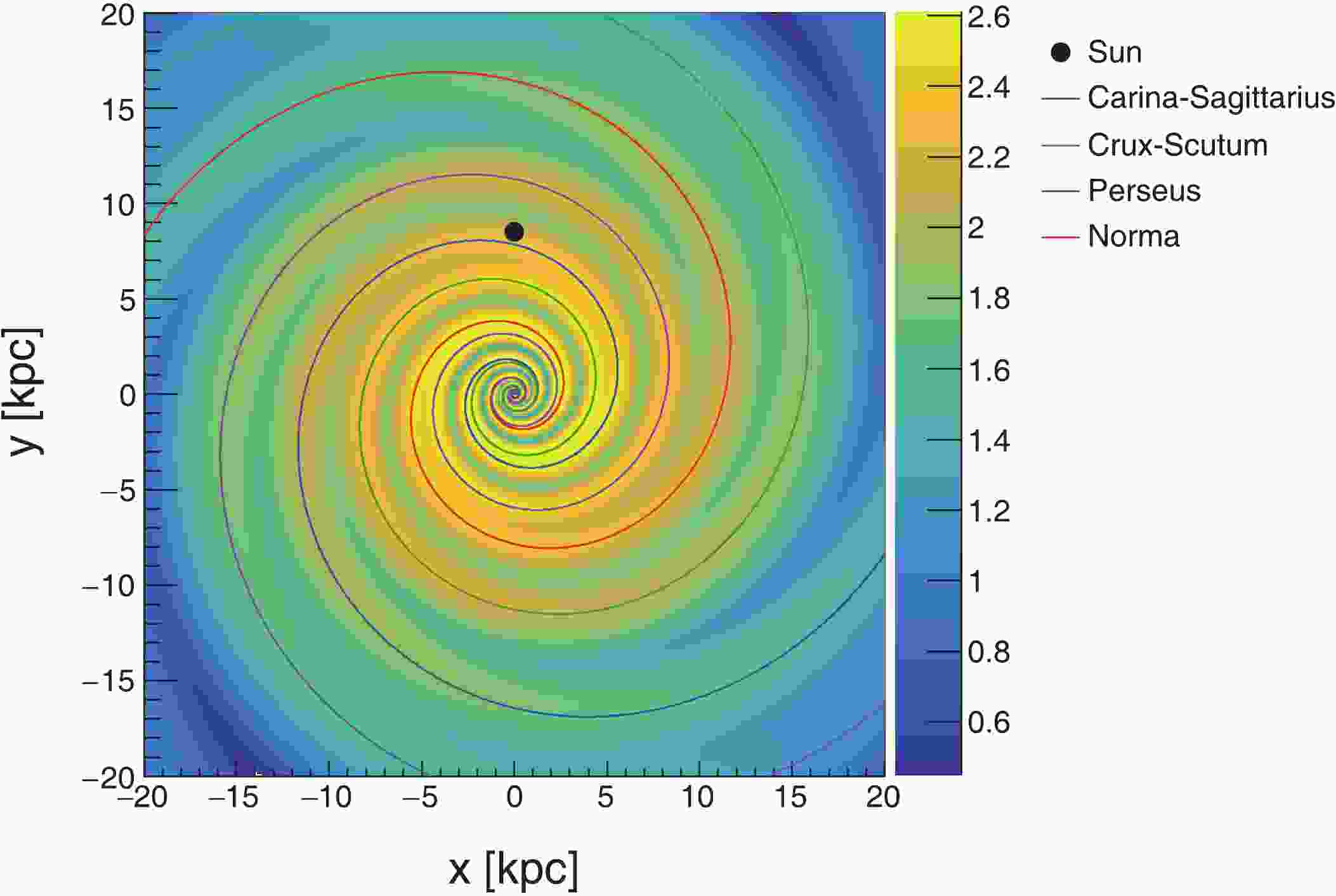
A large amount of observational evidence (see [59, 60] and references therein) has indicated that the Milky Way is a typical spiral galaxy. The high density gas concentrates in the spiral arms, which triggers a rapid star formation. The distribution of SNRs is highly correlated with the spiral arm pattern. In most past studies, the CR sources are typically approximated as axisymmetric-distributed sources, which is parameterized as

$ r_\odot $ represents the solar distance to the Galactic center, which is adopted as 8.5 kpc. The parameters $ \alpha $ and $ \beta $ are taken as 1.09 and 3.87, respectively in this work [61]. Perpendicular to the Galactic plane, the density of CR sources descends as an exponential function [61], with a mean value $ z_{s} = 100 $ pc. This approximation is plausible as the diffusion length of CRs is usually significantly longer than the characteristic spacing between the adjacent spiral arms. However, subject to the synchrotron radiation and inverse Compton scattering, the transport distance of the energetic electrons is significantly shorter, and the above approximation might become less accurate. Thus, the inclusion of a more realistic description of the spiral distribution is expected to have striking impact on the observed spectrum of high energy electrons. Observationally, there are still some uncertainties on the structure of the spiral arms, owing to our position in the Galaxy. The outer part of the Milky Way seems to have four arms, but the number of arms in the inner part is still being debated. The observations for the spiral structure and number of spiral arms are reviewed in [62, 63].

In this work, a model established by Ref. [64] is used to describe the spiral distribution of SNRs. The Galaxy consists of four major arms spiraling outward from the Galactic center. The locus of the i-th arm centroid expresses analytically as a logarithmic curve: $ \theta(r) = k^{i} \ln(r/r^{i}_{0}) + \theta_{0}^i $, where r is the distance to the Galactic center. The values of $ k^{i} $, $ r^{i}_{0} $, and $ \theta_{0}^i $ for each arm are listed in Table 1. Along each spiral arm, there is a spread in the normal direction, which follows a Gaussian distribution, i.e.,

i-arm	name	$k^{i}$/rad	$r^{i}_{0}$/kpc	$\theta_{0}^i$/rad
1	norma	4.25	3.48	0
2	carina-sagittarius	4.25	3.48	4.71
3	perseus	4.89	4.90	4.09
4	crux-scutum	4.89	4.90	0.95

Table 1.  Parameters $k^{i}$, $r^{i}_{0}$, and $\theta^{i}_{0}$ for four Galactic arm centroids.

where $ r_i $ is the inverse function of the i-th spiral arm's locus, and the standard deviation $ \sigma_i $ is taken to be $ 0.07 r_i $. The number density of SNRs at different radii remains consistent with the radial distribution in the axisymmetric case, i.e., Eq. (13). Fig. 1 shows the spatial distribution of SNRs in the spiral model. The solar system lies between the Carina-Sagittarius and Perseus spiral centroids.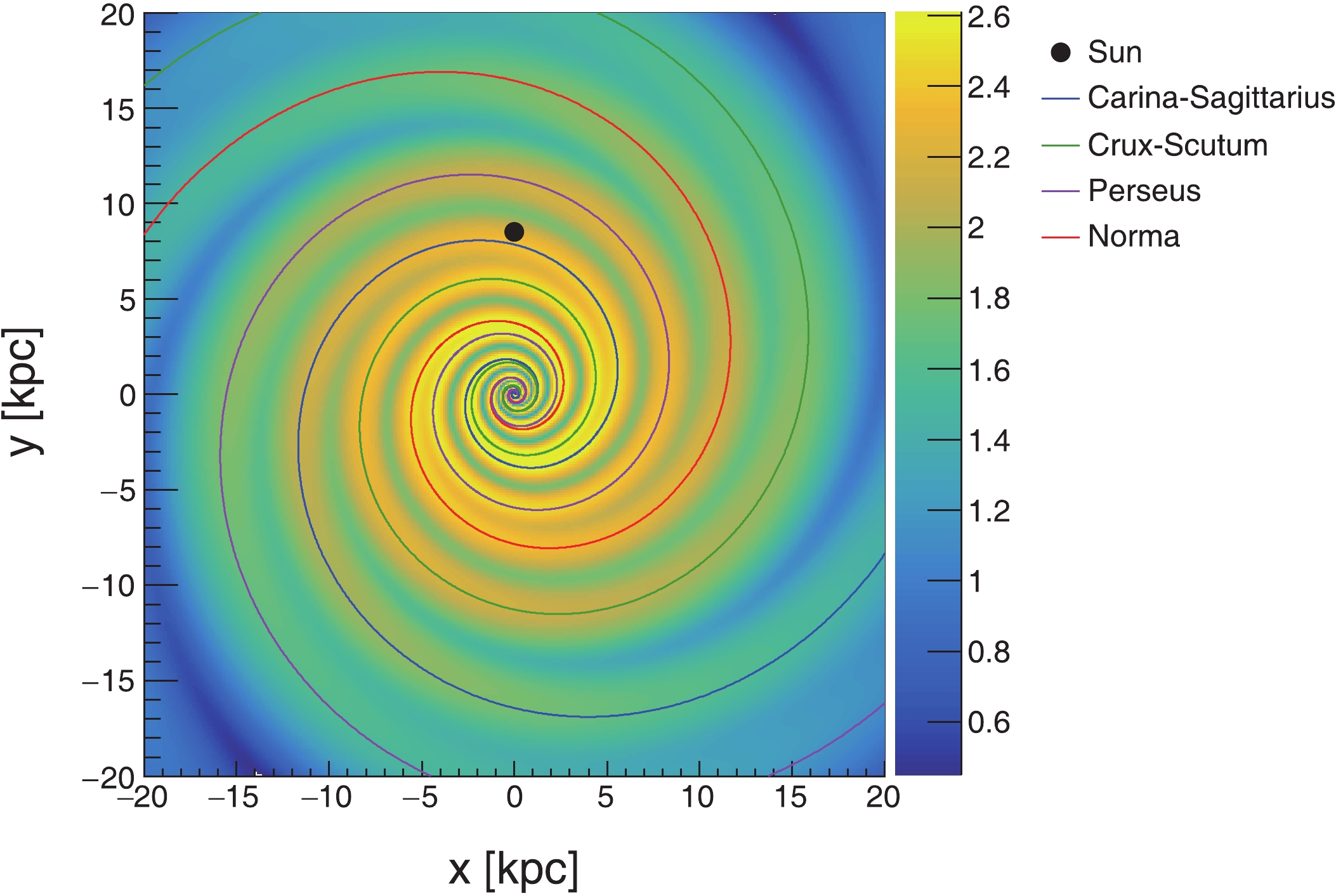

Figure 1.  (color online) Top view of density distribution of SNRs in the Galaxy. The Galaxy is assumed to have four spiral arms, with the Sun (depicted as a black point) lying bewteen the Garina-Sagittarius and Perseus arms, about 8.5 kpc away from the Galactic center.

Due to the energy loss during the propagation, the characteristic lifetime of energetic electrons and positrons at energy E is less than $ 2.3 \times 10^{5} (E/\rm TeV)^{-1} $ yr, which suggests that the corresponding diffusion distance is $ \sim 1 \cdot (E/\rm TeV)^{-1/3} $ kpc [65]. Therefore, at about TeV energies, the CR electrons and positrons originate from sources within 1 kpc around the solar system. Within 1 kpc, the number of generated SNRs is $ \sim 2.5 $ less than $ 10^5 $ yrs, assuming one supernova explosion per century. The continuity hypothesis is no longer valid. Studies show that the discrete effect of nearby CR sources could induce large statistical fluctuations [66, 67], especially at high energies. The role of nearby sources on the electrons and positrons has been studied in recent work (see [15, 31, 68] and references therein). In this work, we assume a nearby pulsar to account for the excess of positrons above $ \sim 20 $ GeV. The diffusion process of electrons/positrons injected instantaneously from a point source is described by a time-dependent propagation equation,

The corresponding Green's function $ G({{r}}-{{r}}^{\prime}, t- t^{\prime}, E) $ can be found in [69]. The energy dependence is taken as a single power-law distribution, namely

in which $ {\cal R}^{\rm e_{\pm}}_{\rm c} $ is the cutoff rigidity. For the local pulsar, a continuous injection process of electron-positron pairs is considered. The injection rate is time-dependent, which decays as pulsar-type [65], i.e.,

where $ t_i $ is the initial time of releasing electron-positron pairs. The characteristic duration $ \tau_0 $ is taken as $ 10^4 $ years as typically done in past literature, even if the value is uncertain and might vary for each specific pulsar, see e.g., [70]. The propagated spectrum is a convolution of the Green function and time-dependent injection rate $ Q_0(t) $ [65, 71], i.e.,

To demonstrate the effects of SDP and spiral distribution of background sources, the exploration of different propagation models is categorized as SDP with axisymmetric distribution (denoted as SDP + axis), SDP with spiral distribution (denoted as SDP + spiral) and homogeneous diffusion with axisymmetric distribution respectively. Notably, the situation of homogeneous diffusion considers two kinds of injection spectra for nuclei: one is the single power-law (denoted as HD + axis) and another has a spectral break above ~ 200 GV (denoted as HDB + axis). Under homogeneous diffusion, the free parameters that are fixed to accommodate the data are $ D_{0} $, $ \delta_{0} $, $ z_{h} $, and $ v_{\rm A} $. As for the SDP, two additional parameters are included, namely $ N_{\rm m} $ and $ \xi $ . The injection parameters of the background protons (heliums, electrons) are $ A^{{\rm p}/e^-} $, a, $ \nu^{{\rm p/He}/e^-}_1 $, $ \nu^{{\rm p/He}/e^-}_2 $, $ \nu^{{\rm p/He}/e^-}_3 $, $ {\cal R}^{{\rm p/He}/e^-}_{\rm br} $, $ {\cal R}^{\rm p/He}_{\rm brh} $, and $ {\cal R}_{\rm c} $. Here, $ A^{{\rm p}/e^-} $ is the normalization flux for the background protons (electrons). The parameter a represents the elemental abundance of primary helium compared with proton. The secondary electron and positron fluxes are rescaled by factor $ c^{e^+} $. The injection parameters of the local pulsar are $ q_{0} $, $ \gamma $, and $ {\cal R}_{\rm c}^{e_\pm} $. In addition, for proton, helium, electron, and positron, each has an individual modulation potential $ \phi $.

In this section, first of all, the transport parameters of four models are fixed by fitting the B/C ratio and proton spectrum. Then, the energy spectra of electrons and positrons obtained by four models are compared by fixed transport parameters. Finally, the anisotropies of all-electrons are calculated.

The benchmark values of the transport parameters for the four propagation models are fixed to explain the B/C ratio, as illustrated in Fig. 2. The orange, green, blue, and black solid lines represent HD + axis, HDB + axis, SDP + axis, and SDP + spiral, respectively. The corresponding transport parameters are listed in Table 2. Compared with the HD picture, both SDP scenarios favor a larger $ \delta_0 $ and halo size $ z_h $. This could also be inferred from the Bayesian analysis of the two-halo model [27]. In contrast to the HD model, the required alfvénic velocity is smaller, namely $ \sim 6 $ km/s. This can be understood as follows. In the SDP picture, both $ \delta $ and $ D_0 $ vary spatially and are smaller nearby the Galactic disk. A smaller $ D_{xx} $ corresponds to a larger $ D_{pp} $ according to Eq. (6). Hence, even if the alfvénic velocity is smaller, the diffusion-reacceleration still have a significant effect in the SDP model, compared with that in the HD model.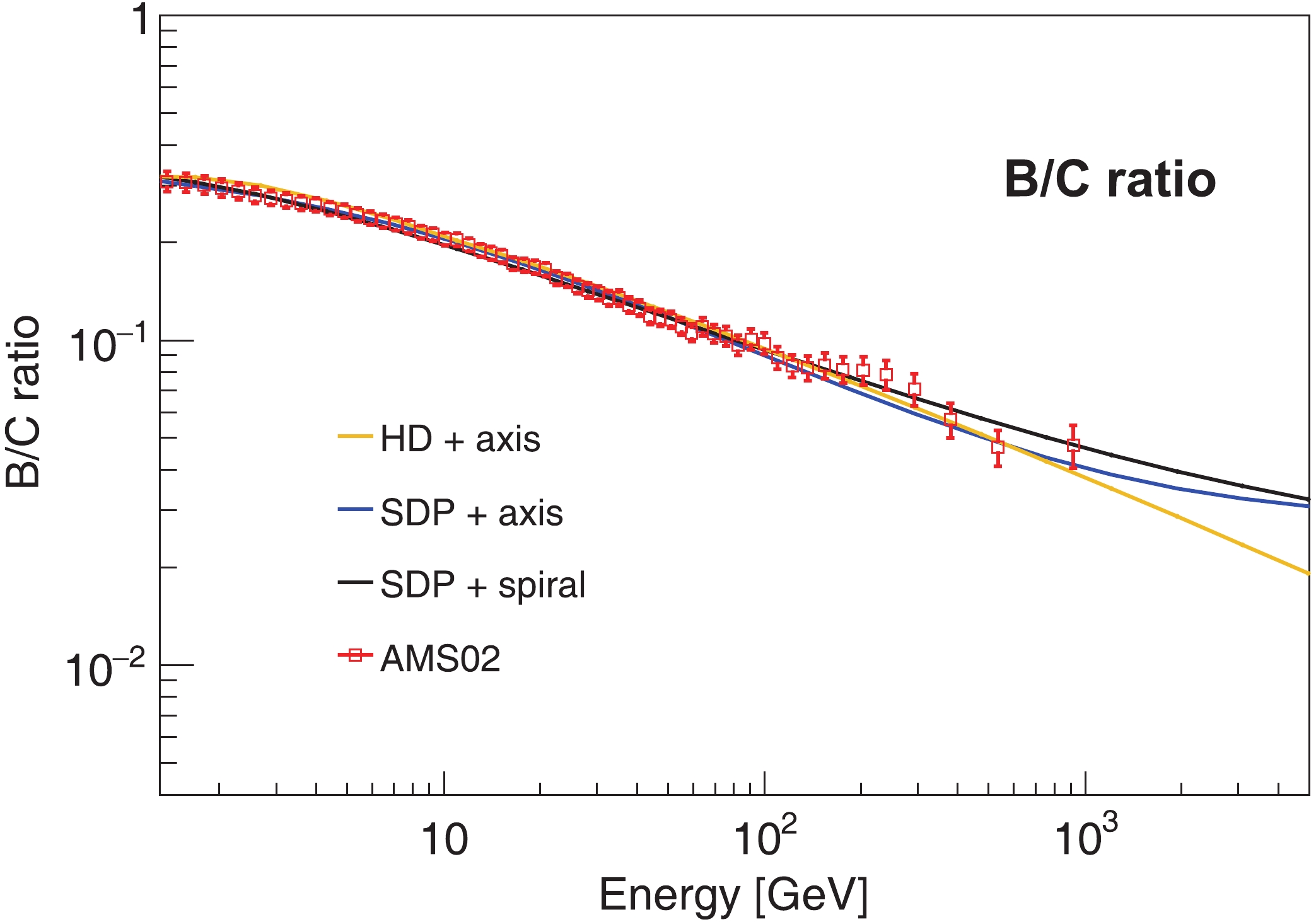

Figure 2.  (color online) Fit of the B/C ratio obtained by three propagation models, HD + axis (orange), SDP + axis (blue), and SDP + spiral (black). The data are taken from the AMS-02 experiment [72]. In this work, the benchmark values of the transport parameters for these propagation models are fixed by fitting the B/C ratio and proton spectrum.

Parameters	HD + axis	HDB + axis	SDP + axis	SDP + spiral
$D_{0}$/($10^{28}$cm2/s)	4.3	4.3	4.6	9.65
$\delta_{0}$	0.45	0.45	0.6	0.65
$z_{h}$/kpc	5	5	5	5
$N_{\rm m}$			0.141	0.24
$\xi$			0.1	0.12
$v_{\rm A}$/(km·s−1)	30	30	6	6
$A^{\rm p}\; /(\rm m^{-2}sr^{-1}s^{-1} GeV^{-1})^\dagger$	0.045	0.0435	0.0436	0.0436
$\nu_{1}^{\rm p}$	1.8	2.03	2.0	2.0
${\cal R}_{\rm br}^{\rm p}$/GV	9.9	11.0	5.5	5.5
$\nu^{\rm p}_{2}$	2.35	2.35	2.40	2.3
${\cal R}_{\rm brh}^{\rm p}$/GV		750
$\nu^{\rm p}_{3}$		2.11
$\phi^{\rm p}$/MV	500	800	800	800
${\cal R}_{\rm c}$/TV		145	86	82
a	0.0815	0.079	0.0568	0.0580
$\nu_{1}^{\rm He}$	1.8	2.03	2.0	2.0
${\cal R}_{\rm br}^{\rm He}$/GV	9.9	11.0	5.5	5.5
$\nu^{\rm He}_{2}$	2.35	2.43	2.51	2.41
${\cal R}_{\rm brh}^{\rm He}$/GV		370
$\nu^{\rm He}_{3}$		2.19
$\phi^{\rm He}$/MV	250	250	500	650
† The normalization is set at kinetic energy per nucleon $E_{\rm n} = 100$ GeV.

Table 2.  Parameters of the injection spectrum of the proton, helium, and propagation for HD + axis, HDB + axis, SDP + axis, and SDP + spiral models. For the HD and HDB models, the free propagation parameters are $D_{0}$, $\delta_{0}$ and $z_{h}$. For the SDP model, two additional parameters, namely $N_{m}$ and $\xi$, are included. The parameters of the injection spectrum of proton are the normalization $A^{\rm p}$, spectral indexes $\nu^{\rm p}_{1}$ below $R_{\rm br}^{\rm p}$, $\nu_{2}^{\rm p}$ between $R_{\rm br}^{\rm p}$ and $R_{\rm brh}^{\rm p}$, $\nu^{\rm p}_{3}$ above $R_{\rm brh}^{\rm p}$ and cutoff-rigidity $R_{\rm c}$. Further, the parameters of the injection spectrum of helium contain $\nu^{\rm He}_{1}$, $\nu^{\rm He}_{2}$, $\nu^{\rm He}_{3}$, $R_{\rm br}^{\rm He}$, and $R_{\rm brh}^{\rm He}$. The parameter a represents the elemental abundance of helium relative to the proton. $\phi^{\rm p}$ and $\phi^{\rm He}$ represent the modulation potential for proton and helium.

Notably, the SDP scenarios predict a flattening of the B/C ratio above 1 TeV. Compared with primaries, the hardening of secondaries principally has two sources: the hardening of the propagated primary spectrum and spatial-dependent propagation. Therefore, the propagated secondary spectrum is harder than the primary spectrum, which was substantiated by AMS-02 observations of secondary nuclei [73]. Therefore, an excess in the secondary-to-primary ratios is naturally generated under the SDP model [24, 27, 29]. Future precise measurements of the B/C ratio above TeV could verify this observation.

Figure 3 shows the propagated proton spectra obtained by four different propagation models. The red squares, gray inverted triangles, black crosses, and violet circles represent AMS-02, CREAM, DAMPE, and CALET measurements, respectively. The parameters of the proton injection spectrum are listed in Table 2. The HD model predicts that the propagated spectrum drops as a featureless power-law starting from tens of GeV (depicted by the orange line). This is visibly different from current observations. Compared with that in the HD model, the propagated proton spectrum under the HDB + axis assumption (shown as green line) is in good agreement with observations, where the spectral index changes $ \rm \nu^{p}_{2} = 2.35 $ to $ \rm \nu^{p}_{3} = 2.11 $ at rigidity $ \rm R_{brh}^{p} $ of 750 GV. In the SDP model, the high-energy CRs mainly originate from the neighboring regions around the solar system, and their transport mainly occurs in the IH region, where the rigidity dependence of the diffusion coefficient is weaker. Thus, the propagated proton spectrum exhibits significant hardening above $ \sim 200 $ GeV when $ \xi = 0.1 $, which efficiently reproduces the observations of AMS-02, CREAM, and CALET. Though DAMPE has released a similar hardening structure, its data is slightly different from the others. Therefore, our results do not fit well with DAMPE. Moreover, the distribution of CR sources makes no difference to the proton flux less than hundreds of GeV. Because the diffusion length of low energy protons is significantly longer than the characteristic interval of neighbouring spiral arms, the distribution of CR sources does not prominently modify the spectrum. However, for high-energy protons, the major diffusion region is at the IH region, whose thickness is comparable to the characteristic interval of neighbouring spiral arms. In this case, the source distribution could not be neglected. Above a few TeV, the spiral distribution enhances the proton flux, in comparison with the axisymmetric case.

Figure 3.  (color online) Corresponding propagated proton and helium spectra. The experimental data are taken from AMS-02 [72, 74] (red square), CREAM [75] (grey inverted triangle), DAMPE [76] (black cross), and CALET [77] (violet solid circles).

In addition, the predicted helium spectra are shown at the bottom of Fig. 3 as well. Table 2 displays the parameters of the injection spectrum of helium by four theoretical models. Observationally, the fitted injection spectrum of helium is 0.08 harder than proton in HDB, while it is 0.11 in the framework of SDP models. This may originate from the acceleration process at source region. To reproduce the flattening of proton and helium spectra above ~ 200 GeV, in the HDB model the spectral break of injection for proton and helium is tuned at rigidity $ \rm R_{brh}^{p} $= 750 GV and $ \rm R_{brh}^{He} $ = 370 GV, respectively. The cut-off rigidity $ {\cal R}_{\rm c} $ in HDB and SDP models is adjusted to 145 TV and around 85 TV.

It is worth to further evaluate the total energy of CRs injected by a single SNR in the SDP model, according to the normalization $ A^{\rm p} $. By approximating the SDP model as an one-dimensional two-halo model [24], the total energy of CRs above 1 GeV released by each SNR is roughly $ 4.5\times 10^{49} $ erg, assuming one supernova explosion per century. This is compatible with the transferred shock kinetic energy of the typical core-collaspe supernova.

Figure 4 demonstrates the calculated positron spectra obtained by different propagation models: HD + axis (upper left), HDB + axis (upper right), SDP + axis (lower left) and SDP + spiral (lower right). The blue and green lines are the components contributed by the background and local sources, respectively, where the background positron fluxes before and after rescaling are shown as blue dashed and solid lines, respectively. The black line is the sum of rescaled background and local fluxes. Table 3 lists the distance and age of local sources as well as the parameters for the injection spectrum of background and local sources.

Parameters	HD + axis	HDB + axis	SDP + axis	SDP + spiral
$A^{e^-}/(\rm m^{-2}sr^{-1}s^{-1} GeV^{-1})^\dagger $	0.16	0.16	0.30	0.30
$\nu_{1}^{e^-}$	1.7	1.69	1.53	1.14
$\nu^{e^-}_{2}$	2.8	2.81	2.9	2.72
${\cal R}_{\rm br}^{e^-}$/GV	4	4	5.1	5.1
$c^{e^+}$	2.0	1.8	1.4	1.0
r/kpc	0.35	0.25	0.2	0.25
t/yr	$3.0 \times 10^{5}$	$2.4 \times 10^{5}$	$2.2 \times 10^{5}$	$2.9 \times 10^{5}$
$q_{0}/{\rm{GeV}}^{-1}$	$3.56 \times 10^{50}$	$3.0 \times 10^{50}$	$ 1.29 \times 10^{50}$	$2.25 \times 10^{50}$
$\gamma$	1.94	2.012	2.46	2.40
${\cal R}^{e^{\pm}}_{\rm c}$/TV	8	8	8	8
$\phi^{e^{+}}$/MV	1400	1420	650	580
$\phi^{e^{-}}$/MV	1210	1210	660	620
† The normalization is set at kinetic energy $E = 10$ GeV.

Table 3.  Parameters of injection spectra of background electrons and local electron-positron pairs under HD + axis, HDB + axis, SDP + axis, and SDP + spiral models. The parameters of background electrons contain normalization factor $A^{e^{-}}$, spectral index $\nu^{e^{-}}_{1}$($\nu^{e^{-}}_{2}$) below (above) $R^{e^{-}}_{\rm br}$. $c^{e^{+}}$ represents the scale factor of the background positron flux. The corresponding parameters of local electron-positron pairs are the injection rate of electron-positron pairs $q_{0}$, spectral index $\gamma$, and cut-off rigidity $R^{e^{\pm}}_{\rm c}$. $\phi^{e^{+}}$ and $\phi^{e^{-}}$ are the modulation potentials for electrons and positrons, respectively.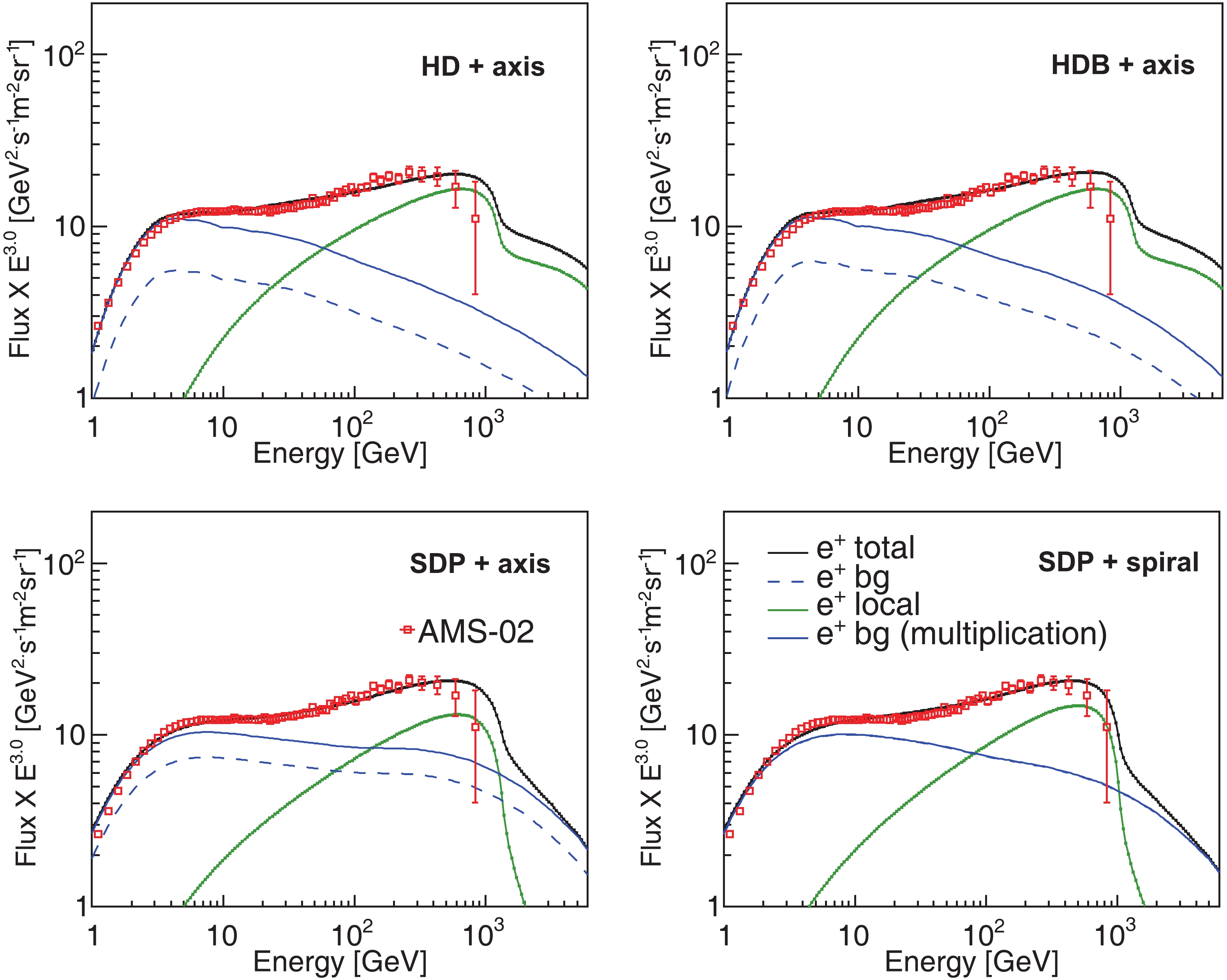

Figure 4.  (color online) Positron spectra computed by four propagation models, i.e., HD + axis (upper left), HDB + axis (upper right), SDP + axis (lower left), SDP + spiral (lower right). To consider the uncertainties from p-p collision cross-sections, propagation, etc., the secondary positrons obtaineed by HD + axis, HDB + axis, and SDP + axis models are multiplied by a scale factor $ c^{e^{+}} $. The red squares depict the measurements from the AMS-02 experiment [3]. The blue dashed and solid lines depict the background flux and the rescaled one (multiplied by $ c^{e^{+}} $) respectively, while the green solid lines represent the fluxes from the local source. The black solid line represents the sum of rescaled background and local fluxes. To describe the drop of positron above several hundreds of GeV recently unveiled by AMS-02, the cutoff rigidity of the local source $ {\cal R}^{ e_{\pm}}_{\rm c} $ is 8 TV.

In the HD model, the scale factor $ c^{e^+} $ reaches up to 2.0, and the studies of [56] and [15] come to a similar conclusion. Influenced by a noticeable growth of proton fluxes above tens of GeV, the HDB scenario would undoubtedly contribute more background components of positrons than that of HD model. Thus, its corresponding scale factor naturally decreases down to 1.8. However, the SDP model brings about a broken power-law in the propagated positron spectrum, such that above tens of GeV, the positron spectrum becomes flatter. This appreciably enhances the secondary positron flux at higher energy. Compared with nuclei, the broken energy shifts from $ \sim 200 $ GeV to $ \sim 20 $ GeV, due to the energy loss of positrons during the transport. As observe, $ c^{e^+} $ in the SDP with axisymmetric distribution drops dramatically to 1.4. According to [54], [55], and [27], the uncertainties in production cross-section models differ from the secondary positron flux up to tens of percentages. The uncertainties from the propagation and injection are ~30% at ~100 GeV, and gradually increase with energy [27]. In the model of spiral distribution, $ c^{e^+} $ further reduces to 1.0 for the propagated parameters in Table 3.

In all four models, the injection spectrum of the local source is harder than that of background. However, in the HD and HDB models, the difference between both is larger. The power index of local source is around 2.00, while it is 2.8 for the background SNRs. However, in the SDP models, the obtained power index of local pulsar increases and their difference becomes smaller. Moreover, it is noteworthy that in the HD models, the propagated positron spectrum shows a pronounced high-energy tail, which is obviously different from the high-energy sharp fall-off under the assumption of a transient injection [15]. This is due to the continuous injection process of pulsar [65, 78]. Likewise, a similar phenomenon is also visible in the corresponding electron spectra, as shown in Fig. 5. However, this feature disappears in the SDP models. Instead, the energy spectra above TeV energies slowly decline. As the diffusion process is significantly slower in the vicinity of the Galactic disk, the energetic electrons from the local source suffer more energy loss such that most of them were exhausted before arriving at the solar system. To fit the high-energy drop, the cutoff rigidity of the local injection electron/positron spectrum is 8 TV.

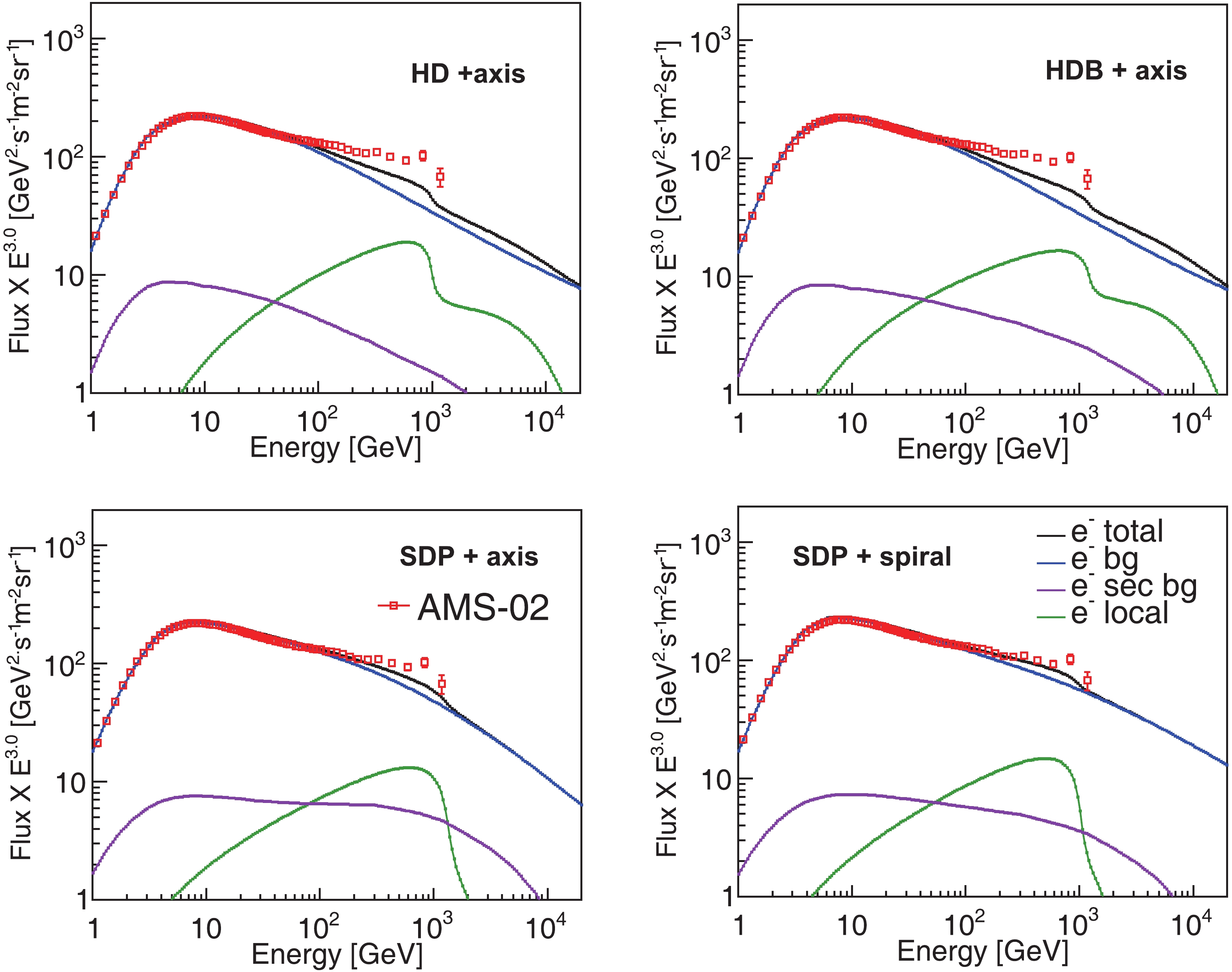
Figure 5.  (color online) Electron spectra computed by four transport models, HD + axis (upper left), HDB + axis (upper right), SDP + axis (lower left), and SDP + spiral (lower right). The red squares depict the measurements from the AMS-02 experiment [7]. The blue and violet lines represent the background primary and secondary electron fluxes, respectively, while the green line refers to the electron flux from the local source.

The observations confirm that there is a hardening above ~40 GeV in the electron spectrum, which indicates a primary component. Under the model of a local pulsar, the contribution of electrons from the local source is determined by the positron data. Above ~100 GeV, the electron data could not be described both in the HD model, even with a local source. This is due to the excess of primary electron flux. In the observed electron flux, this contains both primary and secondary components, despite the latter being far smaller than the former. In contrast, in either the propagation process or the local pulsar, almost the same amount of electrons and positrons are generated. Thereupon, the difference between electrons and positrons is expected to be within the primary components, and this is described by a single power-law spectrum in the conventional diffusion model. However, the analysis of [5] revealed that there is also a significant excess in this component. One of the origins for the extra electrons is the local SNRs. In a recent work by [15], to efficiently describe both electron and positron spectra, a nearby supernova remnant surrounding by a giant molecular cloud is introduced, where the additional electron-positron pairs, apart from the primary electrons, are produced inside the SNR through interactions between CRs and the molecular clouds. For the HDB model, its flux of propagated secondary electrons is enhanced slightly, which is attributed to the hardening of the proton spectrum. In comparison with the primary component, this contribution of secondary electrons is small. Likewise, it is evident that above ~ 100 GeV, the electron spectrum of the HDB model could not reproduce the AMS-02 observations. In the SDP model, the calculated electron flux is flatter, such that the background electrons significantly augment at high energy, as shown in Fig. 5. The overabundant primary electrons are attributed to the effect of SDP. Hence, the observed electron spectrum could be better described by the SDP model. Further, the modulation potential $ \phi $ in the conventional DR model is larger [56], that is, 1200 MeV for electron and 1400 MeV for positron, respectively. However, in the SDP model, its value is greatly reduced, which is approximately ~650 MeV.

The electron and positron spectra are added for further comparison with the observed all-electron spectrum, which is shown in Fig. 6. The experimental data of AMS-02, CALET, DAMPE, and H.E.S.S are represented by red squares, violet circles, black crosses, and green inverted triangles, respectively. From ~50 GeV to ~1 TeV, the DAMPE experiment apparently disagrees with AMS-02 and CALET. Furthermore, the H.E.S.S experiment extended its measurement of the all-electron spectrum up to 20 TeV, and the data is in a good agreement with both AMS-02 and CALET at around TeV energies. Therefore, we do not fit the DAMPE data in this work. We compare the calculated all-electron spectra of the four models with the observations of AMS-02, CALET, and H.E.S.S experiments. The all-electron spectra is well reproduced by the SDP + spiral distribution scenario within the entire energy range. The break around TeV is due to the local source, while the power-law drop above that energy arises from the background components.

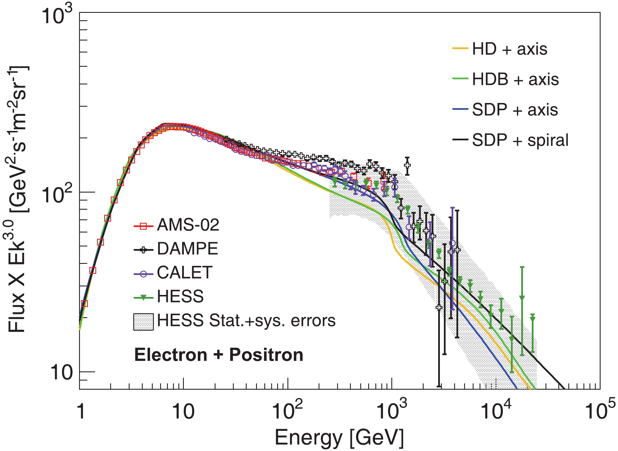
Figure 6.  (color online) All-electron (electron + positron) spectra calculated by four models. The red squares, violet circles and green inverted triangles depict the data of AMS-02 [7], CALET [79], and HESS [9], respectively. The black crosses correspond to the measurements of the DAMPE experiment [6].

The electrons and positrons above TeV mainly originate from the local sources within 1 kpc around the solar system. Similar to CR nuclei [80, 81], the local source may also leave an imprint on the all-electron anisotropy as well as the energy spectra. The dipole anisotropy is defined as

The anisotropies of the electron + positron from the local sources have been studied in the recent work based on the homogeneous diffusion model (see [15, 68, 78] and references therein). In this work, both background sources and the local pulsar could contribute to the anisotropy. Because the Galactic SNRs concentrate at the inner disk, there is a radial CR streaming coming from the Galactic center. Meanwhile, under spiral distribution, the SNRs are distributed along the spiral arms, and there is another CR streaming perpendicular to the direction of the Galactic center. Thereupon, the background anisotropy is a combined effect of two directions.

Figure 7 illustrates the energy dependence of the anisotropy of the electron + positron when the local pulsar is along the direction of the Galactic center. The blue solid lines denote the anisotropy from the background, and the green lines show the anisotropy generated by the local pulsar when neglecting the background anisotropy. The black lines depict sum of the background and local anisotropies. In the HD and HDB models, the local source dominates the anisotropy, and the total anisotropy is very large, which is close to the observational upper limits. This is caused by the larger diffusion coefficient nearby the solar system. However, in the SDP models around the Galactic disk, the diffusion coefficient is significantly smaller. Therefore, contrary to the HD and HDB models, the SDP models predict a very small background anisotropy. Even when taking the local source into account, the total anisotropy is still well below the current upper limits, compared with the conventional propagation models [78].

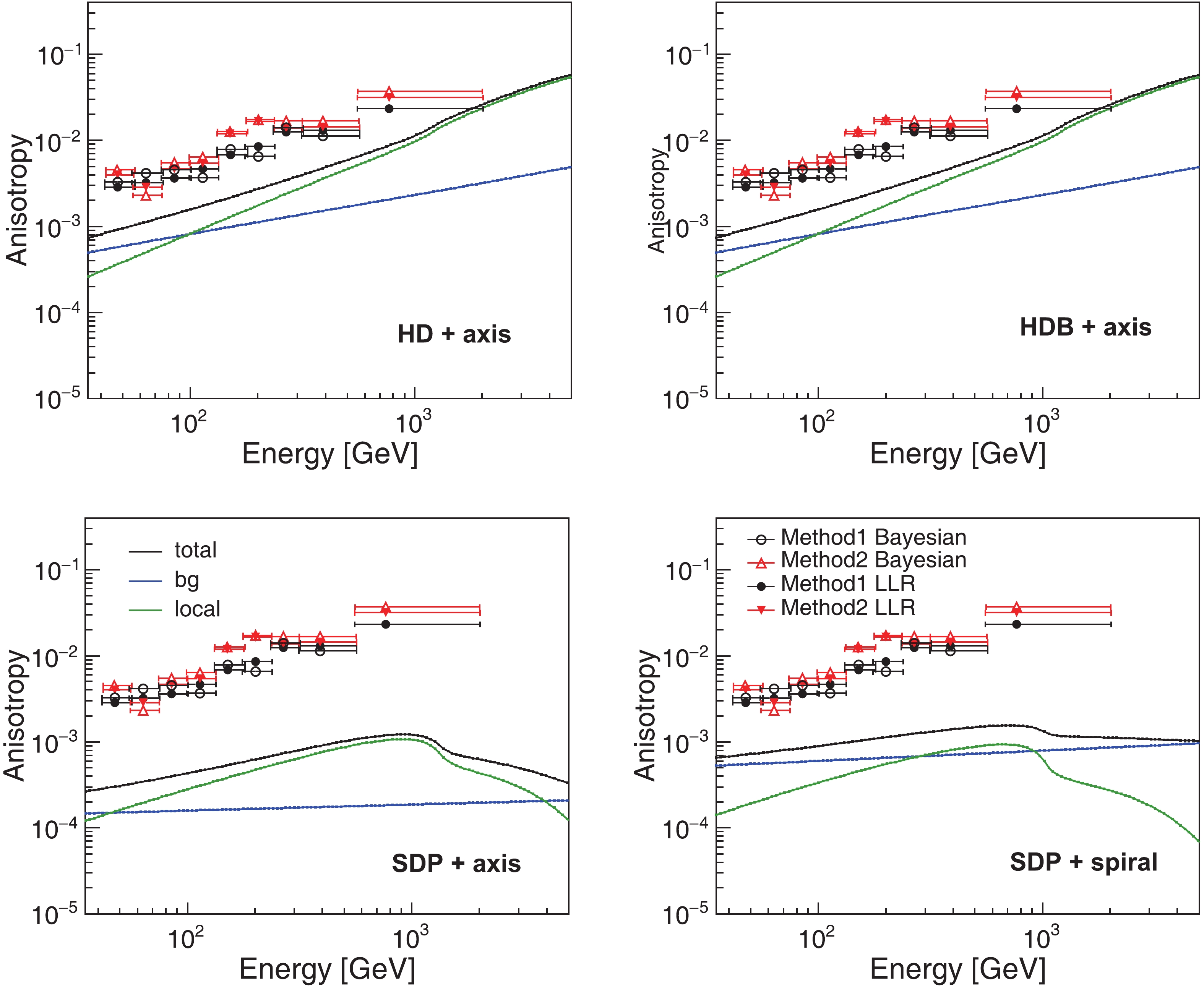
Figure 7.  (color online) Anisotropies of the electron with the local source along the direction of Galactic center obtained by the models HD + axis (upper left), HDB + axis (upper right), SDP + axis (lower left), and SDP + spiral (lower right). The blue, green, and black solid lines represent the anisotropies of background, local source, and their sum, respectively. Both black and red markers are the upper limits set by the Fermi-LAT experiment [82].

Fig. 8 illustrates the same electron anisotropies, but with the local pulsar in the direction of anti-Galactic center. The CR streaming from the local pulsar opposes that of the background, which could further lower the total anisotropy. When the CR streaming from local pulsar is comparable to that of background, the total anisotropy reaches a minimum. In the HD and HDB models, from tens of GeV to ~1 TeV, the local source consistently dominates, except for the lower energy, where the background streaming takes effect. A similar case occurs in the SDP + axis distribution. However, for the SDP + spiral distribution model, the background and local streaming are comparable at ~100 GeV and ~2 TeV, respectively, and there are two minimums in the total anisotropy. Within this energy range, the anisotropy is dominated by the local pulsar, while background sources play a major part at the remaining energies.

Figure 8.  (color online) Anisotropies of the electron with the local source in the direction of anit-Galactic center.

With the improvements in the energy resolution, particle identification and available observation range of both space-based and ground-based experimental instruments, the measurements of CR electrons and positrons have become increasingly precise in the recent years. The current measurements unveil more unexpected features and raise new challenges to the conventional propagation model. In this work, we study the effects of SDP and spiral distribution by explaining the latest electron and positron observations. To demonstrate both effects, four kinds of propagation models are compared. In comparison with the homogeneous diffusion model, SDP could prominently enhance the background electron and positron flux at high energy, such that the excess of the primary electron could be accounted for by the SDP effect without introducing other local SNRs. Both electron and positron spectra could be explained by the SDP model. In the meantime, the all-electron spectrum up to 25 TeV could also be naturally described in the SDP + spiral distribution scenario. The break around TeV is generated by the local source, and the high-energy power-law drop is principally attributed to the background components.

In the local source model, both the distance and age are evaluated by fitting the AMS-02 observations. The local pulsar, e.g., with $ t = 2.9\times10^{5} $ years and $ r = 0.25 $ kpc in the SDP + spiral model, is very close to the Geminga pulsar ($ t = 342 $ kyr and $ r = 0.25 $ kpc). We use some properties of Geminga listed in the ATNF catalog [83] to further investigate the converted efficiency to electron-positron pairs of the local pulsar. According to the parameters given in Table 3, the total rotational energy loss is estimated as $ 9.83\times10^{48} $ ergs. The total injection energy of electron-positron pairs from this pulsar is $ 1.97\times10^{48} $ ergs, and the corresponding converted efficiency is nearly 20%. These values are consistent with the general estimation. For the local pulsars assumed in the other models, the corresponding estimations are also compatible with the expected estimation of a mature pulsar.

The anisotropy of the electron is calculated by four models. In the conventional model, the total anisotropy is dominated by the local source, and it is very close to the upper limits set by the Fermi-LAT experiment due to the larger diffusion coefficient. However, in the SDP model, owing to the smaller diffusion coefficient around the Galactic disk, the level of the background anisotropy is significantly lower. In this case, even including a local source, the total anisotropy remains considerably small. The precise future measurements of electron anisotropy by the DAMPE, LHAASO [84], and HERD [85] experiments could test our model.

DRAGON [53] is available at https://github.com/cosmicrays