


 Abstract
 HTML
HTML Reference
 Related
 PDF
PDF


-
The heavy-to-light exclusive weak decays provide a fertile ground for testing the standard model (SM) and investigating the physics beyond it. In the calculation of the amplitudes of these decays, some nonperturbative quantities, such as the decay constant, distribution amplitudes, and form factors, are essential and important inputs. For example, the dominant contribution to the amplitude of
$ b\to s\gamma $ radiative decay is proportional to the form factors associated with the tensor current. These quantities can be evaluated by numerous different approaches, such as the Wirbel-Stech-Bauer model [1], lattice QCD [2], QCD sum rules [3, 4], and light-front quark models (LF QMs) [5–9].The LF QMs can be roughly classified into two types: the standard light-front (SLF) QM [5, 6] and the covariant light-front (CLF) QM [7–9]. The SLF QM is a relativistic quark model based on the LF formalism [10] and LF quantization of QCD [11] provides a conceptually simple and phenomenologically feasible framework for evaluating nonperturbative quantities. However, the matrix element evaluated in this approach lacks a manifestation f the Lorentz covariance, and therefore, it is subsequently replaced by the CLF QM. A popular framework for the CLF QM was developed by Jaus [9] with the help of a manifestly covariant Bethe-Saltpeter (BS) approach as a guide to the calculation. In this approach, the zero-mode contributions can be efficiently determined, and the result of the matrix element is expected to be covariant because of the
$ \omega $ -dependent spurious contributions, where$ \omega^\mu = (0,2,{\bf 0}_\bot) $ is the light-like four-vector used to define the light-front by$ \omega\cdot x = 0 $ . The$ \omega $ -dependent contributions may violate the covariance, and they can be eliminated by inclusion of zero-mode contributions [9]. The LF QMs have been widely used to evaluate some nonperturbative quantities of hadrons, and they are further applied to phenomenological researches [12–78]. In this study, we focus on the form factors related to the tensor current matrix elements.The tensor form factors of
$ B\to \pi\,,K\,,\rho $ , and$ K^* $ transitions have been evaluated in the SLF QM with$ { \bf q}_\bot = 0 $ frame [79]. Within the CLF QM, the tensor form factors of$ B_{u,d}\to V\,,A $ , and T transitions are calculated in Ref. [80] and are corrected in Refs. [81, 82]; the corrected theoretical results are further applied to the phenomenological studies of some radiative B and$ B_s $ decays [82] and radiative D and$ D_s $ decays [83]. It is worth checking these previous results of tensor form factors and evaluating the transitions that were not hereto considered. Further, it should be noted that above-mentioned studies are performed within the traditional CLF QM [9], which exhibits covariance and self-consistence problems.The traditional CLF approach [9] has long been known to suffer from a self-consistence problem in the vector meson system. For example, the CLF results for the decay constant of the vector meson,
$ f_V $ , obtained via longitudinal ($ \lambda = 0 $ ) and transverse ($ \lambda = \pm $ ) polarization states, are inconsistent with each other, i.e.,$ [f_V]^{\lambda = 0}\neq [f_V]^{\lambda = \pm} $ [60], because the former receives an additional contribution characterized by the$ B_1^{(2)} $ function. Some analyses have been made in Ref. [84], and the authors present a possible solution to the self-consistence problem by introducing a modified correspondence between the covariant BS approach and the LF approach (named as type-II scheme [84]), which requires an additional$ M\to M_0 $ replacement relative to the traditional correspondence scheme (referred to as the Type-I scheme [84]).In our previous studies [85–87], the self-consistence problem has also been studied in detail via
$ f_{P,V,A} $ and form factors of$ P\to (P,V) $ and$ V\to V $ transitions, associated with the (axial-)vector current, and the modified Type-II correspondence scheme is tested in detail as a solution to the self-consistence problem [84]. Furthermore, we have also found that the covariance of the traditional CLF QM in fact cannot be maintained strictly due to the residual$ \omega $ -dependent contributions; the self-consistence and covariance problems have the same origin and can be resolved simultaneously by employing the modified Type-II scheme. In this study, we extend our previous efforts on above issues to the tensor form factors of$ P\to P,\,S,\,V $ , and A transitions, and update the theoretical results within a self-consistent scheme. We also show another “new” self-consistence problem of the CLF QM, which has not been noted before.Our paper is organized as follows. In Section 2, we briefly review the SLF and the CLF QMs for the convenience of discussion, and then present our theoretical results for the tensor form factors of
$ P\to P,\,S,\,V $ , and A transitions. In Section 3, the self-consistency and covariance of CLF QM are discussed in detail, and our numerical results for the tensor form factors of some$ c\to q,\,s $ and$ b\to q,\,s\,,c $ ($ q = u,d $ ) induced$ P\to P,\,S,\,V $ , and A transitions are presented. Finally, we provide a summary in Section 5. Previously obtained theoretical results are collected in Appendix A for convenience of discussion and comparison, and the values of input parameters used in the computation are collected in Appendix B. -
The hadronic matrix elements associated with tensor operators are commonly factorized in terms of tensor form factors as
$ \langle P''(p{''})|\bar q''_1 \sigma^{\mu\nu}q'_1|P'(p{'}) \rangle =i(P^{\mu}q^{\nu}-P^{\nu}q^{\mu})\dfrac{F_T(q^2)}{M'+M''}\,, $

(1) $ \langle S''(p'')|\bar q''_1 \sigma^{\mu\nu}\gamma_5q'_1|P'(p{'}) \rangle = i(P^{\mu}q^{\nu}-P^{\nu}q^{\mu})\dfrac{U_T(q^2)}{M'+M''}\,, $

(2) for
$ P\to P $ and$ P\to S $ transitions, respectively, where$ P = p'+p'' $ ,$ q = p'-p'' $ , and$ M^{\prime(\prime\prime)} $ is the mass of the initial (final) state. For the$ P\to V $ and$ P\to A $ transitions, the tensor form factors are defined as$ \begin{split} & \langle V(p'',\epsilon) | \bar{q}''_1 \sigma^{\mu\nu} \ q'_1 |P(p') \rangle \\ = &-\varepsilon^{\mu\nu\alpha\beta}\left\{ -\epsilon_{\alpha }^*P_\beta T_1(q^2)+\dfrac{M'^2-M''^2}{q^2}\epsilon_{\alpha }^*q_\beta\left[ T_1(q^2)- T_2(q^2)\right] \right.\\ &\left.-\dfrac{\epsilon^{ *}\cdot q}{q^2} P_\alpha q_\beta\left[T_1(q^2)- T_2(q^2)-\dfrac{q^2}{M'^2-M''^2} T_3(q^2) \right]\right\}\,,\\[-18pt] \end{split} $

(3) $ \begin{split} &\langle \,^{i}\!A(p'',\epsilon) | \bar{q}''_1 \sigma^{\mu\nu}\gamma_5 \ q'_1 |P(p') \rangle \\ = &\varepsilon^{\mu\nu\alpha\beta}\left\{ -\epsilon_{\alpha }^*P_\beta T_1^{(i)}(q^2)+\dfrac{M'^2-M''^2}{q^2}\epsilon_{\alpha }^*q_\beta\left[ T_1^{(i)}(q^2)- T_2^{(i)}(q^2)\right]\right.\\ & \left. -\dfrac{\epsilon^{ *}\cdot q}{q^2} P_\alpha q_\beta\left[T_1^{(i)}(q^2)- T_2^{(i)}(q^2)-\dfrac{q^2}{M'^2-M''^2} T_3^{(i)}(q^2) \right]\right\}\,, \end{split} $

(4) where
$ \varepsilon^{0123} = 1 $ ;$ ^{i}\!A $ with$ i = 1 $ and$ 3 $ denote$ ^{2S+1}\!L_J $ $ = $ $ ^1\!P_1 $ and$ ^3\!P_1 $ states, respectively; and for the form factors in Eq. (4), the superscript “$ (i) $ ” with$ i = 1 $ and$ 3 $ are added to distinguish P$ \to $ $ ^{1}\!A $ and P$ \to $ $ ^{3}\!A $ transitions. The definitions, Eqs. (3) and (4), are equivalent to$ \langle V(p'',\epsilon) | \bar{q}''_1 \sigma^{\mu\nu} q_\nu \ q'_1 |P(p') \rangle = \varepsilon^{\mu\nu\alpha\beta}\epsilon_{\nu}^* P_\alpha q_\beta T_1(q^2)\,, $

(5) $ \begin{split} & \langle V(p'',\epsilon) | \bar{q}''_1 \sigma^{\mu\nu}\gamma_5 q_\nu \ q'_1 |P(p') \rangle \\ = &-i\left[ (M'^2-M''^2)\epsilon^{\mu *} -\epsilon^*\cdot q P^\mu \right]T_2(q^2)\\ &-i\epsilon^*\cdot q\left[ q^\mu-\dfrac{q^2}{M'^2-M''^2}P^\mu \right]T_3(q^2)\,, \end{split} $

(6) and
$ \langle \,^{i}\! A(p'',\epsilon) | \bar{q}''_1 \sigma^{\mu\nu}\gamma_5 q_\nu \ q'_1 |P(p') \rangle = -\varepsilon^{\mu\nu\alpha\beta}\epsilon_{\nu}^* P_\alpha q_\beta T_1^{(i)}(q^2)\,, $

(7) $ \begin{split} &\langle \,^{i}\!A(p'',\epsilon) | \bar{q}''_1 \sigma^{\mu\nu} q_\nu \ q'_1 |P(p') \rangle \\ = &i\left[ (M'^2-M''^2)\epsilon^{\mu *} -\epsilon^*\cdot q P^\mu \right]T_2^{(i)}(q^2)\\ &+i\epsilon^*\cdot q\left[ q^\mu-\dfrac{q^2}{M'^2-M''^2}P^\mu \right]T_3^{(i)}(q^2)\,, \end{split} $

(8) respectively.
The main function of LF approaches is to evaluate the current matrix element of the
$ M'\to M'' $ transition,$ {\cal B} \equiv \langle M''(p'') | \bar{q}''_1 (k_1'')\Gamma q'_1(k_1') |M'(p') \rangle \,,\quad \Gamma = \sigma_{\mu\nu},\,\sigma_{\mu\nu}\gamma_5,\,... $

(9) which will be further used to extract the form factors by matching to the definitions given above.
-
The SLF and CLF QMs were fully illustrated in e.g., Refs. [5, 6, 12, 13, 29] and Refs. [9, 59, 60, 84], respectively. One may refer to these literatures for detail. In this study, we assume the same notations and conventions as Refs. [85–87].
In the framework of the SLF QM, the matrix element, Eq. (9), can be written as [85–87]
$\begin{split} {\cal B}_{\rm {SLF}} = &\sum\limits_{h'_1,h''_1,h_2} \int \frac{{{\rm{d}}} x \,{{\rm{d}}}^2{ {\bf k}_\bot'}}{(2\pi)^3\,2x} {\psi''}^{*}(x,{\bf k}_{\bot}''){\psi'}(x,{\bf k}_{\bot}') S''^{\dagger}_{h''_1,h_2}(x,{\bf k}_{\bot}'')\,\\ & \times C_{h''_1,h'_1}(x,{\bf k}_{\bot}',{\bf k}_{\bot}'')\,S'_{h'_1,h_2}(x,{\bf k}_{\bot}')\,, \\[-16pt] \end{split}$

(10) where
$ C_{h''_1,h'_1}(x,{\bf k}_{\bot}',{\bf k}_{\bot}'') \equiv \bar{u}_{h''_1}(x,{\bf k}_{\bot}'') \Gamma u_{h'_1}(x,{\bf k}_{\bot}') $ corresponds to the operator in Eq. (9); x and$ { \bf k}_\bot' $ are the internal LF relative momentum variables. The momenta of quark$ q_1' $ and spectator anti-quark$ \bar{q}_{2} $ in the initial state have been written in terms of$ (x,{ \bf k}_\bot') $ as$ k_1'^+ = xp'^+\,,\;\;\, {\bf k}_{1\bot}' = x{\bf p}_{\bot}'+{\bf k}_{\bot}' \,;\quad k_2^+ = \bar{x}p'^+ \,,\;\;\, {\bf k}_{2\bot} = \bar{x}{\bf p}_{\bot}'-{\bf k}_{\bot}'\,,\\ $

(11) where
$ \bar{x} = 1-x $ . For the convenience of calculation, it is usually assumed that the initial state moves along the z-direction, which implies that$ {\bf p}_{\bot}' = 0 $ . Taking the convenient Drell-Yan-West frame,$ q^+ = 0 $ , where$ q\equiv p'-p'' = k_1'-k_1'' $ is the momentum transfer, the momentum of quark$ q_1'' $ in the final state can be written as$ k_1''^+ = xp''^+ = xp'^+\,,\quad\, {\bf k}_{1\bot}'' = x{\bf p}_{\bot}''+{ \bf k}_\bot'' = -x{ \bf q}_\bot+{ \bf k}_\bot''\,, $

(12) where
$ { \bf k}_\bot'' = { \bf k}_\bot'-\bar{x}{ \bf q}_\bot $ .In Eq. (10),
$ \psi(x,{ \bf k}_\bot) $ and$ S_{h_1,h_2}(x,{ \bf k}_\bot) $ are the radial and the spin-orbital wavefunctions (WFs). For the former, we adopt commonly used Gaussian-type WFs, which are written as$ \psi_s(x,{ \bf k}_\bot) = 4\dfrac{\pi^{\frac{3}{4}}}{\beta^{\frac{3}{2}}} \sqrt{ \dfrac{\partial k_z}{\partial x}}\exp\left[ -\dfrac{k_z^2+{ \bf k}_\bot^2}{2\beta^2}\right]\,, $

(13) $ \psi_{p}(x,{ \bf k}_\bot) = \dfrac{\sqrt{2}}{\beta}\psi_s(x,{ \bf k}_\bot) \,, $

(14) for s-wave and p-wave mesons, respectively. The Gaussian parameters
$ \beta $ can be determined by fits to data;$ k_z $ is the relative momentum in the z-direction and can be written as$ k_z = \left(x-\dfrac{1}{2}\right)M_0+\dfrac{m_2^2-m_1^2}{2 M_0}\,, $

(15) with the invariant mass defined by
$ M_0^2 = \dfrac{m_1^2+{\bf k}_{\bot}^2}{x}+\dfrac{m_2^2+{\bf k}_{\bot}^2}{\bar{x}}\,. $

(16) For the latter,
$ S_{h_1,h_2}(x,{\bf k}_{\bot}) $ can be obtained by the interaction-independent Melosh transformation, and finally written as a covariant form [13, 60],$ S_{h_1,h_2} = \dfrac{\bar{u}(k_1,h_1)\Gamma_M v(k_2,h_2)}{\sqrt{2} \hat{M}_0}\,, $

(17) where
$ \hat{M}_0^2 = M_0^2-(m_1-m_2)^2 $ . For the P, S, V, and A states,$ \Gamma_M $ has the form$\Gamma_P =\gamma_5\,, $

(18) $ \Gamma_V = -\not\!\hat{\epsilon}+\dfrac{\hat{\epsilon}\cdot (k_1-k_2)}{D_{V,{\rm {LF}}}}\,, $

(19) $ \Gamma_S = \dfrac{\hat{M}_0^2}{2\sqrt{3}M_0}\,, $

(20) $ \Gamma_{ ^1\!A} = -\dfrac{1}{D_{1,{\rm {LF}}}}\hat{\epsilon}\cdot (k_1-k_2) \gamma_5\,, $

(21) $ \Gamma_{ ^3\!A} = -\dfrac{\hat{M}_0^2}{2\sqrt{2} M_0}\left[ \not\!\hat{\epsilon}+\dfrac{\hat{\epsilon}\cdot (k_1-k_2)}{D_{3,{\rm {LF}}}} \right]\gamma_5 \,, $

(22) where
$ D_{V,{\rm {LF}}} = M_0+m_1+m_2 $ ,$ D_{1,{\rm {LF}}} = 2 $ ,$ D_{3,{\rm {LF}}} = \hat{M}_0^2/ (m_1-m_2) $ and$ \hat{\epsilon}^{\mu}_{\lambda = 0} = \dfrac{1}{M_0}\left(p^+,\dfrac{-M_0^2+{\bf p}_{\bot}^2}{p^+},{\bf p}_{\bot}\right)\,, $

(23) $ \hat{\epsilon}^{\mu}_{\lambda = \pm} = \left(0,\dfrac{2}{p^+}{ \epsilon}_{\bot}\cdot {\bf p}_{\bot}, { \epsilon}_{\bot}\right)\,, \quad { \epsilon}_{\bot}\equiv \mp \dfrac{(1,\pm i)}{\sqrt{2}}\,. $

(24) Using the formulas given above, the explicit expression of
$ {\cal B}_{\rm {SLF}} $ can be obtained, which is further used to extract the form factors. The form factor in the SLF QM can be written as$ \left[{\cal F}(q^2)\right]_{\rm {SLF}} = \int\dfrac{{{\rm{d}}} x\,{{\rm{d}}}^2{\bf k_\bot'}}{(2\pi)^3\,2x}\dfrac{{\psi''}^*(x,{\bf k''_\bot})\,{\psi'}(x,{\bf k_\bot'})}{2\hat {M}'_0\hat {M}''_0}\,{\cal \widetilde{F}}^{\rm {SLF}}(x,{\bf k}_\bot',q^2)\,. $

(25) For the
$ P\to P $ and$ P\to S $ transitions, taking$ \mu = + $ and$ \nu = \bot $ , we finally obtain$ \widetilde{ F}_T^{\rm {SLF}} = -\dfrac{2(M'+M'')(m'_{1}{\bf k}_{\perp}''\cdot{\bf q}_{\perp}-m''_{1}{\bf k}_{\perp}'\cdot{\bf q}_{\perp} -xm_{2}{\bf q}^{2}_{\bot})}{{\bf q}^{2}_{\bot}}\,, $

(26) $ \widetilde{ U}_T^{\rm{ SLF}} = \dfrac{\hat M''^2_0}{2\sqrt3M''_0}\widetilde{F}_T^{\rm {SLF}}[m''_1\rightarrow -m''_1]\,, $

(27) where “
$ \widetilde{F}_T^{\rm {SLF}}[m_1\rightarrow -m''_1] $ ” indicates the replacement of$ m''_1 $ in$ \widetilde{F}_T^{\rm {SLF}} $ by$ -m''_1 $ . For the$ P\to V $ and$ P\to A $ transitions, we take$ \lambda = + $ and multiply both sides of Eqs. (3) and (4) by$ ({\epsilon}_\mu q_\nu\,,{\epsilon}_\mu P_\nu\,,{\epsilon}_{\mu}{\epsilon}^{*}_\nu) $ for convenience of extracting the form factors$ T_{(1,2,3)} $ . The final results are written as$ \begin{split} \widetilde{ T}_1^{\rm {SLF}} = &\dfrac{1}{(M'^{2}-M''^{2}+{\bf q}^{2}_{\bot})}\dfrac{1}{x\bar{x}} \bigg\{ 2x(xm_{2}+\bar{x}m'_{1})(xm_{2}+\bar{x}m''_{1})(M'^{2}-M''^{2})+2x^{2}(M'^{2}-M''^{2}){\bf k}_{\bot}'\cdot{\bf k}_{\bot}''\\ &+(xm_{2}+\bar{x}m'_{1})\left[xm_{2}+\bar{x}(x-\bar{x})m'_{1}+2x\bar{x}m_1'' \right]{\bf q}^{2}_{\bot}-[2x^{2}m^{2}_{2}+\bar{x}(x-\bar{x})m'^{2}_{1}-\bar{x}m''^{2}_{1}]{\bf k}_{\bot}'\cdot{\bf q}_{\bot}\\ &+ 2(\bar{x}-x) {\bf k}_{\bot}''\cdot{\bf q}_{\bot} {\bf k}_{\bot}'\cdot{\bf k}_{\bot}'' +(1-2x\bar{x}){\bf k}_{\bot}'\cdot {\bf k}_{\bot}''{\bf q}^{2}_{\bot}+\dfrac{2}{D''_{V}}\Big[ x\bar{x}(M'^{2}-M''^{2}) \left[(m'_{1}+m''_{1}){\bf k}_{\bot}'\cdot {\bf k}_{\bot}'' -(xm_2+\bar{x}m_1'){\bf k}_{\bot}''\cdot{\bf q}_{\bot} \right]\\ &-(m'_{1}+m''_{1})(\bar{x}m_1'+xm_2)(\bar{x}m_1''-xm_2){\bf k}_{\bot}''\cdot{\bf q}_{\bot}+\bar{x}(xm_{2} +\bar{x}m'_1) ({\bf k}_{\bot}''\cdot{\bf q}_{\bot})^2 -x\bar{x}\left(m'_{1}+m''_{1}\right)({\bf k}_{\bot}'\cdot{\bf q}_{\bot})^{2} \\ &+x\bar{x}\left(m'_{1}+m''_{1}\right) {\bf k}_{\bot}'^{2}{\bf q}^{2}_{\bot} +(x-\bar{x})(m'_{1}+m''_{1}) {\bf k}_{\bot}''\cdot{\bf q}_{\bot} {\bf k}_{\bot}'\cdot {\bf k}_{\bot}'' -\bar{x}(\bar{x}m''_{1}-xm_2) {\bf k}_{\bot}'\cdot{\bf q}_{\bot}{\bf k}_{\bot}''\cdot{\bf q}_{\bot} \Big] \bigg\}\,, \\ \widetilde{ T}_2^{\rm {SLF}} = &\widetilde{ T}_1^{\rm {SLF}}+\dfrac{q^2}{\left(M'^2-M''^2\right)\left(M'^{2}-M''^{2}+{ \bf q}_\bot^2\right)}\dfrac{1}{x^2\bar x}\Bigg\{ 4\bar x ({ \bf k}_\bot'\cdot{ \bf k}_\bot'')^2-x(1-2x\bar{x}){ \bf k}_\bot'\cdot{ \bf k}_\bot''{ \bf q}_\bot^2 +4\bar{x}{ \bf k}_\bot'\cdot{ \bf q}_\bot{ \bf k}_\bot''^2\\ &+2(x -2\bar{x}){ \bf k}_\bot'\cdot { \bf k}_\bot'' { \bf k}_\bot''\cdot{ \bf q}_\bot-x^2(\bar xm'_1+xm_2)(m_2-2\bar xm''_1){ \bf q}_\bot^2 +4\bar xm''_1\left(xm_2+m''_1\right){ \bf k}_\bot'^2+(x^2+3x\bar x-4\bar x) m'_1(\bar xm'_1+xm_2){ \bf k}_\bot''\cdot{ \bf q}_\bot\\ &+\Big[3x\bar xm''^2_1-x^2m'_1(4\bar xm''_1-\bar xm_2+xm_2)+8\bar xx^2m''_1m_2+2x^3m^2_2\Big]{ \bf k}_\bot'\cdot{ \bf q}_\bot-2x^3\left(M'^2+M''^2\right){ \bf k}_\bot'\cdot{ \bf k}_\bot'' \\ & +4m_1'(\bar x^2m_1'+x^2m''_1+x\bar xm_2){ \bf k}_\bot'\cdot{ \bf k}_\bot'' -2(\bar xm'_1+xm_2)(\bar xm''_1+xm_2)\Big[x^2\left(M'^2+M''^2\right)-2m_1'm_1''\Big]\\ &+\dfrac{2x}{D''_V}\bigg[4m'_1({ \bf k}_\bot'\cdot{ \bf k}_\bot'')^2+\bar x{ \bf k}_\bot'\cdot{ \bf k}_\bot''{ \bf q}_\bot^2(xm''_1+2m_2-m'_1+3\bar xm'_1) -2{ \bf k}_\bot'\cdot{ \bf k}_\bot''{ \bf k}_\bot'^2(m'_1-m''_1)-2x\bar xm_2{ \bf k}_\bot'\cdot{ \bf q}_\bot{ \bf k}_\bot''\cdot{ \bf q}_\bot \\ &-\bar x^2{ \bf k}_\bot''\cdot{ \bf q}_\bot{ \bf q}_\bot^2(\bar xm'_1+xm_2) +{ \bf k}_\bot'^2{ \bf k}_\bot''\cdot{ \bf q}_\bot\Big(m'_1-m''_1-2\bar xm_2\Big)+2{ \bf k}_\bot'\cdot{ \bf k}_\bot''{ \bf k}_\bot''\cdot{ \bf q}_\bot(xm''_1-m'_1+2\bar xm_2) \\ &-x\bar x{ \bf k}_\bot'\cdot{ \bf k}_\bot''\left(m'_1+m''_1\right)\left(M'^2+M''^2\right)+x\bar x{ \bf k}_\bot''\cdot{ \bf q}_\bot(\bar xm'_1+xm_2)(M'^2+M''^2)+2{ \bf k}_\bot'\cdot{ \bf k}_\bot''\left(m'_1+m''_1\right)\left[\bar x(m'_1-m_2)(m''_1+m_2)+m^2_2\right]\\ &+{ \bf k}_\bot''\cdot{ \bf q}_\bot\left(\bar xm'_1+xm_2\right)\left[\left(m'_1+m''_1\right)\left(xm_2-\bar xm''_1\right)-2m'_1m_2\right] \bigg]\Bigg\}\,,\\[-15pt] \end{split} $

(28) $ \begin{split} \widetilde{ T}_3^{\rm{ SLF}} = &\frac{M'^{2}-M''^{2}}{q^2}\left[\widetilde{\cal T}_1^{\rm{ SLF}}-\widetilde{\cal T}_2^{\rm{ SLF}}\right]+\frac{2\left(M'^{2}-M''^{2}\right)}{x\bar x\left(M'^{2}-M''^{2}+{ \bf q}_\bot^2\right){ \bf q}_\bot^2} \bigg\{ \bar xm''^2_1{ \bf k}_\bot'\cdot{ \bf q}_\bot-x^2m^2_2{ \bf q}_\bot^2 +{ \bf k}_\bot''\cdot{ \bf q}_\bot\left[(1-2x)\bar xm'^2_1-2x^2m^2_2\right]\\ &+ (1-2x){ \bf k}_\bot'\cdot{ \bf k}_\bot''(2{ \bf k}_\bot''\cdot{ \bf q}_\bot+{ \bf q}_\bot^2)+\frac{2}{D''_V}{ \bf k}_\bot''\cdot{ \bf q}_\bot\Big[(2x-1)(m'_1+m''_1){ \bf k}_\bot'\cdot{ \bf k}_\bot''+(\bar x-x)(\bar xm'_1+xm_2){ \bf k}_\bot''\cdot{ \bf q}_\bot\\ &-{ \bf k}_\bot'\cdot{ \bf q}_\bot(\bar xm''_1-xm_2)+\left(\bar xm'_1+xm_2\right)(xm_2-\bar xm''_1)(m'_1+m''_1) \Big]\bigg\}\,; \end{split} $

(29) $ \widetilde{ T}_{1,2,3}^{(1)\,,\rm{ SLF}} = \widetilde{T}_{1,2,3}^{\rm{ SLF}}\left[{D''-{\rm{terms}}\; {\rm{only}}}\,, D''_V\to D''_1\,, m''_1\to-m''_1\right]\,; $

(30) $ \widetilde{ T}_{1,2,3}^{(3)\,,\rm{ SLF}} = \frac{\hat M''^2_0}{2\sqrt2M''_0}\widetilde{T}_{1,2,3}^{\rm{ SLF}}\left[ D''_V\to D''_3\,, m''_1\to-m''_1\right]\,. $

(31) Notably, only the
$ D'' $ -terms are kept in$ \widetilde{ T}_{1,2,3}^{(1)\,,\rm{ SLF}} $ , and the replacement$ m''_1\to-m''_1 $ must not be applied to the$ m''_1 $ in$ D'' $ factor. -
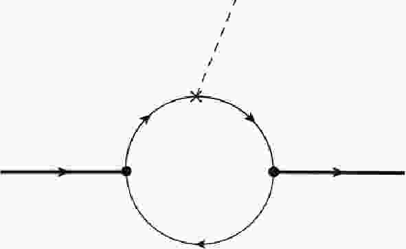
To maintain manifest covariance and explore the zero-mode effects, a CLF approach is presented in Refs. [9, 59, 60] with the help of a manifestly covariant BS approach as a guide to the calculation. In the CLF QM, the matrix element for
$ M'\to M'' $ transition is obtained by calculating the Feynman diagram shown in Fig. 1, and can be written as a manifest covariant form,
Figure 1. Feynman diagram for matrix element
$ \cal B $ in CLF QM.$ {\cal B}_{\rm {CLF}} = N_c \int \dfrac{{{\rm{d}}}^4 k_1'}{(2\pi)^4} \dfrac{H_{M'}H_{M''}}{N_1'\,N_1''\,N_2}iS\cdot (E_{M'}\, E_{M''}^*)\,, $

(32) where
$ {{\rm{d}}}^4 k_1' = \dfrac{1}{2} {{\rm{d}}} k_1'^- {{\rm{d}}} k_1'^+ {{\rm{d}}}^2 {\bf k}_{\bot}' $ ,$ E_{P,S} = 1 $ , and$ E_{V,A} = \epsilon_\mu $ , the denominators$ N_{1}^{(\prime,\prime\prime)} = k_{1}^{(\prime,\prime\prime)2}-m_1^{(\prime,\prime\prime)2}+i\epsilon $ and$ N_{2} = k_{2}^{2}- $ $m_2^{2}+i\epsilon $ come from the fermion propagators, and$ H_{M', M''} $ are vertex functions. The trace term S related to the fermion loop is written as$ S = {\rm {Tr}}\left[\Gamma\, (\not\!k'_1+m'_1)\,(i\Gamma_{M'})\,(-\!\not\!k_2+m_2)\,(i\gamma^0{\Gamma}_{M''}^{\dagger}\gamma^0) (\not\!k_1''+m_1'')\right]\,, $

(33) where
$ \Gamma_{M^{(\prime,\prime\prime)}} $ is the vertex operator and can be written as [9, 60, 84]$ i\Gamma_P = -i\gamma_5\,, $

(34) $ i\Gamma_S = -i\,, $

(35) $ i\Gamma_V = i\left[\gamma^\mu-\dfrac{ (k_1-k_2)^\mu}{D_{ V,{\rm {con}}}}\right]\,, $

(36) $ i\Gamma_{^1\!{A}} = i\dfrac{(k_1-k_2)^\mu}{D_{1,{\rm {con}}}}\gamma_5\,, $

(37) $ i\Gamma_{^3\!{A}} = i\left[\gamma^\mu+\dfrac{(k_1-k_2)^\mu}{D_{3,{\rm {con}}}}\right]\gamma_5\,, $

(38) with the constant forms of D factors,
$ D_{ (V,1,3),{\rm {con}}} =$ $ (M+m_1+m_2,\,2,\,M^2/(m_1-m_2)) $ .Integrating out the minus component of loop momentum, the covariant calculation becomes the LF calculation. By closing the contour in the upper complex
$ k_1'^- $ plane and assuming that$ H_{M', M''} $ are analytic within the contour, the integration picks up a residue at$ k_2^2 = \hat{k}_2^2 = m_2^2 $ corresponding to placement of the spectator antiquark on its mass-shell. Consequently, integrating out the minus component, one has the following replacements [9, 60]$ N_1 \to \hat{N}_1 = x \left(M^2-M_0^2\right) $

(39) and
$ \chi_M \equiv H_M/N\to h_M/\hat{N}\,,\quad D_{\rm {con}} \to D_{\rm {LF}}\,,\quad {({\rm{type-I}})} $

(40) where the LF forms of vertex functions,
$ h_M $ , for P, S, V, and A mesons are given by$ h_P/\hat{N} = h_V/\hat{N} = \dfrac{1}{\sqrt{2N_c}}\sqrt{\dfrac{\bar{x}}{x}}\dfrac{\psi_s}{\hat{M}_0}\,, $

(41) $ h_S/\hat{N} = \dfrac{1}{\sqrt{2N_c}}\sqrt{\dfrac{\bar{x}}{x}}\dfrac{\hat M'^2_0}{2\sqrt3M'_0}\dfrac{\psi_p}{\hat{M}_0}\,, $

(42) $ h_{^1\!{A}}/\hat{N} = \dfrac{1}{\sqrt{2N_c}}\sqrt{\dfrac{\bar{x}}{x}}\dfrac{\psi_p}{\hat{M}_0}\,, $

(43) $ h_{^3\!{A}}/\hat{N} = \dfrac{1}{\sqrt{2N_c}}\sqrt{\dfrac{\bar{x}}{x}}\dfrac{\hat M'^2_0}{2\sqrt2M'_0}\dfrac{\psi_p}{\hat{M}_0}\,. $

(44) As has aforementioned, a manifestly covariant BS approach is employed as a guide for the CLF calculation. Eq. (40) shows the Type-I correspondence between the manifestly covariant and LF models. In this formula, the correspondence between
$ \chi $ and$ \psi $ can be clearly derived by matching the covariant expressions to the SLF ones via zero-mode independent$ f_P $ or$ f_{+}^{P\to P}(q^2) $ [9, 60]; however the validity of the correspondence for the D factor appearing in the vertex operator,$ D_{V, {\rm {con}}} \to D_{V,{\rm {LF}}} $ , has not yet been explicitly clarified [84], it limits the replacement$ M\to M_0 $ only in the D factors. It should be noted that the covariant and the SLF results for$ f_P $ and$ f_+^{P\to P} $ are very simple (no meson mass appears in their formulas), thus the Type-I correspondence is possibly incomplete, as some other possible correspondences are impossible to obtain directly by matching the covariant result for$ f_P $ or$ f_+^{P\to P} $ to the SLF one. The main difference between the results in the manifestly covariant and SLF models is that the former allows nonzero binding energy, whereas the later is obtained at the zero-binding-energy limit at one-loop approximation (i.e., M vs.$ M_0 $ ). Based on these facts, instead of the traditional Type-I correspondence, a significantly more generalized correspondence,①$ \chi_M \equiv H_M/N\to h_M/\hat{N}\,,\qquad M\to M_0\,,\qquad {({\rm{type-II}})} $

(45) is suggested by Choi et al. for the purpose of self-consistent results for
$ f_{V} $ [84] (one may refer to Refs. [84–87] for more discussions).After integrating out
$ k_1'^- $ , the matrix element, Eq. (32), can be reduced to the LF form$ \hat{\cal B}_{\rm {CLF}} = N_c \int \dfrac{{{\rm{d}}} x {{\rm{d}}}^2 {\bf k}_{\bot}'}{2(2\pi)^3}\dfrac{h_{M'}h_{M''}}{\bar{x} \hat{N}_1'\,\hat{N}_1''\,}\hat{S}\cdot (E_{M'}\, E_{M''}^*)\,. $

(46) Notably, the matrix element in the CLF approach,
$ {\cal B}_{\rm {CLF}} $ given by Eq. (32), receives spurious contributions proportional to the light-like vector$ \omega^\mu = (0,2,{\bf 0}_\bot) $ , and these undesired spurious contributions are expected to be cancelled out by the zero-mode contributions [9, 60]. The inclusion of the zero-mode contribution in practice amounts to some proper replacements for$ \hat{k}_1' $ and$ \hat{N}_2 $ in$ \hat{S} $ under integration [9]. In this study, we require$ \hat{k}_1'^{\mu} \to P^\mu A_1^{(1)}+q^\mu A_2^{(1)} \,, $

(47) $ \begin{split} &\hat{k}_1'^{\mu}\hat{k}_1'^{\nu} \to g^{\mu\nu}A_1^{(2)}+P^\mu P^\nu A_2^{(2)}+(P^\mu q^\nu+q^\mu P^\nu)A_3^{(2)}\\&\quad+q^\mu q^\nu A_4^{(2)} +\dfrac{P^\mu\omega^\nu+\omega^\mu P^\nu}{\omega\cdot P}B_1^{(2)}\,, \end{split} $

(48) $ \hat{k}_1'^{\mu}\hat{N}_2\to q^\mu\left(A_2^{(1)}Z_2+\dfrac{q\cdot P}{q^2}A_1^{(2)} \right) \,, $

(49) where A and
$ B $ functions are written as$ A_1^{(1)} = \dfrac{x}{2}\,,\quad A_2^{(1)} = \dfrac{x}{2} -\dfrac{{ \bf k}_\bot' \cdot { \bf q}_\bot }{q^2}\,; $

(50) $ \begin{split} A_1^{(2)}& = -{ \bf k}_\bot'^2 -\dfrac{({ \bf k}_\bot' \cdot { \bf q}_\bot)^2}{q^2}\,,\;\; A_2^{(2)} = \left(A_1^{(1)}\right)^2\,,\;\; A_3^{(2)} = A_1^{(1)}A_2^{(1)}\,,\\ A_4^{(2)}& = \left(A_2^{(1)}\right)^2-\dfrac{1}{q^2}A_1^{(2)}\,,\;\; B_1^{(2)} = \dfrac{x}{2}Z_2-A_1^{(2)}\,;\\[-15pt] \end{split} $

(51) $ Z_2 = \hat{N}_1'+m_1'^2-m_2^2+(\bar{x}-x)M'^2+\left(q^2+q\cdot P\right)\frac{{ \bf k}_\bot' \cdot { \bf q}_\bot}{q^2}\,. $

(52) Here, we clarify that three types of terms appear in the decomposition of
$ \hat{k}_1'^{\mu} $ ,$ \hat{k}_1'^{\mu}\hat{k}_1'^{\nu} $ , etc., and are usually characterized by A, B, and C functions, respectively. The terms associated with A functions are$ \omega $ -independent, which can be clearly seen from Eqs. (47)–(49); the main$ \omega $ -dependent terms are associated with C functions, while these contributions are exactly eliminated by the inclusion of zero-mode contributions [9], and thus are not shown in Eqs. (47) and (48) for simplicity (one may refer to Ref. [9] for further detail); however, there are still some residual$ \omega $ -dependent, zero-mode independent, terms, which are associated with the B functions [9] (for instance, the last term in Eq. (48)). These residual$ \omega $ -dependent contributions possibly result in the covariance and self-consistence problems; however, they are not fully considered in some of the previous studies based on the CLF QM.In the CLF QM, the tensor form factors are obtained directly by matching
$ \hat{\cal B}_{\rm {CLF}} $ to their definitions given by Eqs. (1), (2), and (5)–(8)②. Our final CLF results for the tensor form factors can be written as$ [{\cal F}(q^2)]_{\rm {CLF}} = N_c\int\dfrac{{{\rm{d}}} x{{\rm{d}}}^2{\bf k'_\bot}}{2(2\pi)^3}\dfrac{\chi_{M'}\chi_{M''}}{\bar x}{\cal \widetilde{\cal F}}^{\rm {CLF}}(x,{\bf k'_\bot},q^2)\,, $

(53) where the integrands are
$ \widetilde{F}_T^{\rm{CLF}} = 2(M'+M'')\left[m'_1-(m'_1+m''_1-2m_2)A^{(1)}_1-(m'_1-m''_1)A^{(1)}_2\right]\,; $

(54) $ \widetilde{U}_T^{\rm {CLF}} = \widetilde{F}_T^{\rm{CLF}}[m''_1\rightarrow-m''_1]\,; $

(55) $ \begin{split}\quad\quad \widetilde{T}_1^{\rm {CLF}} = &\left(2\bar x-1\right)\left(m'^2_1+\hat N'_1\right)+m''^2_1+\hat N''_1+{ \bf q}_\bot^2+2\left(\bar xm'_1m''_1+xm'_1m_2+xm''_1m_2\right)-8A^{(2)}_1+2\left(M'^2-M''^2\right)\left(A^{(1)}_1+2A^{(2)}_2-2A^{(2)}_3\right)\\ &+2{ \bf q}_\bot^2\left(A^{(1)}_1-2A^{(1)}_2-2A^{(2)}_3+2A^{(2)}_4\right)-\frac{4}{D''_{V,{\rm {con}}}}(m'_1+m''_1)A^{(2)}_1\,, \end{split} $

(56) $ \begin{split}\quad\quad \widetilde{T}_2^{\rm {CLF}} = &-(m'_1-m''_1)^2-\hat N'_1-\hat N''_1+\bar xq^2+x\left[M'^2+M''^2+2(m'_1-m_2)(m_2-m''_1)\right]-\frac{q^2}{M'^2-M''^2}\bigg\{ 2M'^2+(m''_1-m'_1)^2\\ &-2(m'_1-m_2)^2-\hat N'_1+\hat N''_1-q^2-2Z_2+4Z_2A^{(1)}_2-4A^{(2)}_1-2\left[M'^2+M''^2-q^2+2(m'_1-m_2)(m_2-m''_1)\right]A^{(1)}_2\bigg\}\\ &-\frac{4}{D''_{V,{\rm {con}}}}A^{(2)}_1\left[m'_1+m''_1+\frac{{ \bf q}_\bot^2}{M'^2-M''^2}(m'_1-m''_1-2m_2)\right]\,, \end{split} $

(57) $ \begin{split}\quad\quad \widetilde{T}_3^{\rm {CLF}} = &2M'^2-2(m'_1-m_2)^2+(m'_1-m''_1)^2-\hat N'_1+\hat N''_1-q^2-2Z_2-4A^{(2)}_1+4\left(M'^2-M''^2\right)\left(A^{(1)}_1-A^{(2)}_2+A^{(2)}_4\right)\\ &+\dfrac{4\left(M'^2-M''^2\right)}{q^2}A^{(2)}_1+2\left[M''^2-3M'^2+q^2+2Z_2+2(m'_1-m_2)(m''_1-m_2)\right]A^{(1)}_2\\ &+\dfrac{4}{D''_{V,{\rm {con}}}}\times\bigg\{\left(M'^2-M''^2\right)\Big[m'_1\left(2A^{(1)}_1+2A^{(1)}_2-A^{(2)}_2-2A^{(2)}_3-A^{(2)}_4-1\right)\\ &-m''_1\left(A^{(1)}_1-A^{(1)}_2-A^{(2)}_2+A^{(2)}_4\right)-2m_2\left(A^{(1)}_1-A^{(2)}_2-A^{(2)}_3\right)\Big]+(m''_1-m'_1+2m_2)A^{(2)}_1\bigg\}\,; \end{split} $

(58) $ \widetilde{T}_{1,2,3}^{(1)\,,\rm{CLF}} = \widetilde{T}_{1,2,3}^{\rm {CLF}}\left[{D''-{\rm{terms}}\; {\rm{only}}}\,, D''_{V,{\rm {con}}}\to D''_{1,{\rm {con}}}\,,m''_1\rightarrow-m''_1\right]\,; $

(59) $ \widetilde{T}_{1,2,3}^{(3)\,,\rm{CLF}} = \widetilde{T}_{1,2,3}^{\rm {CLF}}[D''_{V,{\rm {con}}}\to D''_{3,{\rm {con}}}\,,m''_1\rightarrow-m''_1]\,. $

(60) Similar to the case of SLF results, only the
$ D'' $ -terms are kept in$ \widetilde{\cal T}_{1,2,3}^{(1)\,,\rm{ CLF}} $ , and the replacement$ m''_1\to-m''_1 $ must not be applied to the$ m''_1 $ in$ D'' $ factors. The CLF results Eqs. (53)–(60) are given in a general form, and the results within Type-I and -II correspondence schemes can be easily obtained by applying Eq. (40) and Eq. (45), respectively. Notably, the$ \omega $ -dependent contributions associated with B functions are not included in the results given above. These contributions lead to the self-consistence and covariance problems, and they are given and analyzed separately in the following section. Comparing our results for the$ P\to V\; (A) $ transition, Eqs. (56)–(58), with the ones obtained in the previous studies [81, 82], Eqs. (91)–(93), which are summarized in Appendix A, we find that our result for$ \widetilde{T}_1^{\rm {CLF}} $ , Eq. (56), is exactly the same as the one in Refs. [81, 82], Eq. (91); however, the results for$ \widetilde{T}_{2,3}^{\rm {CLF}} $ are different. This inconsistency will be analyzed in detail in the following section.In the CLF QM, for a given quantity (
$ \cal Q $ ), the CLF result ($ {\cal Q}^{\rm {CLF}} $ ) can be expressed as a sum of valence ($ {\cal Q}^{\rm {val.}} $ ) and zero-mode ($ {\cal Q}^{\rm {z.m.}} $ ) contributions [84],${\cal Q}^{\rm {CLF}} = {\cal Q}^{\rm {val.}}+ $ $ {\cal Q}^{\rm {z.m.}} $ , where the CLF results for the tensor form factors has been given above. Ref. [84] and our previous studies [85, 86] claim that$ {\cal Q}^{\rm {CLF}}\dot{ = }{\cal Q}^{\rm {val.}} = {\cal Q}^{\rm {SLF}} $ within the Type-II correspondence scheme, where “$ \dot{ = } $ ” denotes that two quantities are equal to each other only in numerical value, while “$ = $ ” indicates that two quantities are exactly the same, not only in numerical value, but also in form. To check the universality of such relation and clearly show the effects of zero-mode contributions, we have also calculated the valence contributions, which are written as$ \widetilde{F}_T^{\rm{val.}} = \widetilde{F}_T^{\rm{CLF}}\,; $

(61) $ \widetilde{U}_T^{\rm {val.}} = \widetilde{U}_T^{\rm{CLF}}\,; $

(62) $ \begin{split} \quad\quad \widetilde{T}_1^{\rm {val.}} = &\frac{1}{\bar x\left(M'^2-M''^2+{ \bf q}_\bot^2\right)}\bigg\{-2{ \bf k}_\bot'\cdot{ \bf q}_\bot{ \bf k}_\bot''^2+{ \bf k}_\bot'\cdot{ \bf k}_\bot''{ \bf q}_\bot^2-\bar x(2x-1){ \bf k}_\bot''\cdot{ \bf q}_\bot M'^2+2x(M'^2-M''^2)({ \bf k}_\bot'\cdot{ \bf k}_\bot''+m^2_2)\\ &+{ \bf k}_\bot'\cdot{ \bf q}_\bot(\bar xM''^2-2m^2_2)+2\bar x\left[m'_1m''_1-x(m'_1-m_2)(m''_1-m_2)\right](M'^2-M''^2+{ \bf q}_\bot^2)+m^2_2{ \bf q}_\bot^2\\ &+\frac{2}{D''_{V,{\rm {con}}}}(m'_1+m''_1)\Big[{ \bf k}_\bot'\cdot{ \bf q}_\bot{ \bf k}_\bot''^2+{ \bf k}_\bot''\cdot{ \bf q}_\bot(m^2_2-\bar x^2M'^2)+\bar x{ \bf k}_\bot'\cdot{ \bf k}_\bot''(M'^2-M''^2)\Big]\bigg\}\,, \end{split} $

(63) $ \begin{split}\quad\quad \widetilde{T}_2^{\rm {val.}} = &\widetilde{T}_1^{\rm {val.}}-\frac{q^2}{\left(M'^2-M''^2\right)\left(M'^{2}-M''^{2}+{ \bf q}_\bot^2\right)}\frac{1}{\bar x}\Bigg\{2{ \bf k}_\bot'\cdot{ \bf k}_\bot''{ \bf k}_\bot'\cdot{ \bf q}_\bot-2\bar x{ \bf k}_\bot'\cdot{ \bf q}_\bot{ \bf k}_\bot''\cdot{ \bf q}_\bot+{ \bf k}_\bot'\cdot{ \bf k}_\bot''{ \bf q}_\bot^2+2{ \bf k}_\bot'\cdot{ \bf k}_\bot''[(1+\bar x)M'^2\\ &+xM''^2+2(m'_1-m_2)(m_2-m''_1)]+2{ \bf k}_\bot''\cdot{ \bf q}_\bot(m^2_2-\bar x^2M'^2)-2\bar x({ \bf k}_\bot'\cdot{ \bf q}_\bot+{ \bf k}_\bot''\cdot{ \bf q}_\bot)(m'_1-m_2)(m_2-m''_1)\\ &-\bar xM'^2{ \bf k}_\bot''\cdot{ \bf q}_\bot-3\bar xM''^2{ \bf k}_\bot'\cdot{ \bf q}_\bot+m^2_2{ \bf q}_\bot^2+2\bar xm_2(m'_1-m''_1)(M'^2-M''^2+{ \bf q}_\bot^2)+2(M'^2+M''^2)\\ &\times\left[\bar x^2(m'_1-m_2)(m''_1-m_2)+m^2_2\right]-4\bar x^2M'^2M''^2+4m^2_2(m'_1-m_2)(m_2-m''_1)+\frac{2}{D''_{V,{\rm {con}}}}(m'_1-m''_1-2m_2)\\ &\times\bigg[{ \bf k}_\bot'\cdot{ \bf q}_\bot{ \bf k}_\bot''^2+\bar x{ \bf k}_\bot'\cdot{ \bf k}_\bot''(M'^2-M''^2)+{ \bf k}_\bot''\cdot{ \bf q}_\bot(m^2_2-\bar x^2M'^2) \bigg]\Bigg\} \,, \end{split} $

(64) $ \begin{split} \quad\quad \widetilde{T}_3^{\rm {val.}} = &\frac{M'^{2}-M''^{2}}{q^2}\left[\widetilde{T}_1^{\rm {val.}}-\widetilde{T}_2^{\rm {val.}}\right]+\frac{2\left(M'^{2}-M''^{2}\right)}{\bar x\left(M'^{2}-M''^{2}+{ \bf q}_\bot^2\right){ \bf q}_\bot^2}\bigg\{(\bar x-x){ \bf k}_\bot'\cdot{ \bf k}_\bot''{ \bf q}_\bot^2-2{ \bf k}_\bot'\cdot{ \bf q}_\bot\cdot{ \bf k}_\bot''^2\\ &+\bar x(\bar x-x)M'^2{ \bf k}_\bot''\cdot{ \bf q}_\bot+{ \bf k}_\bot'\cdot{ \bf q}_\bot(\bar xM''^2-2m^2_2)+(\bar x-x)m^2_2{ \bf q}_\bot^2+\frac{2}{D''_{V,{\rm {con}}}}{ \bf k}_\bot''\cdot{ \bf q}_\bot\\ &\times\Big[(m'_1+m''_1)({ \bf k}_\bot'^2-2\bar x{ \bf k}_\bot'\cdot{ \bf q}_\bot+m^2_2)+\bar x(xm_2-\bar xm''_1)M'^2-\bar x(xm_2+\bar xm'_1)(M''^2-{ \bf q}_\bot^2) \Big]\bigg\}\,; \end{split} $

(65) $ \widetilde{T}_{1,2,3}^{(1)\,,\rm{val.}} =\widetilde{T}_{1,2,3}^{\rm {val.}}[{D''-{\rm{terms}}\; {\rm{only}}}\,, D''_{V,{\rm {con}}}\to D''_{1,{\rm {con}}}, m''_1\to-m''_1]\,; $

(66) $\widetilde{T}_{1,2,3}^{(3)\,,\rm{val.}} = \widetilde{T}_{1,2,3}^{\rm {val.}}[D''_{V,{\rm {con}}}\to D''_{3,{\rm {con}}}, m''_1\to -m''_1]\,. $

(67) Thus, the tensor form factors of
$ P\to (P,S) $ transitions are free from the zero-mode effects, while the ones of$ P\to (V,A) $ transitions are zero-mode dependent. -
Using the theoretical results given in the last section and input parameters summarized in Appendix B, we present our numerical results and discussions in this section. As mentioned above, most of the spurious
$ \omega $ -dependent contributions are neutralized by zero-mode contributions; however, there are still some residuals associated with B functions, which possibly violate the self-consistence and covariance of CLF QM, but are not taken into account in Eqs. (54)–(60) and are not considered in the previous studies [80–82] either. These residual$ \omega $ -dependent contributions to the tensor matrix elements of$ P\to V $ transition (l.h.s. of Eqs. (5) and (6)) can be written as$ [{\cal B}]_{ B} = N_c\int\frac{{{\rm{d}}} x{{\rm{d}}}^2{\bf k'_\bot}}{2(2\pi)^3}\frac{\chi_V'\chi_V''}{\bar x}{\cal \widetilde{\cal B}}_{ B} $

(68) where
$ \begin{split} \widetilde{\cal B}_B^\mu(\Gamma = \sigma^{\mu\nu}q_\nu) = &4\frac{B_1^{(2)}}{\omega\cdot P}\bigg[ -\epsilon^{\delta\nu\alpha\beta}P_\delta q_\nu\omega_\alpha\epsilon^*_{\beta} P^\mu +\epsilon^{\mu\nu\alpha\beta}P_\nu\omega_\alpha\epsilon^{*}_{\beta}\left(M'^2-M''^2\right)\\ &+\epsilon^{\mu\nu\alpha\beta}q_\nu\omega_\alpha\epsilon^{*}_\beta\left(M'^2-M''^2\right) -\epsilon^{\mu\nu\alpha\beta}P_\nu q_\alpha\omega_\beta(q\cdot \epsilon^*)\frac{m'_1+m''_1}{D_{V,{\rm {con}}}''}\bigg]\,, \end{split} $

(69) $ \begin{split} \widetilde{\cal B}_B^\mu(\Gamma = \sigma^{\mu\nu}\gamma_5q_\nu) = &4i\frac{B_1^{(2)}}{\omega\cdot P}\Bigg\{ -P^\mu(\omega\cdot\epsilon^*)q^2\left(1+\frac{m'_1-m''_1-2m_2}{D_{V,{\rm {con}}}''}\right)+q^\mu(\omega\cdot\epsilon^*)\left(M'^2-M''^2\right)\left(1+\frac{m'_1-m''_1-2m_2}{D_{V,{\rm {con}}}''}\right)\\ &-\omega^\mu(q\cdot\epsilon^*)\bigg[q^2\left(1+\frac{m'_1-m''_1-2m_2}{D_{V,{\rm {con}}}''}\right)+\left(M'^2-M''^2\right)\left(1+\frac{m'_1-m''_1}{D_{V,{\rm {con}}}''}\right)\bigg]\Bigg\}\,. \end{split} $

(70) $ \widetilde{B}_B^\mu = 0 $ for$ P\to (P,S) $ transitions, and$ \widetilde{B}_B^\mu $ for$ P\to A $ transitions can be obtained from the above results by the replacements similar to Eqs. (59) and (60). Taking the contributions associated with B functions into account, the full results for the tensor form factors in the CLF QM can be expressed as$ [{\cal F}]^{\rm {full}} = [{\cal F}]^{\rm {CLF}}+[{\cal F}]^{ B}\,. $

(71) Based on these formulas, we have following discussions and findings:
● In Eq. (69), the first term would introduce a spurious unphysical form factor, and thus is expected to vanish. Unfortunately, it is equal to zero for
$ \lambda = 0 $ , but it is nonzero for$ \lambda = \pm $ within the Type-I scheme. The last three terms provide additional contributions to$ T_1 $ ; these however are$ \lambda $ -dependent. Explicitly, these contributions to$ T_1 $ can be written as$ {{\widetilde T}_1}^B = \left\{ {\begin{array}{*{20}{l}} {\left[ - 2({{M'}^2} - {{M''}^2}) + ({{M'}^2} - {{M''}^2} + {\bf{q}}_ \bot ^2)\dfrac{{{m_{1'}} + {m_{1''}}}}{{{D_{V,{\rm{co}}{{\rm{n}}^{\prime \prime }}}}}}\right]\dfrac{1}{{{{M''}^2}}}B_1^{(2)} ,}&{\quad\qquad \lambda = 0}\\ {\left[2({{M'}^2} - {{M''}^2}) - {\bf{q}}_ \bot ^2\dfrac{{{m_{1'}} + {m_{1''}}}}{{{D_{V,{\rm{co}}{{\rm{n}}^{\prime \prime }}}}}}\right]\dfrac{2}{{{{M'}^2} - {{M''}^2} + {\bf{q}}_ \bot ^2}}B_1^{(2)} ,}&{\quad\qquad \lambda = + }\\ {\left[1 + \dfrac{{{m_{1'}} + {m_{1''}}}}{{{D_{V,{\rm{co}}{{\rm{n}}^{\prime \prime }}}}}}\right]\dfrac{{2{\bf{q}}_ \bot ^2}}{{{{M'}^2} - {{M''}^2} + {\bf{q}}_ \bot ^2}}B_1^{(2)} .}&{\qquad\quad \lambda = - } \end{array}} \right. $

(72) Further considering the fact that
$ [{\cal F}]^{\rm {CLF}} $ is independent of the choice of$ \lambda $ , it can be concluded that$ T_1 $ in the CLF QM would suffer from a problem of self-consistence,$ [T_1]^{\rm {full}}_{\lambda = 0}\neq [T_1]^{\rm {full}}_{\lambda = +}\neq [T_1]^{\rm {full}}_{\lambda = -} $ , except that$ [T_1]^{\rm B} $ vanishes numerically. To clearly show the contributions of B function in Type-I and II schemes, we take$ B_{c}\to D^* $ and$ D_{s}\to \phi $ transitions as examples, and list the numerical results of$ [T_1]^{\rm {full}}_{\lambda = 0,\pm} $ in Table 1; moreover, the dependence of$ \Delta_{B}(x) $ is defined as$ B_{c}\to D^* $ 

$ [T_1]^{\rm{SLF}} $ 

$ [T_1]^{\rm{val.}} $ 

$ [T_1]^{\rm {CLF}} $ 

$ [T_1]^{\rm {full}}_{\lambda=0} $ 

$ [T_1]^{\rm {full}}_{\lambda=+} $ 

$ [T_1]^{\rm {full}}_{\lambda=-} $ 

$ {\bf{q}}_\perp^2=0\,{{\rm {GeV}}^2} $ 

type-I $ 0.106 $ 

$ 0.106 $ 

$ 0.094 $ 

$ 0.118 $ 

$ 0.081 $ 

$ 0.094 $ 

type-II $ 0.106 $ 

$ 0.106 $ 

$ 0.106 $ 

$ 0.106 $ 

$ 0.106 $ 

$ 0.106 $ 

$ {\bf{q}}_\perp^2=4\,{{\rm {GeV}}^2} $ 

type-I $ 0.072 $ 

$ 0.072 $ 

$ 0.063 $ 

$ 0.079 $ 

$ 0.055 $ 

$ 0.062 $ 

type-II $ 0.073 $ 

$ 0.073 $ 

$ 0.073 $ 

$ 0.073 $ 

$ 0.073 $ 

$ 0.073 $ 

$ {\bf{q}}_\perp^2=9\,{{\rm {GeV}}^2} $ 

type-I $ 0.046 $ 

$ 0.045 $ 

$ 0.040 $ 

$ 0.049 $ 

$ 0.035 $ 

$ 0.038 $ 

type-II $ 0.047 $ 

$ 0.047 $ 

$ 0.047 $ 

$ 0.047 $ 

$ 0.047 $ 

$ 0.047 $ 

$ D_{s}\to \phi $ 

$ [T_1]^{\rm{SLF}} $ 

$ [T_1]^{\rm{val.}} $ 

$ [T_1]^{\rm {CLF}} $ 

$ [T_1]^{\rm {full}}_{\lambda=0} $ 

$ [T_1]^{\rm {full}}_{\lambda=+} $ 

$ [T_1]^{\rm {full}}_{\lambda=-} $ 

$ {\bf{q}}_\perp^2=0\,{{\rm {GeV}}^2} $ 

type-I $ 0.687 $ 

$ 0.687 $ 

$ 0.658 $ 

$ 0.681 $ 

$ 0.630 $ 

$ 0.658 $ 

type-II $ 0.687 $ 

$ 0.687 $ 

$ 0.687 $ 

$ 0.687 $ 

$ 0.687 $ 

$ 0.687 $ 

$ {\bf{q}}_\perp^2=0.5\,{{\rm {GeV}}^2} $ 

type-I $ 0.597 $ 

$ 0.593 $ 

$ 0.568 $ 

$ 0.589 $ 

$ 0.544 $ 

$ 0.564 $ 

type-II $ 0.598 $ 

$ 0.598 $ 

$ 0.598 $ 

$ 0.598 $ 

$ 0.598 $ 

$ 0.598 $ 

$ {\bf{q}}_\perp^2=1\,{{\rm {GeV}}^2} $ 

type-I $ 0.524 $ 

$ 0.517 $ 

$ 0.495 $ 

$ 0.513 $ 

$ 0.476 $ 

$ 0.488 $ 

type-II $ 0.526 $ 

$ 0.526 $ 

$ 0.526 $ 

$ 0.526 $ 

$ 0.526 $ 

$ 0.526 $ 

Table 1. Numerical results of
$ T_1({\bf{q}}^{2}_{\bot}) $ for$ B_{c}\to D^* $ transition at$ {\bf q}_{\bot}^2 = (0,4,9) \,{{\rm {GeV}}^2} $ and for$ D_{s}\to \phi $ transition at$ {\bf q}_{\bot}^2 = (0,0.5,1) \,{{\rm {GeV}}^2} $ .$ \Delta_{B}(x) \equiv \dfrac{{{\rm{d}}} [{\cal F}]^{\rm B}_{\lambda}}{ {{\rm{d}}} x} = N_c\int\dfrac{{{\rm{d}}}^2{\bf k'_\bot}}{2(2\pi)^3}\dfrac{\chi_V'\chi_V''}{\bar x} \widetilde {\cal F}^{ B}_{\lambda}\,, $

(73) where
$ {\cal F} = T_1 $ , on x are shown in Fig. 2. These results show the self-consistency is violated in the traditional Type-I scheme (i.e.,$[T_1]^{\rm {full}}_{\lambda = 0}\neq $ $ [T_1]^{\rm {full}}_{\lambda = +}\neq [T_1]^{\rm {full}}_{\lambda = -} $ in Type-I scheme) due to the nonzero contributions of the B function,$ [T_1]^{\rm B}_{\lambda = 0,\pm} = \int_0^1{{\rm{d}}} x \Delta_{B}(x) \neq 0 $ (Type-I), but can be recovered using the Type-II scheme due to$ [T_1]^{ B}_{\lambda = 0,\pm}\dot{ = }0 $ ③, i.e.,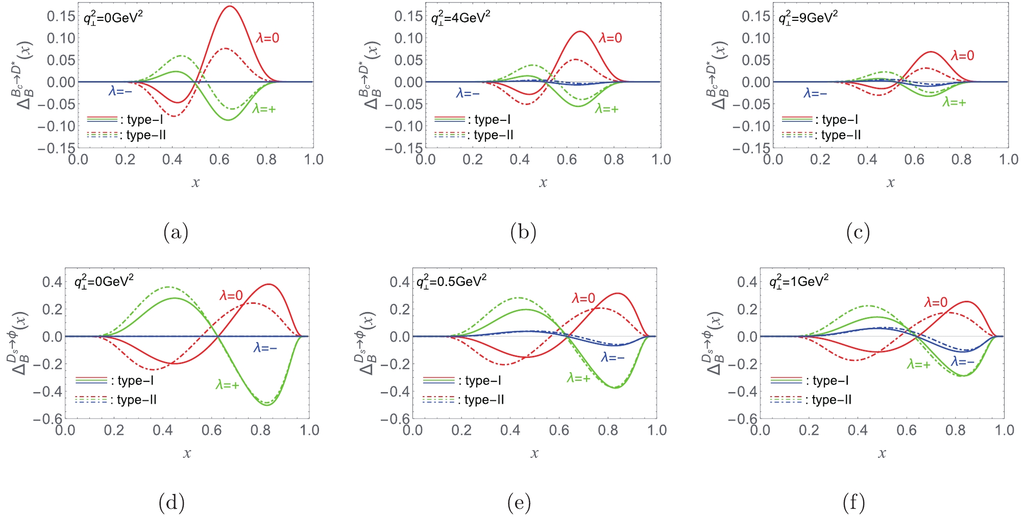
Figure 2. (color online) Dependences of
$ \Delta_{\rm B}(x) $ ($ {\cal F}=T_1 $ ) on x for$ B_{c}\to D^* $ transition at$ {\bf q}_{\bot}^2=(0,4,9)\,{{\rm {GeV}}^2} $ and for$ D_{s}\to \phi $ transition at$ {\bf q}_{\bot}^2=(0,0.5,1)\,{{\rm {GeV}}^2} $ .$ [T_1]^{\rm {full}}_{\lambda = 0}\dot{ = } [T_1]^{\rm {full}}_{\lambda = +}\dot{ = } [T_1]^{\rm {full}}_{\lambda = -}\,.\; \quad {({\rm{type-II}})} $

(74) ● In Eq. (70), the first and the second terms yield additional contributions to
$ T_2 $ and$ T_3 $ , the last term is proportional to$ \omega^\mu $ and corresponds to a unphysical form factor. We take$ T_3 $ as an example for convenience of discussion. The correction of the B function to$ T_3 $ is$ {\widetilde{T}_3}^{ B} = -4\dfrac{M'^2-M''^2}{ \epsilon^{*}\cdot q}\,\dfrac{\omega\cdot \epsilon^{*} }{\omega\cdot P}B_1^{(2)}\left(1+\frac{m_1'-m_1''-2m_2}{D_{V,{\rm {con}}}''}\right)\,, $

(75) which can be explicitly rewritten as a
$ \lambda $ -dependent form,$ {{\widetilde T}_3^{\rm{B}}} = \left\{ {\begin{split} &{ - 4\dfrac{{{{M'}^2}\! -\! {{M''}^2}}}{{{{M'}^2} \!-\! {{M''}^2}\! +\! q_ \bot ^2}}B_1^{(2)}\left( {1 + \dfrac{{{m_{1'}}\! -\! {m_{1''}}\! -\! 2{m_2}}}{{{D_{V,{\rm{co}}{{\rm{n}}^{\prime \prime }}}}}}} \right) , }\!&\!{\lambda = 0}\\ &{0. }\!&\!{\lambda = \pm } \end{split}} \right.$

(76) Compared with the B function contribution to the
$ A_3 $ for the$ V\to V $ transition,$ [{ \widetilde{A}_3}]^{\rm B} $ , given by Eqs. (4.5) and (4.6) in Ref. [87], it is found that$ [{ \widetilde{T}_3}]^{\rm B} = -{ [\widetilde{A}_3}]^{\rm B} $ . We have analyzed the effects of$ { [\widetilde{A}_3}]^{\rm B} $ ($ [{ \widetilde{T}_3}]^{\rm B} $ ) in Ref. [87] in detail and obtained the same conclusion as in the last item via$ T_1 $ .● The covariance of the matrix element of tensor operators in the Type-I scheme is violated due to the non-zero
$ \omega $ -dependent contributions associated with the B function (for instance, the last term proportional to$ \omega^\mu $ in Eq. (70)); meanwhile, the Lorentz covariance can be naturally recovered in the Type-II scheme, because all of the contributions associated with B function exist only in form but vanish numerically.● Taking
$ B_c\to D^* $ and$ D_s\to \phi $ transitions as examples once more, the numerical results of$ [ T_1]^{\rm {val.}} $ and$ [T_1]^{\rm {CLF}} $ are listed in Table 1, and the zero-mode contributions can be easily obtained via the relation$ [{\cal F}]^{\rm {CLF}} =[{\cal F}]^{\rm {val.}}+ $ $ [{\cal F}]^{\rm {z.m.}} $ . Further, the dependences of$ {{\rm{d}}} [{\cal F}]^{\rm {z.m.}}/{{\rm{d}}} x $ on x ($ {\cal F} = T_{1,2,3} $ ) are shown in Fig. 3. From Fig. 3 and Table 1, it can be found that the zero-mode effects are significant within the traditional type-I scheme; meanwhile, these contributions vanish numerically in the Type-II scheme, i.e.,$ [T_{1,2,3}(q^2)]_{\rm {z.m.}}\dot{ = } 0 $ (Type-II), which is similar to the case of B function contributions. Here, we would like to clarify that, the spurious$ \omega $ -dependent contributions associated with C functions have been neutralized by the zero-mode contributions [9], therefore the so-called zero-mode contribution ($ [{\cal F}]^{\rm {z.m.}} $ ) discussed above is from the residual zero-mode contribution to the matrix element. This implies that the zero-mode contributions to the matrix element within theType-II scheme are only responsible for neutralizing spurious$ \omega $ -dependent contributions associated with C functions, but do not contribute numerically to the form factors. There is no significant correlation between zero-mode and B function contributions found in both schemes, which can be clearly seen by comparing Fig. 2 with Fig. 3(a,d).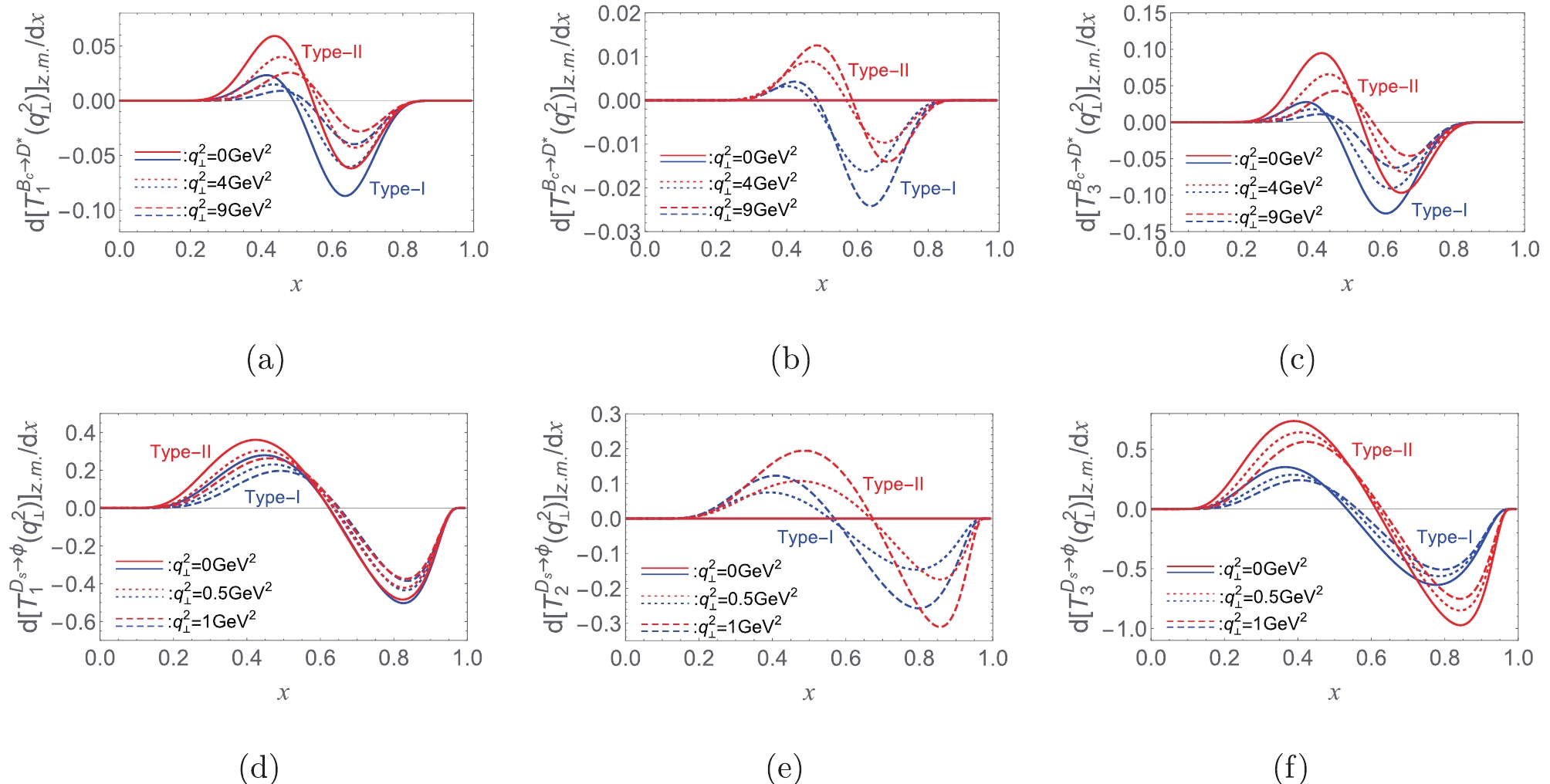
Figure 3. (color online) The dependences of
$ {{\rm{d}}} [T_{1,2,3}]_{\rm {z.m.}}/ {{\rm{d}}} x $ on x for$ B_{c}\to D^* $ transition at$ {\bf q}_{\bot}^2=(0,4,9)\,{{\rm {GeV}}^2} $ and for$ D_{s}\to \phi $ transition at$ {\bf q}_{\bot}^2=(0,0.5,1)\,{{\rm {GeV}}^2} $ .● Comparing
$ [T_{1,2,3}]^{\rm {SLF}} $ with$ [T_{1,2,3}]^{\rm val.} $ , which are given by Eqs. (28)–(29) and Eqs. (63)–(65), respectively, it can be found that the SLF results for$ T_{1,2,3} $ are exactly the same as the valence contributions in form after taking the$ M\to M_0 $ replacement (Type-II), which can also be clearly seen from the numerical results for$ T_1 $ in Table 1. This is exactly what we expect due to the following facts: (i) the CLF QM has employed the LF vertex functions, which can only be extracted by mapping the CLF result to the SLF one; (ii) the zero-mode contributions are not taken into account in the SLF result, therefore the SLF result is in fact only corresponding to the valence contribution in the CLF QM. The findings in this and last items can be concluded as$ [T_{1,2,3}]^{\rm {SLF}} = [T_{1,2,3}]^{\rm {val.}}\dot{ = }[T_{1,2,3}]^{\rm {CLF}}\,.\quad {({\rm{type-II}})} $

(77) This relation is also valid for the form factors of
$ P\to A $ and$ P\to (P,S) $ transitions, while, for the later, the notation “$ \dot{ = } $ ” should be replaced by “$ = $ ” because$ F_T $ and$ U_T $ are zero-mode independent.The analyses and findings mentioned above confirm again the main conclusion obtained in our previous studies [85, 86] and Ref. [84]. In addition to above-mentioned self-consistency problem of CLF QM caused by the contributions associated with B function, we note a new inconsistency problem, which is discussed in the following.
The tensor form factors
$ T_{1,2,3} $ have also been obtained by Cheng and Chua (CC) in Ref. [82] within the CLF QM, and their results are summarized in Appendix A (Eqs. (A1)–(A3)) for convenience of discussion. Comparing our results given by Eqs. (56)–(58) with CC's results, one can easily find that the results for$ T_1 $ are consistent with each other, whereas the ones for$ T_{2} $ and$ T_{3} $ are obviously different. In addition, for$ T_{2} $ and$ T_{3} $ , it is found that our and CC's numerical results are also inconsistent with each other in the traditional Type-I scheme. After carefully checking our and CC's calculations, we find that such new inconsistency problem is caused by the different approaches to deal with the trace term$ S^{\mu\nu\lambda} $ related to the fermion-loop in$ {\cal B}_{\rm {CLF}}^{P\to V}[\Gamma = \sigma^{\mu\nu}\gamma_5] $ , where$ {\cal B}_{\rm {CLF}} $ and S have been given by Eq. (32) and Eq. (33), respectively. Explicitly,$ {\cal B}_{\rm {CLF}}^{P\to V}[\Gamma = \sigma^{\mu\nu}\gamma_5] $ is written as$ {\cal B}_{\rm {CLF}}^{P\to V}[\Gamma = \sigma^{\mu\nu}\gamma_5] = N_c \int \frac{{{\rm{d}}}^4 k_1'}{(2\pi)^4} \frac{H_{P}H_{V}}{N_1'\,N_1''\,N_2}iS^{\mu\nu\lambda}\epsilon^*_\lambda \,. $

(78) The trace term,
$ S^{\mu\nu\lambda} $ , can be related to$ S'^{\rho\sigma\lambda} $ by using the identity$ 2\sigma_{\mu\nu}\gamma_5 = i\varepsilon_{\mu\nu\rho\sigma}\sigma^{\rho\sigma} $ , where$ S'^{\rho\sigma\lambda} $ is the trace term in$ {\cal B}_{\rm {CLF}}^{P\to V}[\Gamma = \sigma^{\rho\sigma}] $ corresponding to$ T_1 $ . Explicitly, it is written as$ S^{\mu\nu}_{\lambda} = \frac{i}{2}\varepsilon^{\mu\nu\rho\sigma} S'_{\rho\sigma\lambda} \qquad\qquad\qquad\qquad\qquad\qquad\qquad\qquad\qquad\qquad\qquad\qquad\;\;\qquad$

(79) $ \begin{split} = &i\varepsilon^{\mu\nu\rho\sigma}\bigg\{ \varepsilon_{\rho\sigma\lambda\alpha}\left[2(m'_1m_2+m''_1m_2-m'_1m''_1)k'^\alpha_1+m'_1m''_1P^{\alpha}+(m'_1m''_1-2m'_1m_2)q^{\alpha}\right]\\ &-\varepsilon_{\rho\sigma\alpha\beta}\frac{(4k'_{1}-3q-P)_\lambda}{D''_V}\left[(m'_1+m''_1)k'^{\alpha}_1P^\beta+(m''_1-m'_1+2m_2)k'^{\alpha}_1q^\beta+m'_1P^\alpha q^\beta\right]\\ &+\varepsilon_{\rho\sigma\lambda\alpha}\left[2(k'_1\cdot k_2-k''_1\cdot k_2-k'_1\cdot k''_1)k'^{\alpha}_1+k'_1\cdot k''_1P^\alpha+(k'_1\cdot k''_1-2k'_1\cdot k_2)q^\alpha\right]\\ &+(g^{\sigma}_{\lambda}\varepsilon_{\rho\alpha\beta\gamma}-g^{\rho}_{\lambda}\varepsilon_{\sigma\alpha\beta\gamma})P^{\alpha}q^{\beta}k'^{\gamma}_1+\varepsilon_{\sigma\rho\alpha\beta}(P^\alpha q^\beta k'_{1\lambda}+k'^\alpha_1P^\beta q_{\lambda}+q^\alpha k'^\beta_1P_{\lambda})\\ &+\varepsilon_{\rho\lambda\alpha\beta}\left[ k'_{1\sigma}P^\alpha q^\beta+q_\sigma P^\alpha k'^\beta_1 +(P+2q)_\sigma q^\alpha k'^\beta_1+2k'_{1\sigma} k'^\alpha_1 (P+q)^\beta \right]\\ &-\varepsilon_{\sigma\lambda\alpha\beta} \left[k'_{1\rho}P^\alpha q^\beta+q_\rho P^\alpha k'^\beta_1+(P+2q)_\rho q^\alpha k'^\beta_1+2k'_{1\rho}k'^\alpha_1(P+q)^\beta\right] \bigg\}\,. \end{split} $

(80) For convenience of discussion, we take the last term,
$ [S^{\mu\nu}_{\lambda}]_{{\rm{last}}\;{ \rm{term}}} = -2i\varepsilon^{\mu\nu\rho\sigma}\varepsilon_{\sigma\lambda\alpha\beta}\,k'_{1\rho}k'^\alpha_1(P+q)^\beta $ , as example.In the CC's calculation [82], the obtained result for
$ \hat{S}'_{\rho\sigma\lambda} $ is used directly to calculate$ \hat{S}^{\mu\nu}_{\lambda} $ using$ \hat{S}^{\mu\nu}_{\lambda} = \frac{i}{2}\varepsilon^{\mu\nu\rho\sigma} \hat{S}'_{\rho\sigma\lambda} $ , which is formally similar to Eq. (79). This implies that, after integrating out$ k'^-_{1} $ , the replacement for$ \hat{k}'^{\rho}_1\hat{k}'^\alpha_1 $ is made directly by using Eq. (48) even though$ \rho $ and$ \alpha $ are dummy indices; then, in the CC's approach, using the identity$ \begin{split} \varepsilon^{\mu\nu\rho\sigma}\varepsilon_{\sigma\lambda\alpha\beta} = &\left[g_\lambda^\mu(g_\alpha^\nu g_\beta^\rho-g_\alpha^\rho g_\beta^\nu)+g_\lambda^\nu(g_\alpha^\rho g_\beta^\mu-g_\alpha^\mu g_\beta^\rho)\right.\\ &\left.+g_\lambda^\rho(g_\alpha^\mu g_\beta^\nu-g_\alpha^\nu g_\beta^\mu)\right]\,, \end{split}$

(81) the following is obtained
$ \begin{split} \left[\hat{S}^{\mu\nu}_{\lambda}\right]_{{\rm{last}}\;{ \rm{term}}}^{\rm{CC}} = &2i g_\lambda^\nu g_\alpha^\mu g_\beta^\rho\left[g^\alpha_\rho A^{(2)}_1+P^\alpha P_\rho A^{(2)}_2+(P_\rho q^\alpha+q_\rho P^\alpha)A^{(2)}_3+q^\alpha q_\rho A^{(2)}_4\right](P+q)^\beta\,+\,...\\ = &2ig_\lambda^\nu\left\{P^\mu\left[A^{(2)}_1+(3M'^2-M''^2-q^2)A^{(2)}_2+(M'^2-M''^2+q^2)A^{(2)}_3\right]\right.\\ &\left.+q^\mu\left[A^{(2)}_1+\left(3M'^2-M''^2-q^2\right)A^{(2)}_3+\left(M'^2-M''^2+q^2\right)A^{(2)}_4\right] \right\}\,+\,...\,, \end{split} $

(82) where only the terms proportional to
$ g_\lambda^\nu g_\alpha^\mu g_\beta^\rho $ are shown for convenience of comparison with our corresponding result given in the following.In our calculation, we employ the standard procedure of the CLF calculation instead of directly using the obtained result for
$ \hat{S}'_{\rho\sigma\lambda} $ . First, we write$ [S^{\mu\nu}_{\lambda}]_{{\rm{last}}\;{ \rm{term}}} $ as$ \begin{split} \left[S^{\mu\nu}_{\lambda}\right]_{{\rm{last}}\;{ \rm{term}}}& = -2i g_\lambda^\nu k'^\mu_{1} k'_1\cdot(P+q)+...\\ & = -2i g_\lambda^\nu k'^\mu_{1} \left(M'^2+m'^2_1+m'^2_1-m^2_2- N_2 + N'_1 \right)+...\,, \end{split} $

(83) where only the terms proportional to
$ g_\lambda^\nu g_\alpha^\mu g_\beta^\rho $ corresponding to the CC' result, Eq. (82), are shown, by using Eq. (81) and$ k'_1\cdot q = \frac{1}{2}\left(N'_1+m'^2_1- N''_1-m''^2_1-{ \bf q}_\bot^2\right)\,, $

(84) $ k'_1\cdot P = \frac{1}{2}\left(2M'^2+ N'_1+m'^2_1+ N''_1+m''^2_1-2 N_2-2m^2_2+{ \bf q}_\bot^2\right)\,. $

(85) Then, after integrating out
$ k'^-_{1} $ , we further make replacements for$ \hat{k}_1'^\mu $ and$ \hat{k}_1'^\mu\hat{N}_2 $ (note that$ \mu $ is the free index) using Eqs. (47) and (49). Finally, we arrive at$ \begin{split} \left[\hat{S}^{\mu\nu}_{\lambda}\right]_{{\rm{last}}\;{ \rm{term}}}^{\rm{ours}} = &2ig_\lambda^\nu\Bigg\{P^\mu\left(M'^2+m'^2_1-m_2^2{+}\hat N'_1\right)A^{(1)}_1\\ &+q^\mu\left\Bigg[\left(M'^2+m'^2_1-m_2^2{+}\hat N'_1-Z_2\right)A^{(1)}_2\right.\\&\left.-\frac{M'^2-M''^2}{q^2}A^{(2)}_1\right\Bigg] \Bigg\}+...\,. \end{split} $

(86) Comparing CC's calculation with ours, it can be found that different replacements are required due to the different strategies for dealing with the S term, which further results in the different theoretical results for
$ \hat{S} $ , as well as for$ [T_2]^{\rm {CLF}} $ and$ [T_3]^{\rm {CLF}} $ . To clearly show the divergence between CC's results and ours, we take$ B_c\to D^* $ and$ D_s\to \phi $ transitions as examples, and plot the difference defined by$ \Delta^{\cal F}_{\rm {CLF}}(x,{ \bf q}_\bot^2)\equiv \frac{{{\rm{d}}} [{\cal F}]^{\rm {CLF}}_{\rm ours}}{{{\rm{d}}} x}-\frac{{{\rm{d}}} [{\cal F}]^{\rm {CLF}}_{\rm CC}}{{{\rm{d}}} x}\,, \;\; {\cal F} = T_2\;{\rm{ and }}\; T_3 $

(87) in Fig. 4. Fig. 4 shows that our and CC's numerical results for
$ [T_{2,3}]^{\rm {CLF}} $ are inconsistent with each other within the traditional Type-I scheme, because$ [T_{2,3}]^{\rm {CLF}}_{\rm ours}\! -\! [T_{2,3}]^{\rm {CLF}}_{\rm CC} \!= \int_0^1 {{\rm{d}}} x\,\Delta_{\rm {CLF}}^{T_{2,3}}(x)\neq 0 $ ; however, interestingly the consistency can be achieved numerically within the Type-II scheme, because$ \int_0^1 {{\rm{d}}} x\,\Delta_{\rm {CLF}}^{T_{2,3}}(x) = 0 $ . The case of$ P\to A $ transition is similar to the one of$ P\to V $ transition.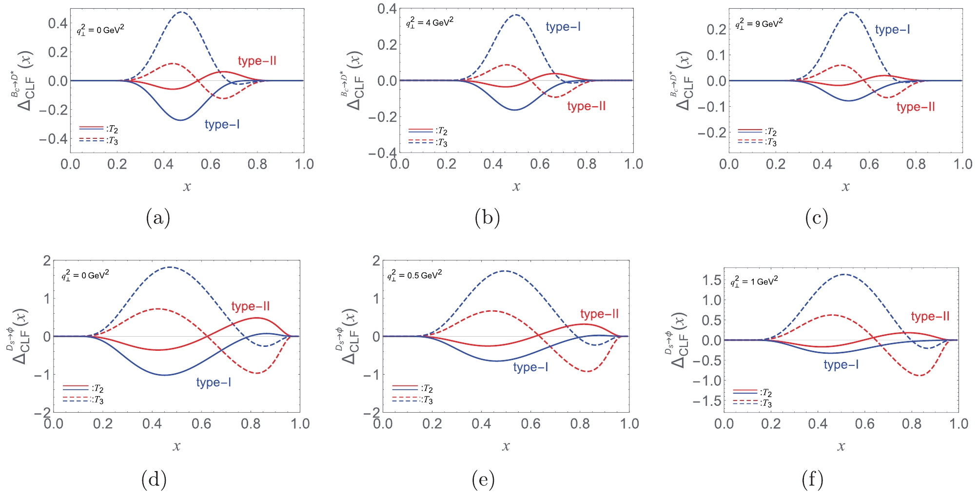
Figure 4. (color online)
$ \Delta^{T_{2,3}}_{\rm CLF}(x) $ for$ B_{c}\to D^* $ transition at$ {\bf q}_{\bot}^2=(0,4,9)\,{{\rm {GeV}}^2} $ and for$ D_{s}\to \phi $ transition at$ {\bf q}_{\bot}^2=(0,0.5,1)\,{{\rm {GeV}}^2} $ .From above analyses and discussions, it can be concluded that the Type-II scheme provides a feasible solution to the covariance and self-consistency problems of the CLF QM. Therefore, we update the CLF predictions for the tensor form factors of some
$ b\to c,\,s\,,q $ and$ c\to s,\,q $ ($ q = u,d $ ) induced$ P\to P,\,S,\,V $ , and A transitions by employing the self-consistent Type-II scheme. The CLF results for the tensor form factors are obtained in the$ q^+ = 0 $ frame, which implies that the form factors are known only for space-like momentum transfer,$ q^2 = -{\bf q}_\bot^2\leqslant 0 $ , and the results in the time-like region need an additional$ q^2 $ extrapolation. To achieve this purpose, the three parameters form [88]$ {\cal F}(q^2) = \dfrac{{\cal F}(0)}{1-a(q^2/M_{B,D}^2)+b(q^2/M_{B,D}^2)^2}\,, $

(88) is usually employed by the LFQMs. In Eq. (88),
$ M_{B,D} $ is the mass of the relevant B and D mesons, and$ M_{B_{q,s,c}} $ and$ M_{D_{q,s}} $ ($ q = u\,,d $ ) is used for$ b\to (q,s,c) $ and$ c\to (q,s) $ transitions, respectively; a and b are parameters obtained by fitting to the results computed directly by LFMQs. However, for the case of$ b\to $ light-quark transition with a heavy spectator quark, we find that the fitted results for b are very large, and some CLF results cannot be well reproduced using Eq. (88). Therefore, instead of Eq. (88), we employ an improved form [80]$ {\cal F}(q^2) = \dfrac{{\cal F}(0)}{\left( 1-q^2/M_{B,D}^2 \right)\left[1-a\left(q^2/M_{B,D}^2\right)+b\left(q^2/M_{B,D}^2\right)^2\right]}\,, $

(89) which is suitable for most of form factors considered in this study. However, for
$ T_3^{(1)} $ of some transitions, the coefficient b is rather sensitive to the range of$ q^2 $ . To overcome this difficulty, we fit$ T_3^{(1)} $ to the form [82]$ {\cal F}(q^2) = {\cal F}(0)\left[1+a\left(q^2/M_{B,D}^2\right)+b\left(q^2/M_{B,D}^2\right)^2\right]\,. $

(90) Using the values of input parameters collected in Appendix B, we then present our numerical predictions for the tensor form factors in Tables 2–6; and the
$ q^2 $ -dependences are shown in Figs. 5–9. From these results, it can be found that the CLF results obtained in the space-like region are well reproduced by Eqs. (89) and (90), and are further extrapolated to the time-like space. Further, our results for$ P\to V $ and A transitions respect the relation that$ T_1(0) = T_2(0) $ . These numerical results can be applied further in the relevant phenomenological studies of meson decays.$ {\cal{F}}(0) $ 

a b $ {\cal{F}}(0) $ 

a b $ F_T^{D\to \pi} $ 

$ 0.84^{+0.16}_{-0.13} $ 

$ -0.03^{+0.26}_{-0.18} $ 

$ 0.07^{+0.06}_{-0.09} $ 

$ F_T^{D_{s}\to K} $ 

$ 0.93^{+0.20}_{-0.15} $ 

$ -0.01^{+0.29}_{-0.20} $ 

$ 0.10^{+0.07}_{-0.10} $ 

$ F_T^{D\to K} $ 

$ 0.96^{+0.17}_{-0.15} $ 

$ -0.02^{+0.23}_{-0.23} $ 

$ 0.10^{+0.08}_{-0.10} $ 

$ F_T^{D_{s}\to \eta_{s}} $ 

$ 1.05^{+0.21}_{-0.17} $ 

$ 0.01^{+0.26}_{-0.20} $ 

$ 0.14^{+0.09}_{-0.11} $ 

$ F_T^{B\to \pi} $ 

$ 0.32^{+0.04}_{-0.04} $ 

$ 0.42^{+0.14}_{-0.10} $ 

$ 0.03^{+0.05}_{-0.06} $ 

$ F_T^{B_{s}\to K} $ 

$ 0.30^{+0.06}_{-0.06} $ 

$ 0.66^{+0.10}_{-0.08} $ 

$ 0.17^{+0.05}_{-0.06} $ 

$ F_T^{B_{c}\to D} $ 

$ 0.24^{+0.12}_{-0.10} $ 

$ 1.38^{+0.10}_{-0.11} $ 

$ 1.23^{+0.43}_{-0.42} $ 

$ F_T^{B\to K} $ 

$ 0.39^{+0.06}_{-0.05} $ 

$ 0.43^{+0.14}_{-0.10} $ 

$ 0.02^{+0.05}_{-0.06} $ 

$ F_T^{B_{s}\to \eta_{s}} $ 

$ 0.36^{+0.08}_{-0.07} $ 

$ 0.66^{+0.07}_{-0.05} $ 

$ 0.16^{+0.06}_{-0.07} $ 

$ F_T^{B_{c}\to D_{s}} $ 

$ 0.36^{+0.14}_{-0.12} $ 

$ 1.20^{+0.08}_{-0.09} $ 

$ 0.87^{+0.29}_{-0.30} $ 

$ F_T^{B\to D} $ 

$ 0.78^{+0.12}_{-0.12} $ 

$ 0.49^{+0.10}_{-0.10} $ 

$ -0.02^{+0.01}_{-0.01} $ 

$ F_T^{B_{s}\to D_{s}} $ 

$ 0.81^{+0.11}_{-0.14} $ 

$ 0.57^{+0.03}_{-0.02} $ 

$ 0.08^{+0.06}_{-0.06} $ 

$ F_T^{B_{c}\to \eta_{c}} $ 

$ 0.90^{+0.17}_{-0.22} $ 

$ 1.09^{+0.15}_{-0.20} $ 

$ 0.57^{+0.23}_{-0.23} $ 

Table 2. Numerical results of tensor form factors for
$ c\to q\,,s $ ($ q = u\,,d $ ) induced$ D_{q,s}\to P $ and$ b\to q\,,s\,,c $ induced$ B_{q,s,c}\to P $ transitions. Theoretical errors are caused by uncertainties of input parameters ($ \beta $ and$ m_{q,s,c,b} $ ).$ \mathcal{F}(0) $ 

a b $ \mathcal{F}(0) $ 

a b $ U_T^{D\to S_{(q,\bar{q})}} $ 

$ 0.77^{+0.13}_{-0.12} $ 

$ -0.17^{+0.26}_{-0.17} $ 

$ 0.18^{+0.11}_{-0.18} $ 

$ U_T^{D_{s}\to S_{(q,\bar{s})}} $ 

$ 0.94^{+0.17}_{-0.14} $ 

$ -0.16^{+0.26}_{-0.18} $ 

$ 0.17^{+0.09}_{-0.14} $ 

$ U_T^{D\to S_{(s,\bar{q})}} $ 

$ 0.74^{+0.13}_{-0.12} $ 

$ -0.17^{+0.25}_{-0.17} $ 

$ 0.16^{+0.11}_{-0.16} $ 

$ U_T^{D_{s}\to S_{(s,\bar{s})}} $ 

$ 0.93^{+0.16}_{-0.15} $ 

$ -0.18^{+0.26}_{-0.18} $ 

$ 0.20^{+0.11}_{-0.16} $ 

$ U_T^{B\to S_{(q,\bar{q})}} $ 

$ 0.35^{+0.05}_{-0.04} $ 

$ 0.28^{+0.21}_{-0.17} $ 

$ 0.02^{+0.04}_{-0.03} $ 

$ U_T^{B_{s}\to S_{(q,\bar{s})}} $ 

$ 0.38^{+0.04}_{-0.05} $ 

$ 0.47^{+0.08}_{-0.05} $ 

$ 0.12^{+0.05}_{-0.07} $ 

$ U_T^{B_{c}\to S_{(q,\bar{c})}} $ 

$ 0.40^{+0.13}_{-0.13} $ 

$ 1.16^{+0.18}_{-0.17} $ 

$ 0.88^{+0.38}_{-0.38} $ 

$ U_T^{B\to S_{(s,\bar{q})}} $ 

$ 0.37^{+0.05}_{-0.05} $ 

$ 0.25^{+0.19}_{-0.15} $ 

$ 0.01^{+0.03}_{-0.03} $ 

$ U_T^{B_{s}\to S_{(s,\bar{s})}} $ 

$ 0.43^{+0.06}_{-0.05} $ 

$ 0.44^{+0.26}_{-0.21} $ 

$ 0.11^{+0.05}_{-0.01} $ 

$ U_T^{B_{c}\to S_{(s,\bar{c})}} $ 

$ 0.56^{+0.12}_{-0.14} $ 

$ 0.98^{+0.10}_{-0.11} $ 

$ 0.62^{+0.24}_{-0.24} $ 

$ U_T^{B\to S_{(c,\bar{q})}} $ 

$ 0.51^{+0.09}_{-0.08} $ 

$ 0.33^{+0.12}_{-0.07} $ 

$ -0.08^{+0.04}_{-0.05} $ 

$ U_T^{B_{s}\to S_{(c,\bar{s})}} $ 

$ 0.71^{+0.12}_{-0.11} $ 

$ 0.36^{+0.11}_{-0.11} $ 

$ 0.03^{+0.01}_{-0.02} $ 

$ U_T^{B_{c}\to S_{(c,\bar{c})}} $ 

$ 1.21^{+0.32}_{-0.25} $ 

$ 0.83^{+0.35}_{-0.31} $ 

$ 0.40^{+0.30}_{-0.16} $ 

Table 3. Same as Table 2 except for
$ D_{q,s}\to S $ and$ B_{q,s,c}\to S $ transitions.$ \mathcal{F}(0) $ 

a b $ \mathcal{F}(0) $ 

a b $ T_1^{D\to\rho} $ 

$ 0.62_{-0.08}^{+0.08} $ 

$ 0.05_{-0.18}^{+0.26} $ 

$ 0.10_{-0.15}^{+0.08} $ 

$ T_1^{D_{s}\to K^*} $ 

$ 0.56_{-0.09}^{+0.09} $ 

$ 0.15^{+0.23}_{-0.16} $ 

$ 0.11^{+0.09}_{-0.13} $ 

$ T_2^{D\to\rho} $ 

$ 0.62_{-0.08}^{+0.08} $ 

$ -0.81^{+0.05}_{-0.05} $ 

$ 0.59^{+0.03}_{-0.03} $ 

$ T_2^{D_{s}\to K^*} $ 

$ 0.56_{-0.09}^{+0.09} $ 

$ -0.64^{+0.05}_{-0.15} $ 

$ 0.47^{+0.03}_{-0.03} $ 

$ T_3^{D\to\rho} $ 

$ 0.30^{+0.02}_{-0.02} $ 

$ -0.11^{+0.26}_{-0.16} $ 

$ 0.15^{+0.11}_{-0.18} $ 

$ T_3^{D_{s}\to K^*} $ 

$ 0.23_{-0.03}^{+0.02} $ 

$ -0.02^{+0.33}_{-0.12} $ 

$ 0.15^{+0.04}_{-0.15} $ 

$ T_1^{D\to K^*} $ 

$ 0.71_{-0.09}^{+0.08} $ 

$ 0.07^{+0.20}_{-0.15} $ 

$ 0.11^{+0.09}_{-0.12} $ 

$ T_1^{D_{s}\to \phi} $ 

$ 0.69_{-0.10}^{+0.08} $ 

$ 0.11^{+0.17}_{-0.13} $ 

$ 0.13^{+0.08}_{-0.08} $ 

$ T_2^{D\to K^*} $ 

$ 0.71_{-0.09}^{+0.08} $ 

$ -0.74^{+0.06}_{-0.06} $ 

$ 0.55^{+0.16}_{-0.16} $ 

$ T_2^{D_{s}\to \phi} $ 

$ 0.69_{-0.10}^{+0.08} $ 

$ -0.69^{+0.07}_{-0.07} $ 

$ 0.48^{+0.02}_{-0.02} $ 

$ T_3^{D\to K^*} $ 

$ 0.28_{-0.06}^{+0.03} $ 

$ -0.08^{+0.19}_{-0.18} $ 

$ 0.15^{+0.11}_{-0.10} $ 

$ T_3^{D_{s}\to \phi} $ 

$ 0.23_{-0.07}^{+0.03} $ 

$ -0.03^{+0.21}_{-0.20} $ 

$ 0.17^{+0.10}_{-0.09} $ 

$ T_1^{B\to \rho} $ 

$ 0.27_{-0.04}^{+0.05} $ 

$ 0.55^{+0.14}_{-0.09} $ 

$ 0.06^{+0.05}_{-0.06} $ 

$ T_1^{B_{s}\to K^{*}} $ 

$ 0.19_{-0.05}^{+0.06} $ 

$ 0.90^{+0.11}_{-0.09} $ 

$ 0.33^{+0.07}_{-0.08} $ 

$ T_2^{B\to \rho} $ 

$ 0.27_{-0.04}^{+0.05} $ 

$ -0.29^{+0.01}_{-0.01} $ 

$ 0.19^{+0.02}_{-0.03} $ 

$ T_2^{B_{s}\to K^{*}} $ 

$ 0.19_{-0.05}^{+0.06} $ 

$ 0.10^{+0.06}_{-0.06} $ 

$ 0.18^{+0.03}_{-0.04} $ 

$ T_3^{B\to \rho} $ 

$ 0.18_{-0.03}^{+0.03} $ 

$ 0.35^{+0.11}_{-0.07} $ 

$ 0.09^{+0.03}_{-0.06} $ 

$ T_3^{B_{s}\to K^{*}} $ 

$ 0.12_{-0.03}^{+0.03} $ 

$ 0.69^{+0.08}_{-0.07} $ 

$ 0.28^{+0.07}_{-0.07} $ 

$ T_1^{B_{c}\to D^{*}} $ 

$ 0.11_{-0.04}^{+0.06} $ 

$ 1.68^{+0.12}_{-0.12} $ 

$ 1.85^{+0.57}_{-0.57} $ 

$ T_1^{B\to K^{*}} $ 

$ 0.32_{-0.06}^{+0.06} $ 

$ 0.56^{+0.12}_{-0.09} $ 

$ 0.06^{+0.05}_{-0.06} $ 

$ T_2^{B_{c}\to D^{*}} $ 

$ 0.11_{-0.04}^{+0.06} $ 

$ 1.03^{+0.19}_{-0.23} $ 

$ 0.94^{+0.43}_{-0.38} $ 

$ T_2^{B\to K^{*}} $ 

$ 0.32_{-0.06}^{+0.06} $ 

$ -0.24^{+0.01}_{-0.01} $ 

$ 0.16^{+0.02}_{-0.03} $ 

$ T_3^{B_{c}\to D^{*}} $ 

$ 0.05_{-0.02}^{+0.03} $ 

$ 1.46^{+0.27}_{-0.17} $ 

$ 1.51^{+0.35}_{-0.52} $ 

$ T_3^{B\to K^{*}} $ 

$ 0.20_{-0.03}^{+0.03} $ 

$ 0.40^{+0.10}_{-0.07} $ 

$ 0.08^{+0.04}_{-0.06} $ 

$ T_1^{B_{s}\to\phi} $ 

$ 0.27_{-0.06}^{+0.07} $ 

$ 0.82^{+0.09}_{-0.07} $ 

$ 0.26^{+0.06}_{-0.07} $ 

$ T_1^{B_{c}\to D^{*}_{s}} $ 

$ 0.20_{-0.07}^{+0.09} $ 

$ 1.34^{+0.11}_{-0.11} $ 

$ 1.06^{+0.34}_{-0.34} $ 

$ T_2^{B_{s}\to\phi} $ 

$ 0.27_{-0.06}^{+0.07} $ 

$ 0.05^{+0.04}_{-0.04} $ 

$ 0.16^{+0.03}_{-0.03} $ 

$ T_2^{B_{c}\to D^{*}_{s}} $ 

$ 0.20_{-0.07}^{+0.09} $ 

$ 0.63^{+0.17}_{-0.20} $ 

$ 0.49^{+0.22}_{-0.18} $ 

$ T_3^{B_{s}\to\phi} $ 

$ 0.16_{-0.03}^{+0.04} $ 

$ 0.64^{+0.07}_{-0.06} $ 

$ 0.23^{+0.05}_{-0.06} $ 

$ T_3^{B_{c}\to D^{*}_{s}} $ 

$ 0.10_{-0.03}^{+0.04} $ 

$ 1.16^{+0.10}_{-0.11} $ 

$ 0.87^{+0.30}_{-0.29} $ 

$ T_1^{B\to D^{*}} $ 

$ 0.70_{-0.11}^{+0.10} $ 

$ 0.55^{+0.04}_{-0.03} $ 

$ 0.00^{+0.05}_{-0.04} $ 

$ T_1^{B_{s}\to D^{*}_{s}} $ 

$ 0.70_{-0.12}^{+0.11} $ 

$ 0.63^{+0.10}_{-0.10} $ 

$ 0.10^{+0.06}_{-0.07} $ 

$ T_2^{B\to D^{*}} $ 

$ 0.70_{-0.11}^{+0.10} $ 

$ -0.28^{+0.01}_{-0.02} $ 

$ 0.19^{+0.03}_{-0.02} $ 

$ T_2^{B_{s}\to D^{*}_{s}} $ 

$ 0.70_{-0.12}^{+0.11} $ 

$ -0.22^{+0.07}_{-0.07} $ 

$ 0.24^{+0.02}_{-0.02} $ 

$ T_3^{B\to D^{*}} $ 

$ 0.30_{-0.03}^{+0.01} $ 

$ 0.42^{+0.08}_{-0.10} $ 

$ 0.02^{+0.02}_{-0.02} $ 

$ T_3^{B_{s}\to D^{*}_{s}} $ 

$ 0.30_{-0.02}^{+0.02} $ 

$ 0.54^{+0.01}_{-0.01} $ 

$ 0.06^{+0.01}_{-0.01} $ 

$ T_1^{B_{c}\to J/ \Psi} $ 

$ 0.56_{-0.17}^{+0.16} $ 

$ 1.30^{+0.17}_{-0.23} $ 

$ 0.80^{+0.31}_{-0.31} $ 

$ T_2^{B_{c}\to J/ \Psi} $ 

$ 0.56_{-0.17}^{+0.16} $ 

$ 0.54^{+0.20}_{-0.29} $ 

$ 0.34^{+0.16}_{-0.12} $ 

$ T_3^{B_{c}\to J/ \Psi} $ 

$ 0.19_{-0.03}^{+0.03} $ 

$ 1.17^{+0.03}_{-0.02} $ 

$ 0.68^{+0.17}_{-0.21} $ 

Table 4. Same as Table 2 except for
$ D_{q,s}\to V $ and$ B_{q,s,c}\to V $ transitions.$ \mathcal{F}(0) $ 

a b $ \mathcal{F}(0) $ 

a b $ T_1^{D\to {^1\!A}_{(q,\bar{q})}} $ 

$ 0.23^{+0.02}_{-0.03} $ 

$ 0.02^{+0.23}_{-0.14} $ 

$ 0.18^{+0.10}_{-0.15} $ 

$ T_1^{D_{s}\to {^1\!A}_{(q,\bar{s})}} $ 

$ 0.19^{+0.02}_{-0.03} $ 

$ 0.13^{+0.20}_{-0.20} $ 

$ 0.18^{+0.08}_{-0.14} $ 

$ T_2^{D\to {^1\!A}_{(q,\bar{q})}} $ 

$ 0.23^{+0.02}_{-0.03} $ 

$ -0.82^{+0.07}_{-0.13} $ 

$ 0.72^{+0.09}_{-0.06} $ 

$ T_2^{D_{s}\to {^1\!A}_{(q,\bar{s})}} $ 

$ 0.19^{+0.02}_{-0.03} $ 

$ -0.40^{+0.04}_{-0.04} $ 

$ 0.35^{+0.14}_{-0.14} $ 

$ T_3^{D\to {^1\!A}_{(q,\bar{q})}} $ 

$ -0.02^{+0.12}_{-0.09} $ 

$ 3.76^{+0.25}_{-0.25} $ 

$ 5.25^{+0.47}_{-0.47} $ 

$ T_3^{D_{s}\to {^1\!A}_{(q,\bar{s})}} $ 

$ -0.13^{+0.12}_{-0.06} $ 

$ 1.16^{+0.07}_{-0.07} $ 

$ 1.01^{+0.23}_{-0.23} $ 

$ T_1^{D\to {^1\!A}_{(s,\bar{q})}} $ 

$ 0.19^{+0.03}_{-0.04} $ 

$ 0.04^{+0.21}_{-0.21} $ 

$ 0.20^{+0.09}_{-0.09} $ 

$ T_1^{D_{s}\to {^1\!A}_{(s,\bar{s})}} $ 

$ 0.16^{+0.03}_{-0.03} $ 

$ 0.09^{+0.28}_{-0.22} $ 

$ 0.20^{+0.09}_{-0.08} $ 

$ T_2^{D\to {^1\!A}_{(s,\bar{q})}} $ 

$ 0.19^{+0.03}_{-0.04} $ 

$ -1.32^{+0.26}_{-0.40} $ 

$ 1.69^{+0.59}_{-0.59} $ 

$ T_2^{D_{s}\to {^1\!A}_{(s,\bar{s})}} $ 

$ 0.16^{+0.03}_{-0.03} $ 

$ -0.83^{+0.04}_{-0.20} $ 

$ 0.79^{+0.18}_{-0.06} $ 

$ T_3^{D\to {^1\!A}_{(s,\bar{q})}} $ 

$ 0.01^{+0.17}_{-0.11} $ 

$ -4.77^{+0.40}_{-0.40} $ 

$ -9.34^{+0.50}_{-0.49} $ 

$ T_3^{D_{s}\to {^1\!A}_{(s,\bar{s})}} $ 

$ -0.10^{+0.11}_{-0.11} $ 

$ 1.10^{+0.38}_{-0.38} $ 

$ 0.93^{+0.26}_{-0.26} $ 

$ T_1^{B\to {^1\!A}_{(q,\bar{q})}} $ 

$ 0.12^{+0.03}_{-0.03} $ 

$ 0.72^{+0.11}_{-0.08} $ 

$ 0.17^{+0.05}_{-0.05} $ 

$ T_1^{B_{s}\to {^1\!A}_{(q,\bar{s})}} $ 

$ 0.08^{+0.03}_{-0.03} $ 

$ 1.07^{+0.05}_{-0.05} $ 

$ 0.53^{+0.11}_{-0.10} $ 

$ T_2^{B\to {^1\!A}_{(q,\bar{q})}} $ 

$ 0.12^{+0.03}_{-0.03} $ 

$ -0.15^{+0.06}_{-0.08} $ 

$ 0.19^{+0.03}_{-0.03} $ 

$ T_2^{B_{s}\to {^1\!A}_{(q,\bar{s})}} $ 

$ 0.08^{+0.03}_{-0.03} $ 

$ 0.33^{+0.11}_{-0.13} $ 

$ 0.20^{+0.07}_{-0.03} $ 

$ T_3^{B\to {^1\!A}_{(q,\bar{q})}} $ 

$ -0.01^{+0.02}_{-0.03} $ 

$ 3.37^{+0.14}_{-0.14} $ 

$ 3.09^{+0.24}_{-0.24} $ 

$ T_3^{B_{s}\to {^1\!A}_{(q,\bar{s})}} $ 

$ -0.07^{+0.03}_{-0.03} $ 

$ 1.87^{+0.27}_{-0.22} $ 

$ 1.30^{+0.23}_{-0.23} $ 

$ T_1^{B_{c}\to {^1\!A}_{(q,\bar{c})}} $ 

$ 0.03^{+0.03}_{-0.01} $ 

$ 1.78^{+0.16}_{-0.16} $ 

$ 2.05^{+0.67}_{-0.67} $ 

$ T_1^{B\to {^1\!A}_{(s,\bar{q})}} $ 

$ 0.13^{+0.03}_{-0.03} $ 

$ 0.72^{+0.09}_{-0.06} $ 

$ 0.18^{+0.05}_{-0.06} $ 

$ T_2^{B_{c}\to {^1\!A}_{(q,\bar{c})}} $ 

$ 0.03^{+0.03}_{-0.01} $ 

$ 1.55^{+0.24}_{-0.28} $ 

$ 1.51^{+0.69}_{-0.69} $ 

$ T_2^{B\to {^1\!A}_{(s,\bar{q})}} $ 

$ 0.13^{+0.03}_{-0.03} $ 

$ -0.27^{+0.13}_{-0.13} $ 

$ 0.28^{+0.06}_{-0.05} $ 

$ T_3^{B_{c}\to {^1\!A}_{(q,\bar{c})}} $ 

$ -0.17^{+0.05}_{-0.03} $ 

$ 2.41^{+0.13}_{-0.13} $ 

$ 2.02^{+0.15}_{-0.16} $ 

$ T_3^{B\to {^1\!A}_{(s,\bar{q})}} $ 

$ -0.02^{+0.03}_{-0.04} $ 

$ 2.88^{+0.51}_{-0.51} $ 

$ 2.55^{+0.58}_{-0.58} $ 

$ T_1^{B_{s}\to {^1\!A}_{(s,\bar{s})}} $ 

$ 0.09^{+0.03}_{-0.02} $ 

$ 0.97^{+0.05}_{-0.03} $ 

$ 0.42^{+0.07}_{-0.07} $ 

$ T_1^{B_{c}\to {^1\!A}_{(s,\bar{c})}} $ 

$ 0.06^{+0.03}_{-0.03} $ 

$ 1.41^{+0.15}_{-0.14} $ 

$ 1.19^{+0.49}_{-0.40} $ 

$ T_2^{B_{s}\to {^1\!A}_{(s,\bar{s})}} $ 

$ 0.09^{+0.03}_{-0.02} $ 

$ 0.11^{+0.13}_{-0.16} $ 

$ 0.22^{+0.02}_{-0.02} $ 

$ T_2^{B_{c}\to {^1\!A}_{(s,\bar{c})}} $ 

$ 0.06^{+0.03}_{-0.03} $ 

$ 1.11^{+0.24}_{-0.27} $ 

$ 0.74^{+0.49}_{-0.38} $ 

$ T_3^{B_{s}\to {^1\!A}_{(s,\bar{s})}} $ 

$ -0.10^{+0.04}_{-0.04} $ 

$ 1.93^{+0.24}_{-0.18} $ 

$ 1.43^{+0.28}_{-0.21} $ 

$ T_3^{B_{c}\to {^1\!A}_{(s,\bar{c})}} $ 

$ -0.28^{+0.07}_{-0.10} $ 

$ 2.22^{+0.39}_{-0.37} $ 

$ 1.82^{+0.54}_{-0.47} $ 

$ T_1^{B\to {^1\!A}_{(c,\bar{q})}} $ 

$ 0.15^{+0.02}_{-0.02} $ 

$ 0.64^{+0.01}_{-0.01} $ 

$ 0.11^{+0.04}_{-0.03} $ 

$ T_1^{B_{s}\to {^1\!A}_{(c,\bar{s})}} $ 

$ 0.12^{+0.02}_{-0.01} $ 

$ 0.73^{+0.17}_{-0.13} $ 

$ 0.22^{+0.04}_{-0.05} $ 

$ T_2^{B\to {^1\!A}_{(c,\bar{q})}} $ 

$ 0.15^{+0.02}_{-0.02} $ 

$ -1.89^{+0.44}_{-0.65} $ 

$ 2.90^{+0.94}_{-0.94} $ 

$ T_2^{B_{s}\to {^1\!A}_{(c,\bar{s})}} $ 

$ 0.12^{+0.02}_{-0.01} $ 

$ -1.57^{+0.05}_{-0.05} $ 

$ 2.31^{+0.06}_{-0.06} $ 

$ T_3^{B\to {^1\!A}_{(c,\bar{q})}} $ 

$ -0.07^{+0.10}_{-0.06} $ 

$ 3.56^{+0.92}_{-0.92} $ 

$ 4.69^{+0.89}_{-0.89} $ 

$ T_3^{B_{s}\to {^1\!A}_{(c,\bar{s})}} $ 

$ -0.20^{+0.10}_{-0.06} $ 

$ 2.42^{+0.20}_{-0.20} $ 

$ 2.82^{+0.39}_{-0.39} $ 

$ T_1^{B_{c}\to {^1\!A}_{(c,\bar{c})}} $ 

$ 0.08^{+0.02}_{-0.02} $ 

$ 1.34^{+0.05}_{-0.04} $ 

$ 0.88^{+0.21}_{-0.21} $ 

$ T_2^{B_{c}\to {^1\!A}_{(c,\bar{c})}} $ 

$ 0.08^{+0.02}_{-0.02} $ 

$ 0.23^{+0.20}_{-0.21} $ 

$ 0.47^{+0.04}_{-0.04} $ 

$ T_3^{B_{c}\to {^1\!A}_{(c,\bar{c})}} $ 

$ -0.48^{+0.12}_{-0.11} $ 

$ 2.45^{+0.60}_{-0.60} $ 

$ 2.90^{+0.52}_{-0.52} $ 

Table 5. Same as Table 2 except for
$ D_{q,s} $ $ \to $ $ ^1\!A $ and$ B_{q,s,c} $ $ \to $ $ ^1\!A $ transitions.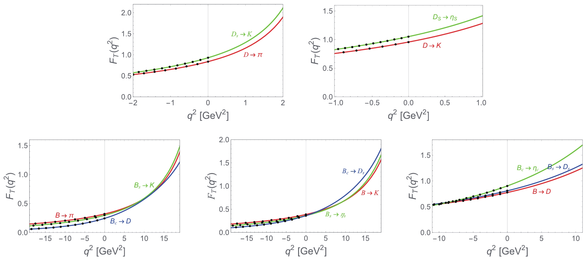
Figure 5. (color online)
$ q^2 $ dependences of tensor form factors for$ c\to q\,,s $ ($ q = u\,,d $ ) induced$ D_{q,s}\to P $ and$ b\to q\,,s\,,c $ induced$ B_{q,s,c}\to P $ transitions. Dots in the space-like region are the results obtained directly via the CLF QM, and the lines depict fitting results.$ {\cal{F}}(0) $ 

a b $ {\cal{F}}(0) $ 

a b $ T_1^{D\to {^3\!A}_{(q,\bar{q})}} $ 

$ 0.49^{+0.05}_{-0.04} $ 

$ -0.09^{+0.29}_{-0.21} $ 

$ 0.17^{+0.14}_{-0.18} $ 

$ T_1^{D_{s}\to {^3\!A}_{(q,\bar{s})}} $ 

$ 0.49^{+0.05}_{-0.05} $ 

$ -0.04^{+0.32}_{-0.22} $ 

$ 0.19^{+0.12}_{-0.17} $ 

$ T_2^{D\to {^3\!A}_{(q,\bar{q})}} $ 

$ 0.49^{+0.05}_{-0.04} $ 

$ -2.06^{+0.66}_{-0.66} $ 

$ 3.24^{+0.41}_{-0.41} $ 

$ T_2^{D_{s}\to {^3\!A}_{(q,\bar{s})}} $ 

$ 0.49^{+0.05}_{-0.05} $ 

$ -1.93^{+0.43}_{-0.66} $ 

$ 3.06^{+0.53}_{-0.53} $ 

$ T_3^{D\to {^3\!A}_{(q,\bar{q})}} $ 

$ 0.50^{+0.12}_{-0.10} $ 

$ -0.21^{+0.29}_{-0.21} $ 

$ 0.20^{+0.19}_{-0.18} $ 

$ T_3^{D_{s}\to {^3\!A}_{(q,\bar{s})}} $ 

$ 0.54^{+0.14}_{-0.11} $ 

$ -0.14^{+0.34}_{-0.24} $ 

$ 0.22^{+0.19}_{-0.19} $ 

$ T_1^{D\to {^3\!A}_{(s,\bar{q})}} $ 

$ 0.43^{+0.05}_{-0.07} $ 

$ -0.09^{+0.14}_{-0.13} $ 

$ 0.18^{+0.11}_{-0.11} $ 

$ T_1^{D_{s}\to {^3\!A}_{(s,\bar{s})}} $ 

$ 0.47^{+0.04}_{-0.06} $ 

$ -0.07^{+0.11}_{-0.10} $ 

$ 0.22^{+0.08}_{-0.10} $ 

$ T_2^{D\to {^3\!A}_{(s,\bar{q})}} $ 

$ 0.43^{+0.05}_{-0.07} $ 

$ -3.05^{+0.72}_{-0.72} $ 

$ 7.09^{+0.51}_{-0.51} $ 

$ T_2^{D_{s}\to {^3\!A}_{(s,\bar{s})}} $ 

$ 0.47^{+0.04}_{-0.06} $ 

$ -3.10^{+0.79}_{-0.79} $ 

$ 7.20^{+0.14}_{-0.14} $ 

$ T_3^{D\to {^3\!A}_{(s,\bar{q})}} $ 

$ 0.51^{+0.14}_{-0.13} $ 

$ -0.26^{+0.39}_{-0.27} $ 

$ 0.28^{+0.22}_{-0.29} $ 

$ T_3^{D_{s}\to {^3\!A}_{(s,\bar{s})}} $ 

$ 0.66^{+0.16}_{-0.13} $ 

$ -0.14^{+0.28}_{-0.22} $ 

$ 0.19^{+0.20}_{-0.11} $ 

$ T_1^{B\to {^3\!A}_{(q,\bar{q})}} $ 

$ 0.29^{+0.03}_{-0.03} $ 

$ 0.35^{+0.21}_{-0.20} $ 

$ 0.03^{+0.03}_{-0.02} $ 

$ T_1^{B_{s}\to {^3\!A}_{(q,\bar{s})}} $ 

$ 0.26^{+0.04}_{-0.06} $ 

$ 0.65^{+0.06}_{-0.04} $ 

$ 0.21^{+0.07}_{-0.09} $ 

$ T_2^{B\to {^3\!A}_{(q,\bar{q})}} $ 

$ 0.29^{+0.03}_{-0.03} $ 

$ -0.71^{+0.01}_{-0.01} $ 

$ 0.46^{+0.05}_{-0.02} $ 

$ T_2^{B_{s}\to {^3\!A}_{(q,\bar{s})}} $ 

$ 0.26^{+0.04}_{-0.06} $ 

$ -0.38^{+0.14}_{-0.16} $ 

$ 0.37^{+0.07}_{-0.05} $ 

$ T_3^{B\to {^3\!A}_{(q,\bar{q})}} $ 

$ 0.25^{+0.04}_{-0.03} $ 

$ 0.12^{+0.23}_{-0.18} $ 

$ 0.12^{+0.03}_{-0.02} $ 

$ T_3^{B_{s}\to {^3\!A}_{(q,\bar{s})}} $ 

$ 0.25^{+0.04}_{-0.05} $ 

$ 0.49^{+0.01}_{-0.01} $ 

$ 0.23^{+0.06}_{-0.07} $ 

$ T_1^{B_{c}\to {^3\!A}_{(q,\bar{c})}} $ 

$ 0.18^{+0.09}_{-0.07} $ 

$ 1.43^{+0.19}_{-0.21} $ 

$ 1.28^{+0.51}_{-0.51} $ 

$ T_1^{B\to {^3\!A}_{(s,\bar{q})}} $ 

$ 0.29^{+0.04}_{-0.03} $ 

$ 0.34^{+0.23}_{-0.19} $ 

$ 0.04^{+0.02}_{-0.02} $ 

$ T_2^{B_{c}\to {^3\!A}_{(q,\bar{c})}} $ 

$ 0.18^{+0.09}_{-0.07} $ 

$ 0.46^{+0.39}_{-0.44} $ 

$ 0.71^{+0.13}_{-0.13} $ 

$ T_2^{B\to {^3\!A}_{(s,\bar{q})}} $ 

$ 0.29^{+0.04}_{-0.03} $ 

$ -0.85^{+0.02}_{-0.04} $ 

$ 0.61^{+0.10}_{-0.07} $ 

$ T_3^{B_{c}\to {^3\!A}_{(q,\bar{c})}} $ 

$ 0.23^{+0.09}_{-0.08} $ 

$ 1.49^{+0.18}_{-0.23} $ 

$ 1.34^{+0.51}_{-0.51} $ 

$ T_3^{B\to {^3\!A}_{(s,\bar{q})}} $ 

$ 0.26^{+0.05}_{-0.04} $ 

$ 0.03^{+0.21}_{-0.16} $ 

$ 0.16^{+0.03}_{-0.02} $ 

$ T_1^{B_{s}\to {^3\!A}_{(s,\bar{s})}} $ 

$ 0.31^{+0.04}_{-0.04} $ 

$ 0.57^{+0.07}_{-0.04} $ 

$ 0.16^{+0.06}_{-0.07} $ 

$ T_1^{B_{c}\to {^3\!A}_{(s,\bar{c})}} $ 

$ 0.30^{+0.09}_{-0.09} $ 

$ 1.09^{+0.18}_{-0.17} $ 

$ 0.75^{+0.40}_{-0.32} $ 

$ T_2^{B_{s}\to {^3\!A}_{(s,\bar{s})}} $ 

$ 0.31^{+0.04}_{-0.04} $ 

$ -0.61^{+0.16}_{-0.21} $ 

$ 0.53^{+0.16}_{-0.10} $ 

$ T_2^{B_{c}\to {^3\!A}_{(s,\bar{c})}} $ 

$ 0.30^{+0.09}_{-0.09} $ 

$ -0.12^{+0.41}_{-0.45} $ 

$ 0.62^{+0.14}_{-0.14} $ 

$ T_3^{B_{s}\to {^3\!A}_{(s,\bar{s})}} $ 

$ 0.31^{+0.03}_{-0.04} $ 

$ 0.38^{+0.20}_{-0.16} $ 

$ 0.20^{+0.02}_{-0.02} $ 

$ T_3^{B_{c}\to {^3\!A}_{(s,\bar{c})}} $ 

$ 0.43^{+0.11}_{-0.12} $ 

$ 1.16^{+0.17}_{-0.19} $ 

$ 0.78^{+0.39}_{-0.32} $ 

$ T_1^{B\to {^3\!A}_{(c,\bar{q})}} $ 

$ 0.34^{+0.05}_{-0.06} $ 

$ 0.39^{+0.03}_{-0.03} $ 

$ -0.03^{+0.04}_{-0.04} $ 

$ T_1^{B_{s}\to {^3\!A}_{(c,\bar{s})}} $ 

$ 0.43^{+0.04}_{-0.07} $ 

$ 0.45^{+0.02}_{-0.02} $ 

$ 0.05^{+0.07}_{-0.07} $ 

$ T_2^{B\to {^3\!A}_{(c,\bar{q})}} $ 

$ 0.34^{+0.05}_{-0.06} $ 

$ -2.73^{+0.55}_{-0.55} $ 

$ 4.69^{+0.29}_{-0.29} $ 

$ T_2^{B_{s}\to {^3\!A}_{(c,\bar{s})}} $ 

$ 0.43^{+0.04}_{-0.07} $ 

$ -2.73^{+0.55}_{-0.55} $ 

$ 4.72^{+0.34}_{-0.34} $ 

$ T_3^{B\to {^3\!A}_{(c,\bar{q})}} $ 

$ 0.44^{+0.12}_{-0.04} $ 

$ 0.02^{+0.21}_{-0.21} $ 

$ 0.14^{+0.22}_{-0.22} $ 

$ T_3^{B_{s}\to {^3\!A}_{(c,\bar{s})}} $ 

$ 0.67^{+0.17}_{-0.14} $ 

$ 0.28^{+0.17}_{-0.15} $ 

$ 0.09^{+0.04}_{-0.02} $ 

$ T_1^{B_{c}\to {^3\!A}_{(c,\bar{c})}} $ 

$ 0.50^{+0.01}_{-0.04} $ 

$ 1.05^{+0.38}_{-0.38} $ 

$ 0.56^{+0.30}_{-0.26} $ 

$ T_2^{B_{c}\to {^3\!A}_{(c,\bar{c})}} $ 

$ 0.50^{+0.01}_{-0.04} $ 

$ -2.29^{+0.14}_{-0.23} $ 

$ 4.79^{+0.16}_{-0.23} $ 

$ T_3^{B_{c}\to {^3\!A}_{(c,\bar{c})}} $ 

$ 1.06^{+0.37}_{-0.25} $ 

$ 1.06^{+0.44}_{-0.41} $ 

$ 0.57^{+0.28}_{-0.27} $ 

Table 6. Same as Table 2 except for
$ D_{q,s} $ $ \to $ $ ^3\!A $ and$ B_{q,s,c} $ $ \to $ $ ^3\!A $ transitions.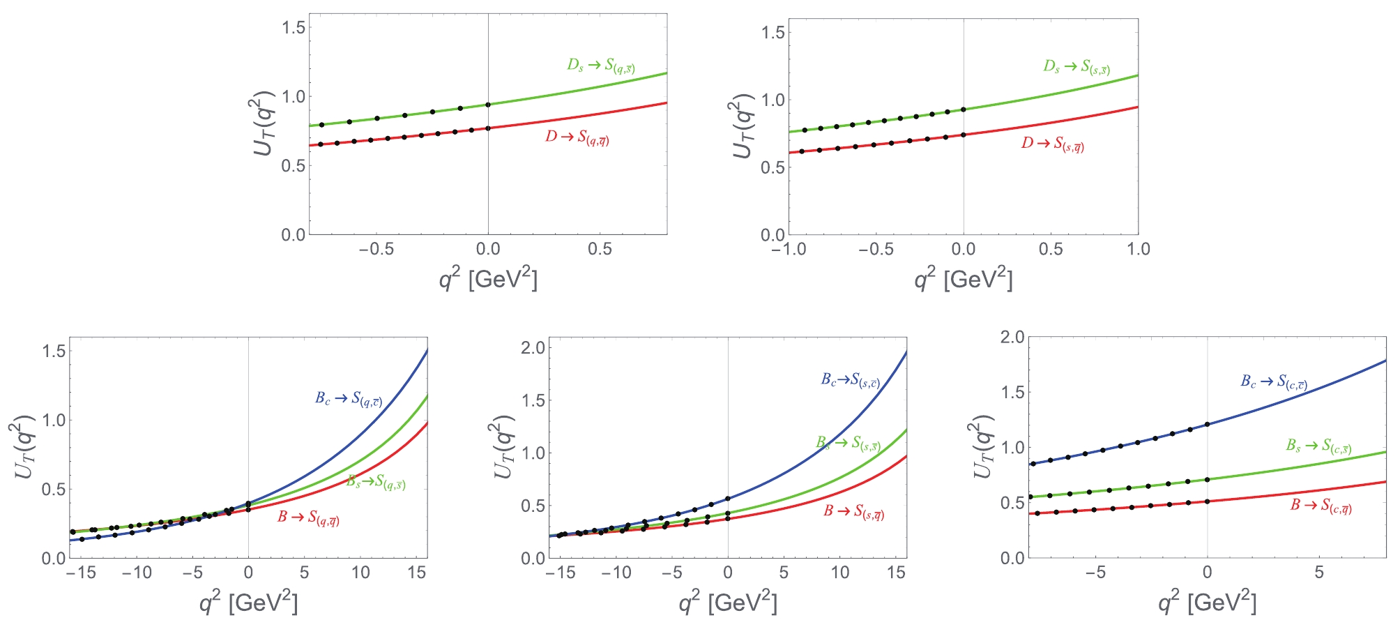
Figure 6. (color online) Same as Fig. 5 except for
$ D_{q,s}\to S $ and$ B_{q,s,c}\to S $ transitions.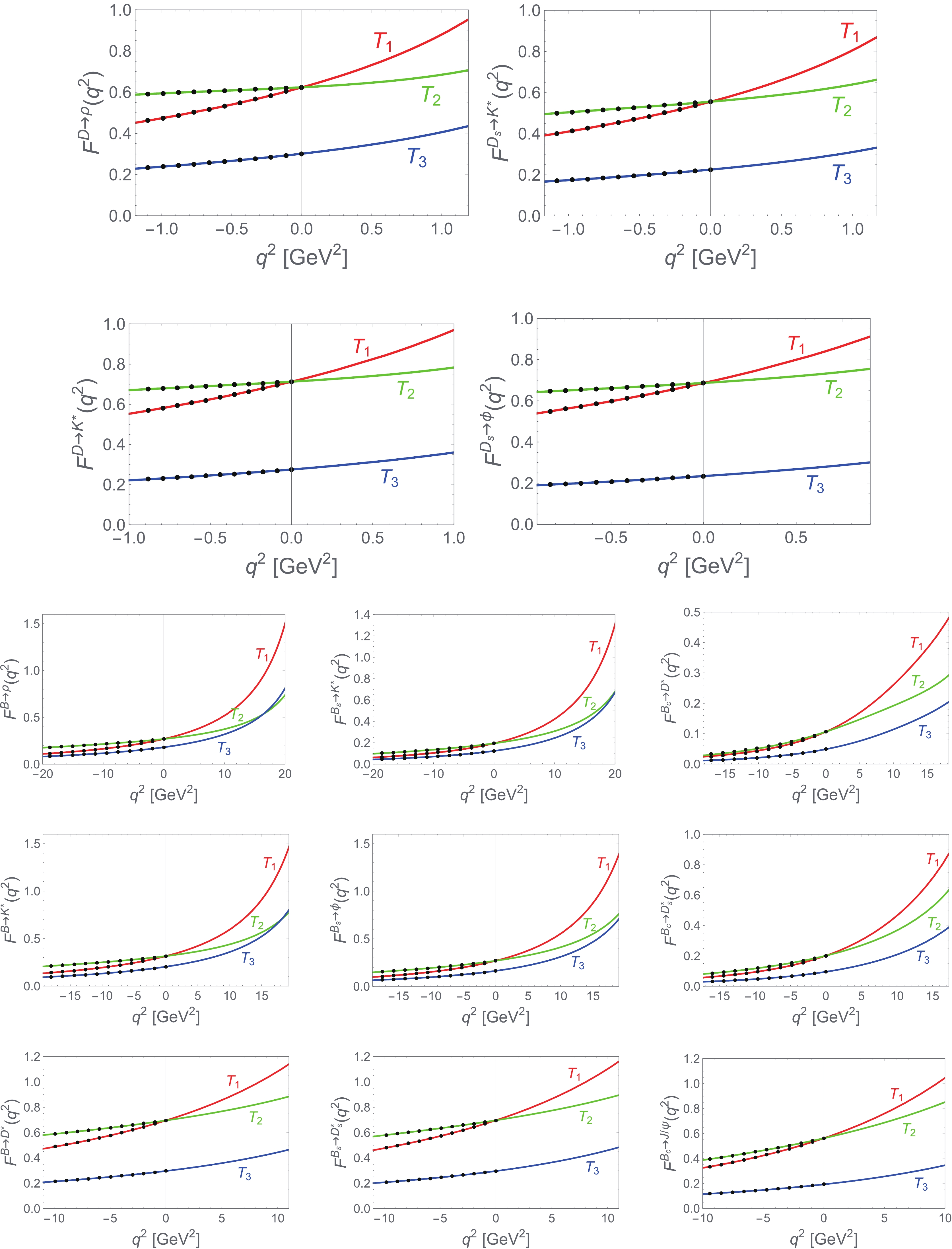
Figure 7. (color online) Same as Fig. 5 except for
$ D_{q,s}\to V $ and$ B_{q,s,c}\to V $ transitions.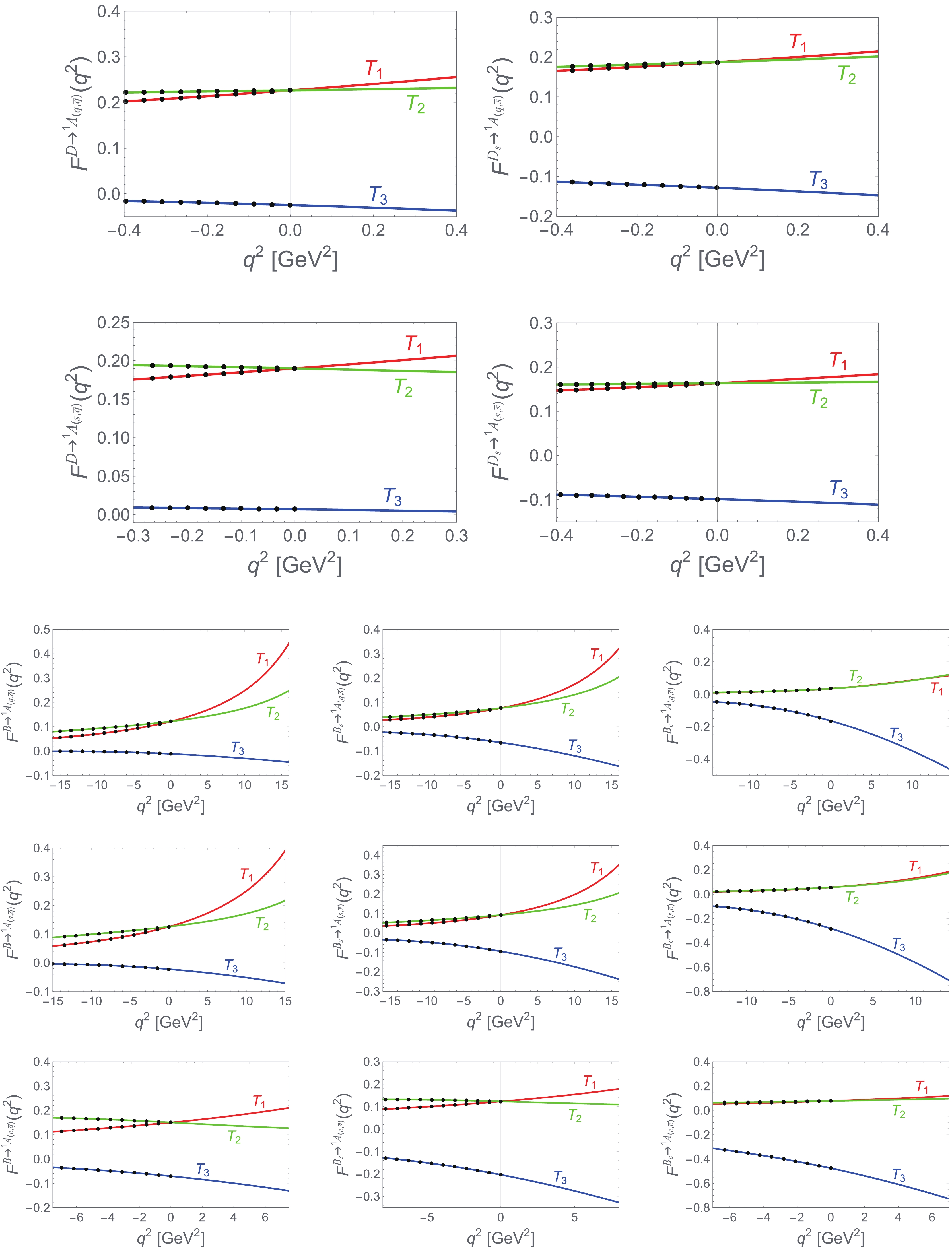
Figure 8. (color online) Same as Fig. 5 except for
$ D_{q,s}\to {^1\!A} $ and$ B_{q,s,c}\to {^1\!A} $ transitions.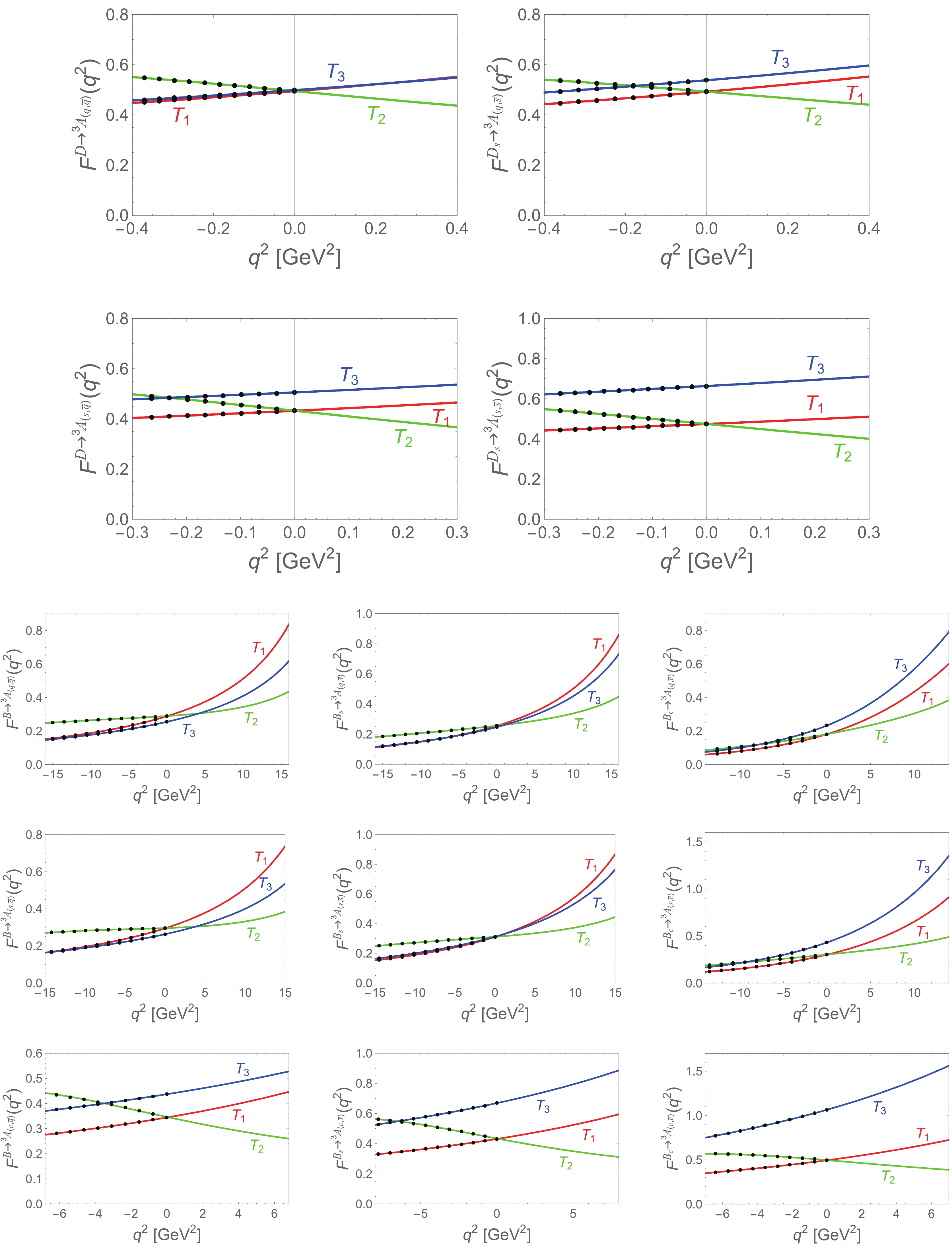
Figure 9. (color online) Same as Fig. 5 except for
$ D_{q,s}\to {^3\!A} $ and$ B_{q,s,c}\to {^3\!A} $ transitions. -
Motivated by the problems of LFQMs, we investigated the tensor matrix elements and relevant form factors of
$ P\to P,\,S,\,V $ , and A transitions within the SLF and the CLF approaches. The self-consistency and Lorentz covariance of the CLF predictions for the tensor matrix elements and form factors are analyzed in detail, and moreover, the zero-mode effects and the relation between valence contribution and SLF result are studied. As pointed out in our previous studies, the covariance is in fact violated in the CLF QM with the traditional correspondence scheme (Type-I) between the manifest covariant BS and the LF approaches; moreover, for$ P\to V $ and A transitions, the tensor form factors extracted via$ \lambda = 0 $ and$ \pm $ polarization states of V and A mesons are inconsistent with each other,$ [{\cal F}]^{\rm {full}}_{\lambda = 0}\neq [{\cal F}]^{\rm {full}}_{\lambda = +}\neq [{\cal F}]^{\rm {full}}_{\lambda = -} $ (Type-I), which implies that CLF QM has a problem of self-consistency. Two such problems have the same origin (the non-vanishing$ \omega $ -dependent spurious contributions associated with B functions), and can be resolved simultaneously by employing the improved Type-II correspondence scheme, which requires an additional replacement$ M\to M_0 $ relative to the traditional Type-I scheme. Within the Type-II scheme, the zero-mode corrections are only responsible for neutralizing spurious$ \omega $ -dependent contributions associated with C functions, but do not contribute numerically to the form factors; and the valence contributions in the CLF QM are exactly the same as the SLF results. The findings mentioned above confirm again the main conclusions obtained in Ref. [84] and our previous studies [85–87].Besides, we find a “novel” self-consistence problem of the CLF approach with the traditional Type-I scheme. Different strategies for dealing with the trace term, S, in the CLF matrix element would result in different formulas for the tensor form factors
$ T_{2(3)} $ of$ P\to V $ and A transitions, and the numerical results are also inconsistent with each other within the Type-I scheme; however, interestingly, this new inconsistency problem can also be overcome numerically by employing the Type-II scheme. Finally, using the CLF approach with the covariant and self-consistent Type-II scheme, the theoretical predictions for the tensor form factors of$ c\to q\,,s $ ($ q = u\,,d $ ) induced$ D_{q,s}\to P,\,S,\,V,\,A $ and$ b\to q\,,s\,,c $ induced$ B_{q,s,c}\to P,\,S,\,V,\,A $ transitions are updated. -
The tensor form factors of
$ P\to V $ transition in the CLF QM have been obtained in previous studies [81, 82], and can also been written as Eq. (53) with the integrands,$\tag{A1} \begin{split} \widetilde{T}_1^{\rm{ CLF}} = &2A_1^{(1)}\left[M'^2-M''^2-2m'^2_1-2\hat N'_1+q^2+2\left(m'_1m_2+m''_1m_2-m'_1m''_1\right)\right]-8A_1^{(2)}+(m'_1+m''_1)^2+\hat N'_1+\hat N''_1-q^2+4\left(M'^2-M''^2\right)\left(A_2^{(2)}-A_3^{(2)}\right)\\ &+4q^2\left(-A_1^{(1)}+A_2^{(1)}+A_3^{(2)}-A_4^{(2)}\right)-\frac{4}{D''_{V,{\rm {con}}}}\left(m'_1+m''_1\right)A_1^{(2)}\,, \end{split} $

$\tag{A2} \begin{split} \widetilde{T}_2^{\rm{ CLF}} = &\widetilde{T}_1^{\rm{ CLF}}+\frac{q^2}{M'^2-M''^2}\bigg\{2A_2^{(1)}\left[M'^2-M''^2-2m'^2_1-2\hat N'_1+q^2+2\left(m'_1m_2+m''_1m_2-m'_1m''_1\right)\right]\\ &-8A_1^{(2)}-2M'^2+2m'^2_1+\left(m'_1+m''_1\right)^2+2(m_2-2m'_1)m_2+3\hat N'_1+\hat N''_1-q^2+2Z_2\\ &+4\left(q^2-2M'^2-2M''^2\right)\left(A_2^{(2)}-A_3^{(2)}\right)-4\left(M'^2-M''^2\right)\left(-A_1^{(1)}+A_2^{(1)}+A_3^{(2)}-A_4^{(2)}\right)-\frac{4}{D''_{V,{\rm {con}}}}\left(m''_1-m'_1+2m_2\right)A_1^{(2)} \bigg\}\,, \end{split} $

$\tag{A3} \begin{split} \widetilde{T}_3^{\rm{ CLF}} = &-2A_2^{(1)}\left[M'^2-M''^2-2m'^2_1-2\hat N'_1+q^2+2\left(m'_1m_2+m''_1m_2-m'_1m''_1\right)\right]+8A_1^{(2)}\\ &+2M'^2-2m'^2_1-(m'_1+m''_1)^2-2(m_2-2m'_1)m_2-3\hat N'_1-\hat N''_1+q^2-2Z_2-4\left(q^2-M'^2-3M''^2\right)\left(A_2^{(2)}-A_3^{(2)}\right)\\ &+\frac{4}{D''_{V,{\rm {con}}}}\bigg\{\left(m''_1-m'_1+2m_2\right)\left[A_1^{(2)}+\left(M'^2-M''^2\right)\left(A_2^{(2)}+A_3^{(2)}-A_1^{(1)}\right)\right]\\ &+\left(m'_1+m''_1\right)\left(M'^2-M''^2\right)\left(A_2^{(1)}-A_3^{(2)}-A_4^{(2)}\right)+m'_1\left(M'^2-M''^2\right)\left(A_1^{(1)}+A_2^{(1)}-1\right) \bigg\}\,. \end{split} $

The results for
$ P\to A $ transition can be obtained via. the relations given by Eqs. (59) and (60). -
The masses of valence quark and Gaussian parameters
$ \beta $ are essential inputs for computing the form factors. For the former, we take [87]$\tag{B1} \begin{split} m_q& = 230\pm40\,{\rm {MeV}}\,,\quad m_s = 430\pm60\,{\rm {MeV}}\,,\\ m_c& = 1600\pm300\,{\rm {MeV}}\,,\quad m_b = 4900\pm400\,{\rm {MeV}}\,, \end{split} $

which can properly cover the fitting results and suggested values given in the previous studies, for instance, the result obtained via variational analyses of meson mass spectra for the Hamiltonian with a smeared-out hyperfine interaction [89], the values obtained by the variational principle for the linear and harmonic oscillator (HO) confining potentials, respectively [90], the fitting results obtained via decay constants and mean square radii of mesons [29], some commonly used values in the LFQMs [60, 61], etc. For the latter, its value for a given meson can be obtained by fitting to the data of decay constant. Using the data of decay constant,
$ f_{P,V} $ , collected in Ref. [85] and the default values of quark masses given by Eq. (94), we obtained the values of$ \beta $ collected in Table B1, where it has been assumed that$ \beta_{q_1\bar{q}_2} $ is universal for$ P(V) $ and$ S(A) $ mesons due to the lack of data for$ f_{S,A} $ . In addition, the self-consistent Type-II scheme is employed for computing decay constants.$ \beta_{q\bar{q}} $ 

$ \beta_{s\bar{q}} $ 

$ \beta_{s\bar{s}} $ 

$ \beta_{c\bar{q}} $ 

$ \beta_{c\bar{s}} $ 

P (S) $ 348\pm1 $ 

$ 365\pm2 $ 

$ 384\pm3 $ 

$ 473\pm12 $ 

$ 543\pm10 $ 

V (A) $ 312\pm6 $ 

$ 313\pm10 $ 

$ 348\pm6 $ 

$ 429\pm13 $ 

$ 530\pm19 $ 

$ \beta_{c\bar{c}} $ 

$ \beta_{b\bar{q}} $ 

$ \beta_{b\bar{s}} $ 

$ \beta_{b\bar{c}} $ 

$ \beta_{b\bar{b}} $ 

P (S) $ 753\pm14 $ 

$ 552\pm10 $ 

$ 606\pm12 $ 

$ 939\pm11 $ 

$ 1394\pm12 $ 

V (A) $ 703\pm7 $ 

$ 516\pm15 $ 

$ 568\pm10 $ 

$ 876\pm20 $ 

$ 1390\pm12 $ 

Table B1. Gaussian parameters
$ \beta $ (in units of MeV).
Tensor form factors of P→ P, S, V and A transitions within standard and covariant light-front approaches
- Received Date: 2020-03-12
- Available Online: 2020-08-01
Abstract: We investigate the tensor form factors of


 DownLoad: