


 Abstract
 HTML
HTML Reference
 Related
 PDF
PDF


-
In the past five years, numerous novel narrow bottom baryons were identified. The latest one was discovered in 2018, when the LHCb Collaboration observed a novel narrow structure with the statistical significance of 9.2
$ \sigma $ in the$ \Lambda_b^{0}K^{-} $ and$ \Xi_b^{0}\pi^{-} $ invariant mass spectra, named$ \Xi_b(6227)^{-} $ [1]. The observed resonance parameters of the structure are$ \begin{split} M =& 6226.9\pm{2.0}({\rm stat})\pm0.3({\rm syst})\pm{}0.2(\Lambda^0_b)\; {\rm{MeV}},\\ \Gamma =& 18.1\pm5.4({\rm stat})\pm1.8({\rm syst})\; {\rm{MeV}}. \end{split} $

(1) The observed channel indicates that the isospin of the
$ \Xi_b(6227)^{-} $ is$ 1/2 $ .However, its spin-parity has not been determined by experiment. Assuming different assignments for its spin-parity, some theoretical interpretations were already discussed in the literature. Considering the
$ \Xi_b(6227) $ as a conventional bottom baryon, the spin-parity was assigned to be$ J^P = 3/2^- $ or$ J^P = 5/2^- $ in Refs. [2-6]. Besides supposing that$ \Xi_b(6227) $ is a conventional bottom baryon, it is also described as a$ S- $ wave dynamically generated resonance with a dominant$ \bar{K}\Sigma_b $ configuration [7, 8]. However, a different conclusion was finally obtained, namely that the$ \Xi_b(6227) $ is a pure$ \bar{K}\Sigma_b $ bound state with$ J^P = 1/2^{-} $ [9].To date, the inner structure of this state remains unclear, and further efforts are necessary. In theory, an investigation of the decay properties may provide more information on the nature of the
$ \Xi_b(6227) $ . Regarding the$ \Xi_b(6227) $ as a conventional bottom baryon, a strong decay width has been computed [2-6]. The results indicate that the$ \Xi_b(6227) $ interpretation as a conventional three quark state is most in agreement with its experimental total width. However, the$ S- $ wave$ \bar{K}\Sigma_b $ assignment for the$ \Xi_b(6227) $ is likewise supported by studying the strong decay widths [7-9]. The two-body allowed strong decay widths from different model are consistent with each other within errors. Hence, based on the analysis of the two-body allowed strong decays, the$ \Xi_b(6227) $ is not only considered as a conventional three quark state, but also as an S-wave$ \bar{K}\Sigma_b $ molecular configuration. Theoretical investigations on other decay modes will be helpful to determine whether the$ \Xi_b(6227) $ is a conventional bottom baryon or a molecular state.Radiative decays may be helpful to distinguish the internal structure of the
$ \Xi_b(6227) $ , as the coupling of the photon to the constituent$ \bar{K} $ meson and$ \Sigma_b $ baryon of the$ \Xi_b(6227) $ is essentially different from that of the quark models, in which the photon couples directly to the quark system [10]. Therefore, a precise measurement of the radiative decays is useful to test different interpretations of the$ \Xi_b(6227) $ . However, to date, no study addressed the radiation decays of the$ \Xi_b(6227) $ . In the present study, we continue our investigation of the$ \Xi_b(6227) $ properties in terms of its radiative decay in the hadronic molecule approach developed in our previous study [9].This paper is organized as follows. The theoretical formalism is explained in Sec. 2. The predicted partial decay widths are presented in Sec. 3, followed by a short summary in the last section.
-
In our previous study [9], the
$ \Xi_b(6227) $ is interpreted as a pure$ \bar{K}\Sigma_b $ bound state with$ J^P = 1/2^{-} $ by studying the strong decay model, where consistency with the observed strong decay width of the$ \Xi_b(6227) $ was achieved in a hadronic molecule interpretation [9]. According to the pure$ \bar{K}\Sigma_b $ molecular scenario, we calculate the radiative decay widths$ \Xi_b(6227)\to\Xi_b\gamma $ and$ \Xi_b(6227)\to\Xi_b^{'}\gamma $ in this study to elucidate the internal structure of the$ \Xi_b(6227) $ . In the$ \bar{K}\Sigma_b $ molecular scenario, the$ \Xi_b(6227) $ must couple to its components via the$ S- $ wave, and the corresponding effective Lagrangian assumes the following form [9, 11]$ \begin{split} {\cal{L}}_{\Xi_b(6227)} =& g_{\Xi_b(6227)\bar{K}\Sigma_b}\Phi[(k_1\omega_{\Sigma_b}-k_2\omega_{\bar{K}})^2]\\ &\times\bar{\Xi}_b(6227)\vec{\tau}\cdot\vec{\Sigma}_b\bar{K} , \end{split} $

(2) where
$ \omega_{ij} = m_i/(m_i+m_{j}) $ , with$ m_i $ as the mass of the baryon or meson.$ k_1 $ and$ k_2 $ denote the four-momenta of the$ \bar{K} $ meson and$ \Sigma_b $ baryon, respectively. From Refs. [9, 11-13], we find that the correlation function$ \Phi(p^2)\doteq \exp(-p_E^2/\Lambda^2) $ is not only introduced to describe the distributions of the$ \bar{K} $ meson and$ \Sigma_b $ baryon in the hadronic molecule, but also plays a role in stopping the Feynman diagrams ultraviolet divergence.$ p_E $ denotes the Euclidean Jacobi momentum, and$ \Lambda $ is the size parameter that characterizes the distribution of components inside a molecule.$ \Lambda $ is a free parameter, and it is usually set to be about 1 GeV to reproduce the experimentally observed decay width in the literature [9, 11-13]. In this study, we vary$ \Lambda $ in a range of 0.9 GeV$ \leqslant\Lambda\leqslant{}1.10 $ GeV.In the above Lagrangian, the remaining unknown coupling constant
$ g_{\Xi_b(6227)\Sigma_b\bar{K}} $ is computed by the compositeness condition [14, 15], which indicates that the renormalization constants of a composite particle wave function should be zero, i.e.,$ Z_{\Xi_b(6227)} = 1-\frac{{\rm d}{\cal{S}}[\Xi_b(6227)]}{{\rm d}k\!\!\!/_0}\bigg|_{k\!\!\!/_0 = m_{\Xi_{b}(6227)}} = 0 , $

(3) where the
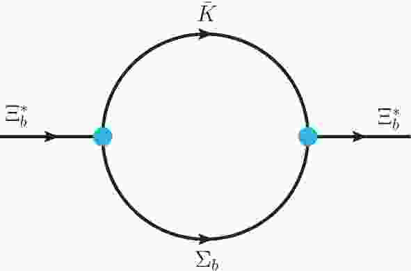
$ {\cal{S}}[\Xi_b(6227)] $ is the mass operator of the$ \Xi_b(6227) $ corresponding to the diagrams in Fig. 1. With the effective Lagrangian in Eq. (2) and the compositeness condition in Eq. (3), we obtain the coupling constant of the$ \Sigma_b\bar{K} $ molecule to its components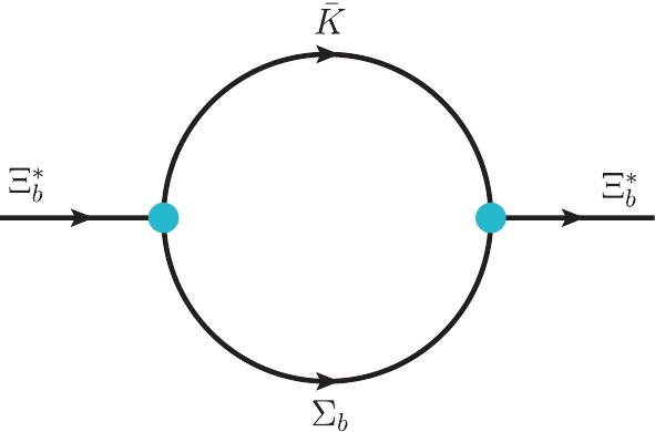
Figure 1. (color online) Self-energy of the
$ \Xi_b^{*}$ state.$ \begin{split} \frac{1}{g^2_{\Xi_b(6227)\Sigma_b\bar{K}}} =& \sum\limits_{i = 1}^{2}{\cal{A}}^2_{i}\int_{0}^{\infty}{\rm d}\alpha\int_{0}^{\infty}{\rm d}\beta\frac{1}{16\pi^2z^2}\\ &\times\left[-\frac{\Delta_i}{2z}-\frac{2}{\Lambda^2}m_{\Xi_b^{*}}\left({\cal{M}}_{i}-\frac{\Delta_im_{\Xi_b^{*}}}{2z}\right){\cal{F}}_i\right]\\ &\times\exp\left\{-\frac{1}{\Lambda^2}\left[{\cal{F}}_im^2_{\Xi_b^{*}}+\alpha{}{\cal{M}}_i^2+\beta{}m_i^2\right]\right\} , \end{split} $

(4) where
$ {\cal{F}}_i = -2\omega_i^2+\frac{\Delta^2_i}{4z}-\beta $ and$ \Delta_i = -4\omega_i-2\beta $ with$ i = 1 $ and 2 denoting the molecule component$ K^{-}\Sigma_b^0 $ and$ \bar{K}^{0}\Sigma_b^{-} $ , respectively.$ {\cal{M}}_i $ and$ m_i $ are the mass of the$ \Sigma_b $ baryon and the mass of the$ \bar{K} $ meson, respectively. The isospin-spin symmetry requiring the coupling of the$ \Xi_b^{-}\Sigma_b^{-}\bar{K}^{0} $ vertex is$ \sqrt{2} $ times lager than the one of the$ \Xi_b^{-}\Sigma_b^{0}K^{-} $ . Employing those ratios and the$ {\cal{A}}_i $ listed$ {\cal{A}}_i = \left\{ {\begin{array}{*{20}{c}} \sqrt{2} & {i = \Sigma_b^{-}\bar{K}^{0}} \\ 1 & {i = \Sigma_b^{0}K^{-}}. \end{array}} \right.$

(5) In the present hadronic molecular scenario, the diagrams contributing to the
$ \Xi_b(6227)^{-}\to\Xi^{-}_b\gamma $ and$ \Xi_b(6227)^{-}\to\Xi_b^{'-}\gamma $ decay are presented in Fig. 2.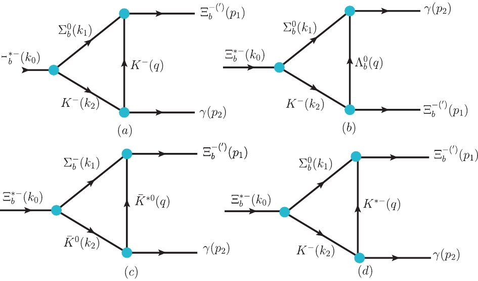
Figure 2. (color online) Feynman diagrams for the
$ \Xi_b(6227)^{-}\to\Xi_b^{-}\gamma$ and$ \Xi_b(6227)^{-}\to\Xi_b^{'-}\gamma$ decay processes. We show the definitions of the kinematics ($ k_0,k_1,k_2,p_1,p_2$ , and q) used in the calculation.To compute the radiative decays of the diagrams shown in Fig. 2, the effective Lagrangian densities related to the photon fields are required, which are [16, 17]
$ \begin{split} {\cal{L}}_{K^{*}K\gamma} =& \frac{g_{K^{*+}K^{+}\gamma}}{4}e\epsilon^{\mu\nu\alpha\beta}F_{\mu\nu}K^{*+}_{\alpha\beta}K^{-}\\ & +\frac{g_{K^{*0}K^{0}\gamma}}{4}e\epsilon^{\mu\nu\alpha\beta}F_{\mu\nu}K^{*0}_{\alpha\beta}\bar{K}^{0}+{\rm h.c.}, \end{split} $

(6) $ {\cal{L}}_{KK\gamma} = {\rm i} eA_{\mu}K^{-} \overleftrightarrow{\partial}^{\mu}K^{+} , $

(7) $ {\cal{L}}_{\gamma{}\Sigma_b\Lambda_b^0} = \frac{e\mu_{\Sigma_b\Lambda_b}}{2m_{\Lambda_b^0}}\bar{\Sigma}_b^0\sigma_{\mu\nu}\partial^{\nu}A^{\mu}\Lambda_b^0+ {\rm h.c.} , $

(8) where the strength tensor is defined as
$ F_{\mu\nu} = \partial_{\mu}A_{\nu}-\partial_{\nu}A_{\mu} $ and$ K^{*}_{\mu\nu} = \partial_{\mu}K^{*}_{\nu}-\partial_{\nu}K^{*}_{\mu} $ . The$ \alpha = e^2/4\pi = 1/137 $ is the electromagnetic fine structure constant. The$ \mu_{\Sigma_b\Lambda_b} = -1.37{}\mu $ is the transition magnetic moment [18], where$ \mu $ is in the units of the nuclear magneton. The coupling constant$ g_{K^{*+}K^{+}\gamma} $ and$ g_{K^{*0}K^{0}\gamma} $ is determined from the partial decay width of$ K^{*+}\to{}K^{+}\gamma $ and$ K^{*0}\to{}K^{0}\gamma $ , which is obtained from Eq. (6),$ \Gamma(K^{*+}\to{}K^{+}\gamma) = \frac{\alpha{}g^2_{K^{*+}K^{+}\gamma}}{24}m_{K^{*+}}(m^2_{K^{*+}}-m^2_{K^{+}}), $

(9) $ \Gamma(K^{*0}\to{}K^{0}\gamma) = \frac{\alpha{}g^2_{K^{*0}K^{0}\gamma}}{24}m_{K^{*0}}(m^2_{K^{*0}}-m^2_{K^{0}}) , $

(10) where
$ m_{K^{*}} $ and$ m_{K} $ are the mass of$ K^{*} $ and kaon, respectively.According to the experimental widths
$ \Gamma(K^{*+}\to{}K^{+}\gamma) = $ 0.0503 keV [19],$ \Gamma(K^{*0}\to{}K^{0}\gamma) = 0.125 $ keV [19], and the masses of the particles shown in Table 1, the coupling constant$ g_{K^{*}K\gamma} $ is fixed as$\Sigma_b^{+}$ 

$\Sigma_b^{0}$ 

$\Sigma_b^{-}$ 

$\Lambda^{0}_b$ 

$\Xi_b^{-}$ 

$\Xi_b^{'-}$ 

$5811.3$ 

$5813.4$ 

$5815.5$ 

$5619.6$ 

$5794.5$ 

$5935.02$ 

$K^{0}$ 

$K^{*0}$ 

$K^{*\pm}$ 

$K^{\pm}$ 

$\pi^{\pm}$ 

$497.611$ 

$898.36$ 

$891.66$ 

$493.68$ 

$139.57$ 

Table 1. Masses of particles in present study (in units of MeV).
$ g_{K^{*+}K^{+}\gamma} = 0.580\; {{\rm{GeV}}^{-1}},\; \; \; \; \; g_{K^{*0}K^{0}\gamma} = -0.904\; {{\rm{GeV}}^{-1}}. $

(11) The signs of these coupling constants are fixed by the quark model.
To evaluate the diagrams in Fig. 2, in addition to the Lagrangian in Eqs. (2), (6), (7), the following effective Lagrangians, responsible for heavy baryons and pseudoscalar mesons interactions, are needed as well [20]
$ \begin{split} {\cal{L}}_{B\phi} =& g_1\langle\bar{B}_6\gamma_{\mu}\gamma_5u^{\mu}B_{6}\rangle+g_2\langle\bar{B}_6\gamma_{\mu}\gamma_5u^{\mu}B_{\bar{3}}+{\rm H.c.} \rangle\\ & +g_6\langle\bar{B}_{\bar{3}}\gamma_{\mu}\gamma_5u^{\mu}B_{\bar{3}}\rangle . \end{split} $

(12) Where the coupling constant
$ g_1 = -\sqrt{\frac{8}{3}}g_2 $ and$ g_6 = 0 $ [20].$ u^{\mu} $ is the axial vector combination of the pseudoscalar-meson fields and its derivatives,$ u^{\mu} = {\rm i}(u^{\dagger}\partial^{\mu}u-u\partial^{\mu}u^{\dagger}), $

(13) where the
$ u^2 = U = \exp({\rm i}\frac{\phi}{f_0}) $ ,$ f_0 $ = 92.4 MeV, and the pseudoscalar-meson octet$ \phi $ is represented by the$ 3\times3 $ matrix$ \phi = \sqrt 2 \left( {\begin{array}{*{20}{c}} {\dfrac{{{\pi ^0}}}{{\sqrt 2 }} + \dfrac{\eta }{{\sqrt 6 }}}&{{\pi ^ + }}&{{K^ + }}\\ {{\pi ^ - }}&{ - \dfrac{{{\pi ^0}}}{{\sqrt 2 }} + \dfrac{\eta }{{\sqrt 6 }}}&{{K^0}}\\ {{K^ - }}&{{{\bar K}^0}}&{ - \dfrac{2}{{\sqrt 6 }}\eta } \end{array}} \right). $

(14) The particle assignment for the
$ J = 1/2 $ bottom baryons of the$ B_{\bar{3}} $ and$ B_{6} $ representations is [20, 21]$ {B_{\bar 3}} = \left( {\begin{array}{*{20}{c}} 0&{\Lambda _b^0}&{\Xi _b^0}\\ { - \Lambda _b^0}&0&{\Xi _b^ - }\\ { - \Xi _b^0}&{ - \Xi _b^ - }&0 \end{array}} \right), $

(15) $ {B_6} = \left( {\begin{array}{*{20}{c}} {\Sigma _b^ + }&{\sqrt {\dfrac{1}{2}} \Sigma _b^0}&{\sqrt {\dfrac{1}{2}} \Xi _b^{0'}}\\ {\sqrt {\dfrac{1}{2}} \Sigma _b^0}&{\Sigma _b^ - }&{\sqrt {\dfrac{1}{2}} \Xi _b^{ - '}}\\ {\sqrt {\dfrac{1}{2}} \Xi _b^{0'}}&{\sqrt {\dfrac{1}{2}} \Xi _b^{ - '}}&{\Omega _b^ - } \end{array}} \right). $

(16) The coupling
$ g_2 $ is fixed from the strong decay width of$ \Sigma_b\to{}\Lambda_b^0\pi $ . Using Eqs. (12)–(16), the two-body decay width$ \Gamma(\Sigma_b\to{}\Lambda_b^0\pi) $ is related to$ g_2 $ as$ \Gamma(\Sigma_b\to{}\Lambda_b^0\pi) = \frac{g_2^2}{\pi{}f_0^2}\frac{(m_{\Sigma_b}+m_{\Lambda_b^0})^2}{(m_{\Sigma_b}+m_{\Lambda_b^0})^2-m^2_{\pi}}{\cal{P}}^3_{\pi{}\Lambda_b^{0}}, $

(17) where the
$ m_{\Sigma_b} $ ,$ m_{\Lambda_b^0} $ , and$ m_{\pi} $ are the masses of the$ \Sigma_b $ baryon,$ \Lambda_b^{0} $ baryon, and$ \pi $ meson, respectively. The$ {\cal{P}}_{\pi{}\Lambda_b^0} $ is the three-momentum of the$ \pi $ in the rest frame of the$ \Sigma_b $ . The Particle Data Group lists the$ \Sigma_b $ predominant decays into$ \Lambda_b^0\pi $ [19], such that its partial width may be approximately equal to the total width of the$ \Sigma_b $ . Using the experimentally determined strong decay width and masses of particles required in the present study, we obtain$ g_2 = 0.252\pm{}0.013 $ .To compute the radiative decay amplitude, the
$ K^{*-}\Sigma^{0}_b\Xi_b^{-(')} $ and$ \bar{K}^{*0}\Sigma^{-}_b\Xi_b^{-(')} $ Lagrangian vertices are required. According to the strategy in Refs. [22, 23], the Lagrangian for the$ K^{*-}\Sigma^{0}_b\Xi_b^{-(')} $ and$ \bar{K}^{*0}\Sigma^{-}_b\Xi_b^{-(')} $ vertices is easily obtained by replacing the charm baryons with the bottom ones, whose procedures are provided in Ref. [9],$ \begin{split} {\cal{L}}_{K^{*}\Sigma_b\Xi_b^{(')}} =& \frac{g}{\sqrt{6}}\bar{\Xi}^{-}_b\gamma^{\mu}\bar{K}_{\mu}^{*0}\Sigma_b^{-}+\frac{g}{2\sqrt{3}}\bar{\Xi}^{-}_b\gamma^{\mu}K_{\mu}^{*-}\Sigma_b^{0}\\ & +\frac{g}{\sqrt{6}}\bar{\Xi}^{0}_b\gamma^{\mu}K^{*-}_{\mu}\Sigma_b^{+}-\frac{g}{2\sqrt{3}}\bar{\Xi}^{0}_b\gamma^{\mu}\bar{K}_{\mu}^{*0}\Sigma_b^{0}\\ &-\frac{g}{\sqrt{2}}\bar{\Xi}^{'0}_b\gamma^{\mu}K^{*-}_{\mu}\Sigma_b^{+}+\frac{g}{2}\bar{\Xi}^{'0}_b\gamma^{\mu}\bar{K}_{\mu}^{*0}\Sigma_b^{0}\\ &+\frac{g}{\sqrt{2}}\bar{\Xi}^{'-}_b\gamma^{\mu}\bar{K}_{\mu}^{*0}\Sigma_b^{-}+\frac{g}{2}\bar{\Xi}^{'-}_b\gamma^{\mu}K_{\mu}^{*-}\Sigma_b^{0}+{\rm h.c.}, \end{split} $

(18) where the coupling constant
$ g = 6.6 $ is obtained from Ref. [23].In the radiative decay of the
$ \Xi_b(6227)^{-}\to\Xi_b^{-}\gamma $ and$ \Xi_b(6227)^{-}\to\Xi_b^{'-}\gamma $ , a photon can be emitted from the kaon meson and$ \Sigma_b $ baryon. The triangle diagrams are listed in Fig. 2, and the corresponding amplitudes are$ \begin{split} {\cal{M}}_{a}& (\Xi_b(6227)^{-}\!\to\!\Xi_b^{-}\gamma) \!=\! -(i)^3\frac{eg_{\Xi_b^{*}\Sigma_b\bar{K}}g_2}{f_0}\!\int\!\frac{{\rm d}^4q}{(2\pi)^4}\Phi[(k_1\omega_{K^{-}}\!-\!k_2\omega_{\Sigma_b^{0}})^2]\bar{u}(p_1)\not\!\!{q}/\gamma_5\frac{k\!\!\!/_1+m_{\Sigma_b^{0}}}{k_1^2-m^2_{\Sigma^{0}_b}}u(k_0) \frac{1}{k_2^2-m^2_{K^{-}}}(k_2^{\mu}+q^{\mu})\frac{1}{q^2-m^2_{K^{-}}}\epsilon^{*}_{\mu}(p_2),\\ {\cal{M}}_{b}& (\Xi_b(6227)^{-}\to\Xi_b^{-}\gamma) = 0,\\ {\cal{M}}_{c}& (\Xi_b(6227)^{-}\to\Xi_b^{-}\gamma) = -(i)^3\frac{geg_{\Xi_b^{*}\Sigma_b\bar{K}}g_{\bar{K}^{*0}\bar{K}^{0}\gamma}}{4\sqrt{3}}\int\frac{{\rm d}^4q}{(2\pi)^4}\Phi[(k_1\omega_{\bar{K}^0}-k_2\omega_{\Sigma_b^{-}})^2]\bar{u}(p_1)\gamma_{\eta}\frac{k\!\!\!/_1+m_{\Sigma_b^{-}}}{k_1^2-m^2_{\Sigma^{-}_b}}\\ &\times{}u(k_0)\frac{1}{k_2^2-m^2_{\bar{K}^{0}}}\epsilon_{\rho\nu\alpha\beta}(p_2^{\rho}g^{\nu\mu}-p_{2}^{\nu}g^{\rho\mu})(q^{\alpha}g^{\beta\sigma}-q^{\beta}g^{\alpha\sigma})\left(-g^{\eta\sigma}+\frac{q^{\eta}q^{\sigma}}{m^2_{\bar{K}^{*0}}}\right)\frac{1}{q^2-m^2_{\bar{K}^{*0}}}\epsilon^{*}_{\mu}(p_2),\\ {\cal{M}}_{d}& (\Xi_b(6227)^{-}\to\Xi_b^{-}\gamma) = -(i)^3\frac{geg_{\Xi_b^{*}\Sigma_b\bar{K}}g_{K^{*-}K^{-}\gamma}}{8\sqrt{3}}\int\frac{{\rm d}^4q}{(2\pi)^4}\Phi[(k_1\omega_{K^{-}}-k_2\omega_{\Sigma_b^{0}})^2]\bar{u}(p_1)\gamma_{\eta}\frac{k\!\!\!/_1+m_{\Sigma_b^{0}}}{k_1^2-m^2_{\Sigma^{0}_b}}\\ &\times{}u(k_0)\frac{1}{k_2^2-m^2_{K^{-}}}\epsilon_{\eta\nu\alpha\beta}(p_2^{\rho}g^{\nu\mu}-p_{2}^{\nu}g^{\mu\rho})(q^{\alpha}g^{\beta\sigma}-q^{\beta}g^{\alpha\sigma})\left(-g^{\eta\sigma}+\frac{q^{\eta}q^{\sigma}}{m^2_{K^{*-}}}\right)\frac{1}{q^2-m^2_{K^{*-}}}\epsilon^{*}_{\mu}(p_2),\\ {\cal{M}}_{a}& (\Xi_b(6227)^{-}\to\Xi_b^{'-}\gamma) = \frac{1}{\sqrt{2}}{\cal{M}}_{a}(\Xi_b^{*-}\to\Xi_b^{-}\gamma)|^{g_2\to-g_1}_{m_{\Xi^{-}_b}\to{}m_{\Xi_b^{'-}}},\\ {\cal{M}}_{b}& (\Xi_b(6227)^{-}\to\Xi_b^{'-}\gamma) = (i)^3\frac{eg_2g_{\Xi_b^{*}\Sigma_b\bar{K}}\mu_{\Sigma_b\Lambda_b}}{4f_0m_{\Lambda_b^0}}\int\frac{{\rm d}^4q}{(2\pi)^4}\Phi[(k_1\omega_{K^{-}}-k_2\omega_{\Sigma_b^{0}})^2]\bar{u}(p_1)k\!\!\!/_2\gamma_5\frac{\not\!\!{q}/+m_{\Lambda_b^0}}{q^2-m^2_{\Lambda_b^0}}\\ &\times(\gamma_{\mu}\not\!\!{p}/_2-\not\!\!{p}/_2\gamma_{\mu})\frac{k\!\!\!/_1+m_{\Sigma_b^0}}{k_1^2-m^2_{\Sigma_b^0}}u(k_0)\frac{1}{k_2^2-m^2_{K^{-}}}\epsilon^{*}_{\mu}(p_2),\\ {\cal{M}}_{c} & (\Xi_b(6227)^{-}\to\Xi_b^{'-}\gamma)= \sqrt{3}{\cal{M}}_{c}(\Xi_b(6227)^{-}\to\Xi_b^{-}\gamma)\big|_{m_{\Xi_b^{-}}\to{}m_{\Xi_b^{'-}}},\\ {\cal{M}}_{d}& (\Xi_b(6227)^{-}\to\Xi_b^{'-}\gamma)= \sqrt{3}{\cal{M}}_{d}(\Xi_b(6227)^{-}\to\Xi_b^{-}\gamma)\big|_{m_{\Xi_b^{-}}\to{}m_{\Xi_b^{'-}}}. \end{split} $

(19) The total amplitude of
$ \Xi_b(6227)^{-}\to\Xi_b^{-(')}\gamma $ is$ {\cal{M}}^{T}_{\Xi_b(6227)^{-}\to\Xi_b^{-(')}\gamma} = {\cal{M}}_a+{\cal{M}}_b+{\cal{M}}_c+{\cal{M}}_d. $

(20) After performing the loop integral, the total contributions of the triangle diagrams to the
$ \Xi_b(6227)^{-}\to\Xi_b^{-(')}\gamma $ can be parameterized as$ \begin{split} {\cal{M}}^{T}_{\Xi_b(6227)^{-}\to\Xi_b^{-(')}\gamma} =& \epsilon^{*}_{\mu}(p_2)\bar{u}(p_1)\\ & \times\left(g_1^{\rm Tri}\gamma^{\mu}+g_2^{\rm Tri}\frac{p_1^{\mu}\not\!\!{p}/_{2}}{p_1\cdot{}p_2}\right)u(k_0). \end{split} $

(21) This amplitude cannot satisfy the gauge invariance of the photon field with only triangle diagrams included. To ensure the gauge invariance of the total amplitudes, the contact diagram in Fig. 3 must be included as well. The effective Lagrangian describing the vertex of
$ \Xi_b^{(')}\gamma\Sigma_b\bar{K} $ could be deduced from the one of the$ \Xi_b^{(')}\Sigma_b\bar{K} $ by the minimal substitution$ \partial^{\mu}\to\partial^{\mu}+{\rm i}e{\cal{A}}^{\mu} $ , which is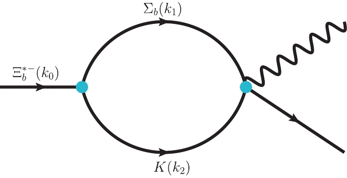
Figure 3. (color online) Contact diagram for
$ \Xi_b(6227)^{-}\to\Xi_b^{-}\gamma$ and$ \Xi_b(6227)^{-}\to\Xi_b^{'-}\gamma$ . We show definitions of the kinematics ($ k_0,k_1,k_2$ , and q) used in the calculation.$ {\cal{L}}_{\Xi_b^{(')}\gamma\Sigma_b\bar{K}} = g_{\Xi_b^{(')}\gamma\Sigma_b\bar{K}}\bar{\Xi}_b^{(')}\gamma_{\mu}\gamma_5{\cal{A}}^{\mu}\bar{K}\Sigma_b. $

(22) By this effective Lagrangian, the amplitude of the contact diagram assumes the form,
$ \begin{split} {\cal{M}}_{\rm Con}& [\Xi_b(6227)^{-}\to\Xi_b^{-(')}\gamma] = g_{\Xi_b^{(')}\gamma\Sigma_b\bar{K}}\int\frac{{\rm d}^4k_1}{(2\pi)^4}\\ & \times\epsilon^{*}_{\mu}(p_2)\Phi[(k_1\omega_{K^{-}}-k_2\omega_{\Sigma_b^{0}})^2]\bar{u}(p_1)\gamma_{\mu}\gamma_5\\ &\times{}\frac{k\!\!\!/_1+m_{\Sigma_b^{0}}}{k_1^2-m^2_{\Sigma^{0}_b}}u(k_0)\frac{1}{k_2^2-m^2_{K^{-}}}. \end{split} $

(23) After performing the loop integral for the above amplitude, we obtain,
$ \begin{split} {\cal{M}}_{\rm Con}& [\Xi_b(6227)^{-}\to\Xi_b^{-(')}\gamma]\\&= \epsilon^{*}_{\mu}(p_2)\bar{u}(p_1)g^{}_{\rm Con}\gamma^{\mu}u(k_0). \end{split} $

(24) The total amplitude of the
$ \Xi_b(6227)^{-}\to\Xi_b^{-(')}\gamma $ is the sum of the triangle diagram and contact term contributions. To maintain an invariant full amplitude gauge, the$g^{}_{\rm Con} = -g_1^{\rm Tri}-g_2^{\rm Tri}$ can be obtained, and the coupling constant$g_1^{\rm Tri}$ and$g_2^{\rm Tri}$ can be evaluated from the amplitudes listed in Eq. (19).Once the amplitudes are determined, the corresponding partial decay widths are obtained, which read,
$ \begin{split} \Gamma(\Xi_b(6227)\to MB) = \frac{1}{2J+1}\frac{1}{8\pi}\frac{|\vec{p}_1|}{m^2_{\Xi_b(6227)}}\overline{|{\cal{M}}|^2}, \end{split} $

(25) where J is the total angular momentum of the
$ \Xi_b(6227) $ state;$ |\vec{p}_1| $ is the three-momenta of the decay products in the center of mass frame; the overline indicates the sum over the polarization vectors of the final hadrons, and MB denotes the decay channel of MB, i.e.,$ \Xi_b\gamma $ and$ \Xi_b^{'}\gamma $ . -
To estimate the radiative decay widths of the considered processes, the relevant coupling constants
$ g_{\Xi_b(6227)\Sigma_b\bar{K}} $ must be discussed first. Regarding the$ \Xi_b(6227) $ as an$ S- $ wave loose$ \Sigma_b\bar{K} $ hadronic molecule, the coupling constant$ g_{\Xi_b(6227)\Sigma_b\bar{K}} $ can be computed by the compositeness condition. As shown in Eq. (4), the coupling constant is dependent on the parameter$ \Lambda $ . With a cutoff$ \Lambda = 0.9-1.1 $ GeV, the corresponding coupling constant varies from 2.68 GeV to 2.47 GeV, as shown in Fig. 4. The coupling constant decreases slowly with the increase in the cut-off, and it is almost independent of$ \Lambda $ . In our previous study [9], the coupling constant was incorrect, being smaller than the one given in this study. However, this does not alter the conclusion that$ \Xi_b(6227) $ only can be considered as$ S- $ wave$ \bar{K}\Sigma_b $ molecule, and the result is shown in Fig. 4.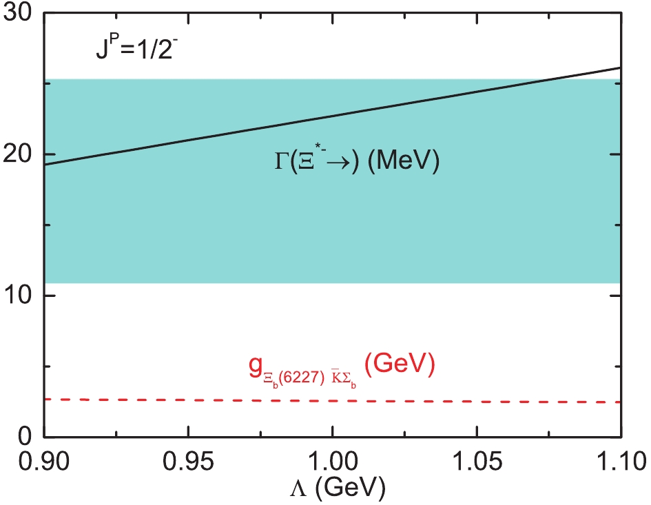
Figure 4. (color online) Coupling constant (red dashed line),
$ g_{\Xi_b(6227)\Sigma_b\bar{K}}$ , and total decay width (black solid line) as a function of the parameter$ \Lambda$ . The cyan band depicts the experimental total width [1].Fig. 5 shows the dependence of the radiative decay widths on the cutoff
$ \Lambda $ . By increasing the cut-off from 0.9 GeV to 1.1 GeV, the radiative decay width of the$ \Xi_b(6227)\to\gamma\Xi^{'}_b $ monotonously increases, albeit very slowly. In particular, the partial width varies from 19.47 to 23.15 keV with the variation of$ \Lambda $ from 0.9 to 1.1 GeV. However, the radiative decay widths decrease for the$ \Xi_b(6227)\to\gamma\Xi_b $ when the cut-off$ \Lambda $ is changed from 0.9 to 1.1 GeV. With the constrained parameter$ \Lambda $ , the partial width of the$ \Xi_b(6227)\to\gamma\Xi_b $ is estimated to be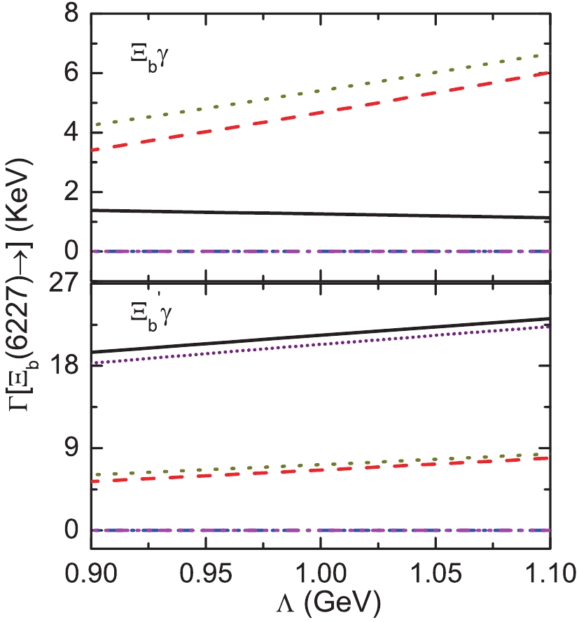
Figure 5. (color online) Total decay width (black solid line) and partial decay widths from
$ {K}^{-}$ (red dash line),$ \bar{K}^{*0}$ (blue dash-dot line),$ \bar{K}^{*-}$ (magenta dash-dot-dot line),$ \Lambda_b^{0}$ (purple short line), and the remainder is the contact term exchange contribution for the$ \Xi_b(6227)$ as a function of the parameter$ \Lambda$ .$ \begin{array}{l} \Gamma(\Xi_b(6227)\to\gamma\Xi_b) = 1.38-1.14\; {\rm{keV}}, \end{array} $

(26) which is weakly dependent on the model parameter. Our calculation indicates that the width of the
$ \Xi_b(6227)\to\gamma\Xi^{'}_b $ is about one order larger than the one of the$ \Xi_b(6227)\to \gamma\Xi_b $ .The contributions to the total width from individual channels are likewise shown in Fig. 5. Because the relative signs of the corresponding amplitude in Fig. 2 are well defined, the analysis of the interference character between various channels is facilitated. The total decay widths obtained are the square of their coherent sum. Regarding the
$ \Xi_b(6227)\to\gamma\Xi_b $ process, the$ K^{-} $ -exchange and contract term provide a dominant contribution to the total decay width, and the amplitude of these two channels are not gauge invariant. The amplitudes corresponding to the$ \Lambda_b^0 $ -exchange and$ \bar{K}^{*} $ -exchange are gauge invariant, and the results indicate that the contributions of these amplitudes are almost three orders of magnitude smaller than those of the amplitudes corresponding to the$ K^{-} $ -exchange and contract term. However, the interferences among them are sizable, which makes the total radiative decay width smaller than the partial decay widths of the$ K^{-} $ -exchange and contact term, respectively. For the transition$ \Xi_b(6227)\to\gamma\Xi^{'}_b $ , the individual contributions of the$ \Lambda_b^0 $ exchange are dominant, almost amounting to the total width. The estimated individual partial decay widths are all insensitive to the$ \Lambda $ . The radiative decay width of the$ \Xi_b(6227) $ into the$ \gamma\Xi_b $ final state is approximately one order of magnitude smaller than into the$ \gamma\Xi^{'}_b $ final state due to the contribution of Fig. 2(b) vanishing in the case of$ \Xi_b(6227)\to\gamma\Xi_b $ .According to Eq. (10) and the experimental width
$ \Gamma(K^{*0}\to{}K^0\gamma) $ = 0.125 keV, the coupling constant$ g_{K^{*0}K^{0}\gamma} $ = 0.904$ {\rm{GeV}}^{-1} $ is fixed. However, it is generally chosen at approximately −0.904$ {\rm{GeV}}^{-1} $ in the literature, and the sign of this coupling constant is fixed by the quark model. If we assume$ g_{K^{*0}K^{0}\gamma} $ = 0.904$ {\rm{GeV}}^{-1} $ , the decay width$ \Gamma_{\gamma{}\Xi_b} $ = 1.39-1.15 keV and$ \Gamma_{\gamma{}\Xi^{'}_b} $ = 19.33-23.08 keV approach the previous results:$ \Gamma_{\gamma{}\Xi_b} $ = 1.38–1.14 keV and$ \Gamma_{\gamma{}\Xi^{'}_b} $ = 19.47–23.15 keV. Hence, our numerical results show that the value of the decay width$ \Gamma_{\gamma{}\Xi_b} $ and$ \Gamma_{\gamma{}\Xi^{'}_b} $ is not sensitive to the negative sign when varying the model parameter$ \Lambda $ from 0.9 to 1.1. -
Presently, there is not sufficient experimental information to determine the spin-parity of the
$ \Xi_b(6227) $ state. The experimental study of its decay behaviors could provide further insigth into its inner structure. However, the strong decay channels are difficult to determine, irrespective whether the$ \Xi_b(6227) $ is a conventional bottom baryon [2-6] or a molecular state [7-9].In the present study, we estimated the partial widths for the radiative decay from the
$ \Xi_b(6227) $ to the$ \Xi^{'}_b $ and$ \Xi_b $ state in a molecular scenario, in which the$ \Xi_b(6227) $ is considered a$ \Sigma_b{}\bar{K} $ hadronic molecule. In the relevant parameter region, the partial widths are evaluated as$ \begin{split} \Gamma(\Xi_b(6227)\to\gamma\Xi_b) =& 1.38-1.14\; {\rm{keV}},\\ \Gamma(\Xi_b(6227)\to\gamma\Xi^{'}_b) = &19.47-23.15\; {\rm{keV}}. \end{split} $

(27) Our estimations indicate that the partial widths for the
$ \Xi_b(6227)\to\gamma\Xi_b $ transition are approximately one order of magnitude smaller than those of$ \Xi_b(6227)\to\gamma\Xi^{'}_b $ .Based on the current integrated luminosity and our estimations, facilities such as the LHCb might be able to detect radiative decays of the
$ \Xi_b(6227) $ baryon in the keV regime. This research can also be performed in the forthcoming Belle II experiment. The study of the radiative decay of the$ \Xi_b(6227) $ baryon employing the quark model is strongly recommended. In comparison with the predicted widths of the quark model, the results in the present study provide further information for the experimental search for the$ \Xi_b(6227) $ baryon. Furthermore, the experimental measurements for these radiative decay processes can be a crucial test for the molecule interpretation of the$ \Xi_b(6227) $ baryon.
Radiative decay of Ξb(6227) in a hadronic molecule picture
- Received Date: 2020-01-03
- Accepted Date: 2020-03-31
- Available Online: 2020-08-01
Abstract: The baryon


 DownLoad: