


 Abstract
 HTML
HTML Reference
 Related
 PDF
PDF


-
The studies of semileptonic decays of
B/Bs meson play an essential role in testing the Standard Model (SM) as well as in the search for new physics (NP) beyond SM, since the lepton flavor universality (LFU) can be examined in this kind of decay modes. LFU implies that all electroweak gauge bosons (Z0 ,γ andW± ) have equivalent couplings to the three generations of leptons, and the only difference arises from the mass differences:me<mμ≪mτ . Therefore, if the experiments were to find signals of lepton flavor violation (LFV), that would be a true challenge for SM.The first observation of the
R(D) andR(D∗) anomalies in semileptonic decaysB→D(∗)lνl withl−= (e−,μ−,τ−) by the BaBar collaboration in 2012 [1, 2] invoked intensive studies of theB→D(∗)lνl decays in the SM framework [3–10] and various NP models [11–18]. With the measurements reported by the Belle and LHCb collaborations [19–25], however, the deviations between the measuredR(D) andR(D∗) and the SM predictions become smaller [26–29]:(1) The latest Belle measurements [24] exhibit an excellent consistency with the averaged SM predictions [3–5, 29]:R(D)={0.307±0.037(stat.)±0.016(syst.),Belle[24]0.299±0.003,SM[29],
(1) R(D∗)={0.283±0.018(stat.)±0.014(syst.),Belle[24]0.258±0.005,SM[29],
(2) since they are compatible within one standard deviation [24, 29].
(2) The combined analysis of currently available measurements ofR(D) andR(D∗) , including the new Belle results [24], gives the following world averaged values:R(D)Exp=0.340±0.027±0.013,R(D∗)Exp=0.295±0.011±0.008,
(3) so that the discrepancy decreases from the previous
3.8σ to3.1σ with respect to the SM expectations [26, 27, 29].(3) Besides the ratiosR(D(∗)) , other physical observables, such as the longitudinal polarization of the tau leptonPτ(D∗) and the fraction of theD∗ longitudinal polarizationFL(D∗) , were measured recently by the Belle collaboration [20, 21, 30]:Pτ(D∗)=−0.38±0.51(stat.)+0.21−0.16(syst.)[20,21],
(4) FL(D∗)=0.60±0.08(stat.)±0.04(syst.)[30].
(5) They are compatible with the SM predictions
Pτ(D∗)= −0.497±0.013 [31],FL(D∗)=0.441(6) [32] and0.457(10) [33] for theB→D∗τˉντ decays.It is clear from the above points that although the anomalies of
R(D(∗)) have become less serious recently, there is still a sizeable discrepancy with respect to the SM expectations, and that they should be investigated with complementary and more precise measurements in order to draw a conclusion. In addition to theB→D(∗)lνl decays, theBs→D(∗)slνl decay mode is one of the best choices for cross examination. Systematic theoretical studies and experimental measurements of the semileptonic decays ofBs meson are therefore very important and should be performed promptly.As illustrated by the Feynman diagrams in Fig. 1, the
Bs→D(∗)sl+νl decays are closely related to theB→D(∗)l+νl decays via the SU(3) flavor symmetry. They are all controlled by the sameb→clν transitions at the quark level, but with a different spectator quark:(u,d) or s quark. As a consequence, in the limit of the SU(3) flavor symmetry, these two sets of semileptonic decays must have very similar properties. If the current anomalies inB→D(∗)lνl decays are indeed induced by contributions from NP, they must appear in theBs→D(∗)slνl decays. It is therefore necessary and very interesting to study theBs→D(∗)slνl decays and to measure the corresponding ratiosR(D(∗)s) and other relevant physical observables, such asPτ(D(∗)s) ,FL(D∗s) andAFB(τ) , in order to check if similar deviations exist.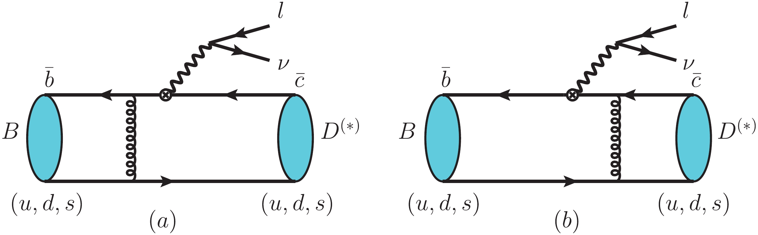
Figure 1. (color online) Leading order Feynman diagrams for the semileptonic decays
B(s)→D(s)l+νl withl=(e,μ,τ) in the PQCD approach.As is well known, the central issue for calculating such semileptonic decays in the SM framework is the estimate of the values and shapes of the form factors
(F+,0(q2),V(q2),A0,1,2(q2)) for theB(s)→D(∗)(s) transitions. However, calculations of these form factors are not easy and they cannot be estimated reliably in the whole range of momentaq2 carried by the lepton pair using a single method, and their extrapolation is indispensable. There are many traditional methods and approaches to estimate the form factors and provide predictions of the ratiosRD(∗) , for example, the heavy quark effective theory (HQET) [4, 5], light cone sum rules (LCSR) [34–36], lattice QCD (LQCD) [37–41] and the perturbative QCD factorization approach (PQCD) [9, 10].In recent years, the PQCD factorization approach has been used to study various kinds of semileptonic decays of
B/Bs/Bc mesons, as given for example in Refs. [9, 10, 42–48]. However, like in many other theoretical approaches, the form factors evaluated using the PQCD approach are only reliable in the lowq2 region. Therefore, extrapolations must be done in order to cover the whole range ofq2 values of the form factorsfi(q2) . In order to improve the reliability of the values and shapes of the six form factors obtained in the PQCD approach, we include the lattice QCD result at the end pointq2max so that the extrapolation from the lowq2 region to the highq2 region is more reliable.In Refs. [9, 10], the
B→D(∗)lνl decays were studied by employing the PQCD approach only [9], or with the inclusion of the lattice QCD input [10]. In Ref. [42], theˉB0s→D(∗)sl−ˉνl decays were studied by employing the PQCD approach without the lattice QCD input. In this paper, we study the semileptonic decays of B andBs mesons simultaneously and focus on the following three tasks:(1) For theBs→D(∗)s andB→D(∗) transitions, we evaluate the relevant form factors in the region0⩽ using the PQCD factorization approach, and then include the lattice QCD result at the end pointq^2_{\max} in the fitting process and extrapolate the form factors in the entire momentum region by employing the Bourrely-Caprini-Lellouch (BCL) parametrization [49, 50] instead of the pole models used in Refs. [9, 10, 42].(2) In addition to the calculations of the branching ratios and the ratiosR(D_s^{(*)}) andR(D^{(*)}) , we also calculate three physical observables (which were not considered in [9, 10, 42]) for the decays of B andB_s mesons: the longitudinal polarization of the tau leptonP_\tau(D_{(s)}^{(*)}) , the fraction ofD_{(s)}^* longitudinal polarizationF_L(D_{(s)}^*) , and the forward-backward asymmetry of the tau leptonA_{FB}(\tau) in the ordinary PQCD approach and the “PQCD +Lattice” approach (i.e. the PQCD approach with the inclusion of the lattice QCD input for the form factors).(3) We present our theoretical predictions, compare them with the available experimental measurements, or the theoretical predictions obtained using other different theories or models.The paper is organized as follows: In Sec. 2, we briefly review the kinematics of the
B^0_s \to D_s^{(*)} l^+ \nu_l decays. The calculations of the form factors for theB^0_s \to D_s^{(*)} transitions are then given. We use the lattice QCD result atq^2_{\max} given by the HPQCD group [41] as input in our extrapolation. Explicit expressions for the differential decay rates and additional physical observables are also given in Sec. 2. In Sec. 3, we present the theoretical predictions of the other physical observables obtained using the PQCD approach, the “PQCD+Lattice” approach and some other models. A short summary is given in the final section. -
In the PQCD approach, the tree-level Feynman diagrams for
B_{(s)} \to D^{(*)}_{(s)} l \nu decays① are shown in Fig. 1. We define theB_{(s)} meson momentum asp_1 , theD_{(s)}/D^*_{(s)} meson momentum asp_2 , and the polarization vectors\epsilon_{L,T} in theD_{(s)}^* atB_{(s)} rest frames as in Ref. [51].\begin{split} p_1& =\frac{m_{B_{(s)}}}{\sqrt{2}}(1,1,0_\bot),\quad p_2 = \frac{r \cdot m_{B_{(s)}}}{\sqrt{2}} (\eta^+,\eta^-,0_\bot), \\ \epsilon_L& = \frac{1}{\sqrt{2}}(\eta^+,-\eta^-,0_\bot), \quad \epsilon_T = (0,0,1), \end{split}
(6) while
\epsilon_L and\epsilon_T denote the longitudinal and transverse polarization of(D^*, D_s^*) mesons, respectively. The parameter\eta^{\pm} and r are defined as:\eta^{\pm} = \eta \pm \sqrt{\eta^2-1},\quad \eta = \frac{1}{2r}\left(1+r^2-\frac{q^2}{m_{B_{(s)}}^2}\right),\quad r = \frac{m_{D_{(s)}^{(*)}}}{m_{B_{(s)}}},
(7) where
q = p_1 - p_2 is the momentum of the lepton pair. The momenta of the spectator quarks inB_{(s)} andD_{(s)}^{(*)} mesons are parametrized ask_1 = \frac{m_{B_{(s)}}}{\sqrt{2}}(0,x_1,k_{1\bot}),\quad k_2 = \frac{r\cdot m_{B_{(s)}}}{\sqrt{2}}(x_2\eta^+,x_2\eta^-,k_{2\bot}),
(8) where
x_1 andx_2 are the fraction of the momentum carried by the light spectator quark in the initialB/B_s meson and the final state mesonD^{(*)}/D_s^{(*)} , respectively.For the
B/B_s meson wave functions, we use the functions from Refs. [51, 52].\Phi_{B_{(s)}}(x,b) = \frac{\rm i}{\sqrt{2N_{\rm c}}} (\not\!\! p_{B_{(s)}} +m_{B_{(s)}}) \gamma_5 \phi_{B_{(s)}} (x,b),
(9) \phi_{B_{(s)}}(x,b)= N_{B_{(s)}} \cdot x^2(1-x)^2 \cdot \exp \bigg[-\frac{x^2 \cdot M_{B_{(s)}}^2}{2 \omega_{B_{(s)}}^2} -\frac{1}{2} (\omega_{B_{(s)}} \cdot b)^2\bigg].
(10) The normalization factor
N_{B_{(s)}} depends on the values of the parameter\omega_{B_{(s)}} and decay constantf_{B_{(s)}} through the normalization relation:\int_0^1{\rm d}x\ \phi_{B_{(s)}}(x,b = 0) = f_{B_{(s)}}/(2\sqrt{6}) . In order to estimate the uncertainties of theoretical predictions, we set the shape parameter\omega_B = 0.40 \pm 0.04 GeV and\omega_{B_s} = 0.50 \pm 0.05 GeV.For
D_{(s)} andD_{(s)}^* mesons, we use the same wave functions as in Ref. [53]\Phi_{D_{(s)}}(p,x) = \frac{\rm i}{\sqrt{6}}\gamma_5 (\not\!\! p_{D_{(s)}}+ m_{D_{(s)}})\phi_{D_{(s)}}(x),
(11) \begin{split} \Phi_{D^*_{(s)}}(p,x) =& \frac{- \rm i}{\sqrt{6}} \left [ {\not\!\! {\epsilon}}_{\rm L}(\not\!\! p_{D^*_{(s)}} +m_{D^*_{(s)}})\phi^{\rm L}_{D^*_{(s)}}(x)\right. \\&\left.+ {\not\!\! {\epsilon}}_{\rm T}(\not \!\!p_{D^*_{(s)}} + m_{D^*_{(s)}})\phi^{\rm T}_{D^*_{(s)}}(x)\right], \end{split}
(12) with the distribution amplitudes
\begin{split} \phi_{ D^{(*)}_{(s)} }(x) =& \frac{ f_{D^{(*)}_{(s)} }}{2\sqrt{6}} \cdot 6x(1-x) \left[ 1+C_{D^{(*)}_{(s)} }(1-2x)\right] \\&\times\exp \bigg[-\frac{\omega^2 b^2 }{2}\bigg], \end{split}
(13) where we set the parameters
C_D = C_{D^*} = C_{D_s} = C_{D_s^*} = 0.5 and\omega = 0.1 . From the heavy quark limit, we assume thatf^{L}_{D^*} = f^{T}_{D^*} = f_{D^*}, \quad f^{L}_{D_S^*} = f^{T}_{D_S^*} = f_{D_s^*},
(14) \phi^{L}_{D^*} =\phi^{T}_{D^*} = \phi_{D^*}, \quad \phi^{L}_{D_s^*} = \phi^{T}_{D_s^*} = \phi_{D_s^*}.
(15) -
The form factors of the
B_{(s)} \to D_{(s)} transition are defined in the same form as in Ref. [54]\begin{split}& \langle D_{(s)}(p_2)|\bar{c}(0)\gamma_{\mu}b(0)|B_{(s)}(p_1)\rangle \!=\! \left[(p_1\!+\!p_2)_{\mu}-\frac{m_{B_{(s)}}^2\!-\!m_{D_{(s)}}^2}{q^2}q_{\mu}\right] \\ & \times F_+(q^2)+ \left[ \frac{m_{B_{(s)}}^2-m_{D_{(s)}}^2}{q^2}q_{\mu} \right] F_0(q^2).\\[-20pt] \end{split}
(16) In order to cancel the poles at
q^2 = 0 ,F_+(0) should be equal toF_0(0) . For convenience, we also define the auxiliary form factorsf_1(q^2) andf_2(q^2) ,\langle D_{(s)}(p_2)|\bar{c}(0)\gamma_{\mu}b(0)|B_{(s)}(p_1)\rangle = f_1(q^2)p_{1\mu}+f_2(q^2)p_{2\mu},
(17) which are related to
F_+(q^2) andF_0(q^2) by the following relations,F_+(q^2) =\frac12\left[f_1(q^2)+f_2(q^2)\right],
(18) \begin{split} F_0(q^2) = &\frac12 f_1(q^2)\left[1+\frac{q^2}{m_{B_{(s)}}^2-m_{D_{(s)}}^2}\right]\\& +\frac12 f_2(q^2)\left[1-\frac{q^2}{m_{B_{(s)}}^2-m_{D_{(s)}}^2}\right]. \end{split}
(19) For vector meson
D^*_{(s)} in the final state, the form factors forB_{(s)} \to D^*_{(s)} transitions areV(q^2) andA_{0,1,2}(q^2) , which are given in the following form [54] :\begin{split} \langle D^*_{(s)}(p_2)|\bar{c}(0) \gamma_{\mu} b(0)|B_{(s)}(p_1)\rangle = \frac{2 i V(q^2)}{m_{B_{(s)}}+m_{D_{(s)}^*}}\epsilon_{\mu \nu \alpha \beta} \epsilon^{* \nu}p_1^\alpha p_2^\beta, \end{split}
(20) \begin{split} \langle D^*_{(s)}(p_2)|\bar{c}(0) \gamma_{\mu}\gamma_5 b(0)|B_{(s)}(p_1)\rangle =& 2 m_{D_{(s)}^*}A_0(q^2)\frac{\epsilon^*\cdot q}{q^2}q_\mu + (m_{B_{(s)}} + m_{D_{(s)}^*})A_1(q^2) \left (\epsilon^*_\mu - \frac{\epsilon^*\cdot q}{q^2}q_\mu \right) \\ & - A_2(q^2)\frac{\epsilon^*\cdot q}{m_{B_{(s)}} + m_{D_{(s)}^*}} \left [(p_1+p_2)_\mu - \frac{m_{B_{(s)}}^2-m_{D_{(s)}^*}^2}{q^2}q_\mu \right ]. \end{split}
(21) The analytical expressions for the form factors mentioned above are the following:
\begin{split} f_1(q^2) =& 8\pi m^2_{B_{(s)}} C_F\int {\rm d}x_1 {\rm d}x_2\int b_1 {\rm d} b_1 b_2 {\rm d} b_2 \phi_{B_{(s)}}(x_1,b_1) \phi_{D_{(s)}}(x_2,b_2) \Bigg\{ \left[ 2 r\left(1-rx_2\right) \right]\cdot H_1(t_1) \\ &+ \left[ 2 r(2 r_c-r) + x_1 r \left (-2+2 \eta+\sqrt{\eta^2-1}-\frac{2\eta}{\sqrt{\eta^2-1}}+\frac{\eta^2}{\sqrt{\eta^2-1}} \right) \right] \cdot H_2(t_2) \Bigg \}, \end{split}
(22) \begin{split}f_2(q^2)& = 8\pi m^2_{B_{(s)}} C_F\int {\rm d}x_1 {\rm d}x_2\int b_1 {\rm d} b_1 b_2 {\rm d} b_2 \phi_{B_{(s)}}(x_1,b_1)\phi_{D_{(s)}}(x_2,b_2) \\ &\times \Bigg\{ \left[ 2-4 x_2 r(1-\eta) \right] \cdot H_1(t_1) + \left[ 4r-2r_c-x_1+\frac{x_1}{\sqrt{\eta^2-1}}(2-\eta) \right] \cdot H_2(t_2) \Bigg \}, \end{split}
(23) where the mass ratios are
r_c = m_c/m_{B_{(s)}} ,r = m_{D_{(s)}}/m_{B_{(s)}} .\begin{split} V(q^2) = 8\pi m^2_{B_{(s)}} C_F\int {\rm d} x_1 {\rm d} x_2\int b_1 {\rm d} b_1 b_2 {\rm d} b_2 \phi_{B_{(s)}}(x_1,b_1)\phi^T_{D^*_{(s)}}(x_2,b_2) \cdot (1+r) \Bigg \{\left[1-rx_2\right] \cdot H_1(t_1) + \left[r+\frac{x_1}{2\sqrt{\eta^2-1}}\right] \cdot H_2(t_2) \Bigg \}, \end{split}
(24) \begin{split} A_0(q^2) =& 8\pi m^2_{B_{(s)}} C_F\int {\rm d}x_1 {\rm d}x_2\int b_1 {\rm d}b_1 b_2 {\rm d} b_2 \phi_{B_{(s)}} (x_1,b_1)\phi^L_{D^*_{(s)}}(x_2,b_2) \Bigg \{ \left[ 1+r -rx_2(2+r-2\eta)\right]\cdot H_1(t_1) \\ &+ \left [r^2+r_c+\frac{x_1}{2}+\frac{\eta x_1}{2\sqrt{\eta^2-1}}\right. \left.+\frac{rx_1}{2\sqrt{\eta^2-1}}\left(1-2\eta\left(\eta+\sqrt{\eta^2-1}\right)\right)\right ]\cdot H_2(t_2) \Bigg \}, \end{split}
(25) \begin{split} A_1(q^2) =& 8\pi m^2_{B_{(s)}} C_F\int {\rm d}x_1 {\rm d}x_2\int b_1 {\rm d}b_1 b_2 {\rm d} b_2 \phi_{B_{(s)}}(x_1,b_1)\phi^T_{D^*_{(s)}}(x_2,b_2)\cdot \frac{r}{1+r} \\ &\times \Bigl \{2 [ 1+\eta-2 r x_2+r\eta x_2 ]\cdot H_1(t_1) + \left[2r_c+2 \eta r-x_1\right]\cdot H_2(t_2) \Bigr \}, \end{split}
(26) \begin{split} A_2(q^2) =& \frac{(1+r)^2(\eta-r)}{2r(\eta^2-1) }\cdot A_1(q^2) - 8\pi m^2_{B_{(s)}} C_F\int {\rm d}x_1 {\rm d}x_2\int b_1 {\rm d} b_1 b_2 {\rm d} b_2\phi_{B_{(s)}} (x_1,b_1) \cdot \phi^L_{D^*_{(s)}}(x_2,b_2) \cdot \frac{1+r}{\eta^2-1}\\& \times \Bigg \{ \left[(1+\eta)(1-r) -rx_2(1-2r+\eta(2+r-2\eta))\right] \cdot H_1(t_1) \\& + \left[ r+r_c(\eta-r)-\eta r^2+r x_1\eta^2-\frac{x_1}{2}(\eta+r)+x_1 \left(\eta r -\frac{1}{2}\right)\sqrt{\eta^2-1}\right] \cdot H_2(t_2) \Bigg \}, \end{split}
(27) where the color factor is
C_F = 4/3 , the mass ratios arer_c = m_c/m_{B_{(s)}} ,r = m_{D^*_{(s)}}/m_{B_{(s)}} and the functionsH_i(t_i) are in the following formH_i(t_i) = h_i(x_1,x_2,b_1,b_2) \cdot \alpha_s(t_i) \exp\left [-S_{ab}(t_i) \right ], \; {\rm for} \; i = (1,2).
(28) The explicit expressions for the hard functions
h_i(x_1,x_2,b_1,b_2) , hard scalest_i and the Sudakov factors[-S_{ab}(t_i)] are given in the Appendix. -
The lattice QCD has advantages in calculating the form factors for large
q^2 , and it is generally believed that the lattice QCD predictions close to or atq^2_{\max} are reliable. In this work, we make use of the lattice QCD predictions of all relevant form factors at the endpointq^2_{\max} as the additional input in the fitting process, so as to make the extrapolation of these form factors from the lowq^2 region toq^2_{\max} more reliable.The form factors used in the lattice QCD are parametrized as follows [55, 56]:
\begin{split} \langle D_{(s)}|\bar{c} V^{\mu} b|B_{(s)}\rangle = & \sqrt{m_{B_{(s)}} m_{D_{(s)}}} \left[ h_+(w)(\upsilon+\upsilon')^{\mu}+h_-(w)(\upsilon-\upsilon')^{\mu} \right], \\ \langle D^*_{(s)}|\bar{c} V^{\mu} b|B_{(s)}\rangle = & \sqrt{m_{B_{(s)}} m_{D^*_{(s)}}} i\varepsilon^{\mu\nu}_{\; \; \; \rho\sigma} \epsilon^*_\nu \upsilon^\rho \upsilon'^\sigma h_V(w), \\ \langle D^*_{(s)}|\bar{c} A^{\mu} b|B_{(s)}\rangle = & \sqrt{m_{B_{(s)}} m_{D^*_{(s)}}} \epsilon^*_\nu \left[ g^{\mu\nu}(1+w)h_{A_1}(w)\right.\\&\left.-\upsilon^\nu(\upsilon^\mu h_{A_2}(w)+\upsilon'^\mu h_{A_3}(w))\right], \\[-12pt] \end{split}
(29) where
\upsilon = p_{B_{(s)}}/m_{B_{(s)}}, \upsilon' = p_{D^{(*)}_{(s)}}/m_{D^{(*)}_{(s)}} , the velocity transfer isw = \upsilon \cdot \upsilon' , and\epsilon is the polarization vector of theD^*_{(s)} meson. With a simple transformation, we can relate them to the form factors used in our work:\begin{split} F_+(q^2)& = \frac{1}{2\sqrt{r}} \left [ (1+r) h_+(w) - (1-r)h_-(w) \right], \\ F_0(q^2) & = \sqrt{r} \left [ \frac{1+w}{1+r}h_+(w) -\frac{w-1}{1-r} h_-(w) \right], \end{split}
(30) where
w = (m^2_{B_{(s)}}+m^2_{D_{(s)}} -q^2)/(2 m_{B_{(s)}} m_{D_{(s)}}) , and\begin{align} V(q^2)& = \frac{1+r}{2\sqrt{r}}h_V(w), \\ A_0(q^2)& = \frac{1}{2\sqrt{r}}\left [ (1+w)h_{A_1}(w)-(1-w r) h_{A_2}(w)+(r-w)h_{A_3}(w) \right ], \\ A_1(q^2)& = \frac{\sqrt{r}}{1+r}(1+w)h_{A_1}(w), \\ A_2(q^2)& = \frac{1+r}{2\sqrt{r}}(r h_{A_2}(w)+h_{A_3}(w)), \end{align}
(31) where
w = (m^2_{B_{(s)}}+m^2_{D^*_{(s)}} -q^2)/(2 m_{B_{(s)}} m_{D^*_{(s)}}) .At the end point
q^2 = q^2_{\max} , we have\begin{split} h_V(1)& = h_{A_1}(1) = h_{A_3}(1), \quad h_{A_2}(1) = 0, \quad h_{A_1}(1) = {\cal {F}}(1), \\ w& = 1, \quad \left [ h_+(1) - \frac{(1-r)}{(1+r)}h_-(1) \right] = {\cal {G}}(1). \\[-15pt] \end{split}
(32) Therefore, the relevant form factors at the endpoint
q^2_{\max} become:\begin{align} F_+(q^2_{\max}) & = \frac{1+r}{2\sqrt{r}} {\cal {G}}(1), \\ V(q^2_{\max})& = A_0(q^2_{\max}) = A_2(q^2_{\max}) = \frac{1}{A_1(q^2_{\max})} = \frac{1+r}{2\sqrt{r}} {\cal {F}}(1). \end{align}
(33) Using the formulas above and including the lattice input [41, 57]
\begin{split} {\cal {G}}^{B \to D}(1) =& 1.033\pm 0.095, \\ {\cal {F}}^{B \to D^*}(1) =& 0.895\pm0.010\pm0.024, \\ {\cal {G}}^{B_s \to D_s}(1) = &1.052 \pm 0.046, \\ {\cal {F}}^{B_s \to D_s^*}(1) =& 0.883\pm0.012\pm0.028, \end{split}
(34) with the relation between
F_0 andF_+ near the endpointq^2_{\max} evaluated in Ref. [57]:\begin{split} F_0^{B \to D}/F_+^{B \to D} =& 0.73\pm0.04, \\ F_0^{B_s \to D_s}/F_+^{B_s \to D_s} =& 0.77\pm0.02, \end{split}
(35) we find the following values of the relevant form factors at the endpoint
q^2_{\max} :\begin{align} F^{B \to D}_0(q^2_{\max})& = 0.86 \pm 0.08,\; \; F^{B_s \to D_s}_0(q^2_{\max}) = 0.91 \pm 0.05, \\ F^{B \to D}_+(q^2_{\max})& = 1.17 \pm 0.10,\; \; F^{B_s \to D_s}_+(q^2_{\max}) = 1.19 \pm 0.05, \\ V^{B \to D^*}(q^2_{\max})& = 1.01 \pm 0.05,\; \; V^{B_s \to D_s^*}(q^2_{\max}) = 0.98 \pm 0.05, \\ A^{B \to D^*}_0(q^2_{\max})& = 1.01 \pm 0.05,\; \; A^{B_s \to D_s^*}_0(q^2_{\max}) = 0.98 \pm 0.05, \\ A^{B \to D^*}_1(q^2_{\max})& = 0.80 \pm 0.04,\; \; A^{B_s \to D_s^*}_1(q^2_{\max}) = 0.79 \pm 0.04, \\ A^{B \to D^*}_2(q^2_{\max})& = 1.01 \pm 0.05,\; \; A^{B_s \to D_s^*}_2(q^2_{\max}) = 0.98 \pm 0.05. \end{align}
(36) The uncertainty of the form factors comes from the errors of
{\cal {G}}(1) , given in Eq. (34), is around5{\text{%}}\sim 10{\text{%}} , while the uncertainty of{\cal {F}}(1) is around 2%. We set conservatively a common error of 5% for the form factorsV,A_{0,1,2} in Eq. (36), which takes into account the small variations of the central values of{\cal {G}}(1) and{\cal {F}}(1) in recent years [41, 55–57]. -
We know that the form factors calculated in the PQCD approach are only reliable in the low
q^2 region. In order to cover the whole momentum rangem_l^2\leqslant q^2 \leqslant q^2_{\max} we have to perform an extrapolation. In order to improve the reliability of the extrapolation, we also use the values of the form factors at the endpointq^2_{\max} evaluated in lattice QCD.In the previous works [9, 42], we used the pole model parametrization [58] to perform the fit. In this work, we use the Bourrely-Caprini-Lellouch (BCL) parametrization [49] instead, and match it to the lattice input to improve the reliability of the extrapolation. We use our PQCD predictions of the form factors
f_i(q^2) at sixteen points in the interval0\leqslant q^2 \leqslant m^2_\tau , and the lattice QCD value as an additional input at the endpointq^2_{\max} . Analogous to Ref. [50], we consider only the first two terms of the series in parameter z:\begin{split} f_i(t) =& \frac{1}{1-t/m^2_R} \sum\limits_{k = 0}^{1} \alpha^i_k\; z^k(t,t_0) \\=& \frac{1}{1-t/m^2_R} \left (\alpha^i_0 + \alpha^i_1\; \frac{ \sqrt{t_+ - t} - \sqrt{t_+ - t_0}}{\sqrt{t_+ - t} + \sqrt{t_+ - t_0}} \right), \end{split}
(37) with
0 \leqslant t_{0} = t_+ \left (1 - \sqrt{1 - \frac{t_-}{t_+}} \right) \leqslant t_-,
(38) where
t = q^2 ,t_{\pm} = (m_{B_{(s)}} \pm m_{D^{(*)}_{(s)}})^2 , andm_R are the masses of the low-lying resonances. The optimized value oft_0 is chosen to be the same as in Ref. [50]. Since the choice ofm_R depends on the charged currents of semileptonic decays, i.e. of theb \to c l\bar{\nu}_l or theb \to u l \bar{\nu}_l transitions, we use the same set ofm_R as in Ref. [50], where theB_c \to (\eta_c, J/\psi) l \bar{\nu}_l decays have the same quark levelb \to c l\bar{\nu}_l transitions as in this paper.With these extrapolations, we have access to the full momentum dependence of the form factors, and the branching ratios of the semileptonic decays
B_{(s)} \to D^{(*)}_{(s)} l \nu can be calculated. The quark level transition in these semileptonic decays isb\to c l \nu with the effective Hamiltonian [59]{\cal {H}}_{\rm eff}(b\to c l \nu) = \frac{G_F}{\sqrt{2}}V_{cb}\; \bar{c} \gamma_{\mu}(1-\gamma_5)b \cdot \bar l\gamma^{\mu}(1-\gamma_5)\nu_l,
(39) where
G_F = 1.16637\times10^{-5} {\rm GeV}^{-2} is the Fermi constant. The differential decay rates of the decay modeB_{(s)} \to D_{(s)} l \nu can be expressed as [60]:\begin{split} \frac{{\rm d}\Gamma(B_{(s)} \to D_{(s)} l \nu)}{{\rm d}q^2} =& \frac{G_F^2|V_{cb}|^2}{192 \pi^3 m_{B_{(s)}}^3} \left (1-\frac{m_l^2}{q^2} \right)^2\frac{ \lambda^{1/2}(q^2)}{2q^2}\\&\times \Bigl \{ 3 m_l^2 \left (m_{B_{(s)}}^2- m^2_{D_{(s)}} \right)^2 |F_0(q^2)|^2 \\ & + \left (m_l^2+2q^2 \right)\lambda(q^2) |F_+(q^2)|^2 \Bigr \}, \end{split}
(40) where
m_l is the mass of leptons e,\mu or\tau , and\lambda(q^2) = (m_{B_{(s)}}^2+m_{D_{(s)}}^2-q^2)^2 - 4 m_{B_{(s)}}^2 m_{D_{(s)}}^2 is the phase space factor.For the decay mode
B_{(s)} \to D^*_{(s)} l \nu , the differential decay widths can be written as [58]:\begin{split} \frac{{\rm d}\Gamma_L(B_{(s)} \to D^*_{(s)} l \nu)}{{\rm d}q^2} =& \frac{G_F^2|V_{cb}|^2}{192 \pi^3 m_{B_{(s)}}^3} \left (1-\frac{m_l^2}{q^2}\right)^2 \frac{\lambda^{1/2}(q^2)}{2q^2}\cdot \Bigg\{3m^2_l\lambda(q^2)A^2_0(q^2) \\ & +\frac{m^2_l+2q^2}{4m_{D_{(s)}^*}^2} \left [ \left (m^2_{B_{(s)}}- m^2_{D_{(s)}^*}-q^2 \right) \left (m_{B_{(s)}}+ m_{D_{(s)}^*} \right)A_1(q^2) -\frac{\lambda(q^2) A_2(q^2) }{ m_{B_{(s)}} + m_{D_{(s)}^* } } \right ]^2 \Bigg\},\ \ \ \end{split}
(41) \begin{align} \frac{{\rm d}\Gamma_T(B_{(s)} \to D^*_{(s)} l \nu)}{{\rm d}q^2} = \frac{G_F^2|V_{cb}|^2}{192 \pi^3 m_{B_{(s)}}^3} \left (1-\frac{m_l^2}{q^2}\right)^2 \lambda^{3/2}(q^2) \left (m^2_l+2q^2 \right) \left [ \frac{V^2(q^2)}{ \left (m_{B_{(s)}}+ m_{D_{(s)}^*} \right)^2 } + \frac{ \left (m_{B_{(s)}}+ m_{D_{(s)}^*} \right)^2 A^2_1(q^2)}{ \lambda(q^2)} \right ], \end{align}
(42) with the phase space factor
\lambda(q^2) = (m_{B_{(s)}}^2+m_{D^*_{(s)}}^2-q^2)^2 - 4 m_{B_{(s)}}^2 m_{D^*_{(s)}}^2 . The total differential decay width is defined as:\frac{{\rm d}\Gamma}{{\rm d}q^2} = \frac{{\rm d}\Gamma_L}{{\rm d}q^2} +\frac{{\rm d}\Gamma_T}{{\rm d}q^2} \;.
(43) -
Besides the decay rates and the ratios
R(X) , there are three additional physical observables for theB/B_s semileptonic decays: the longitudinal polarization of the tau leptonP_\tau , the fraction ofD_{(s)}^* longitudinal polarizationF_L(D_{(s)}^*) and the forward-backward asymmetry of the tau leptonA_{FB}(\tau) . These physical observables are sensitive to new physics beyond SM [2, 61, 62].As for the definitions of these physical observables, we follow Refs. [31, 63, 64]. For the
\tau longitudinal polarization, for example, the authors of Refs. [31, 63] used the{ Q} rest frame, where the spatial components of the momentum transfer{ Q } = { p}_B-{ p }_M vanish. In this coordinate system the direction of the B momenta is along the z axis, and the\tau momentum lies in thex-z plane. Here, we use the same definition:P_\tau(D_{(s)}^{(*)}) = \frac{\Gamma_+(D_{(s)}^{(*)}) - \Gamma_- (D_{(s)}^{(*)})}{\Gamma_+ (D_{(s)}^{(*)}) + \Gamma_- (D_{(s)}^{(*)})},
(44) where
\Gamma_\pm(D_{(s)}^{(*)}) denotes the decay rate ofB_{(s)} \to D_{(s)}^{(*)}\tau \bar{\nu}_\tau with the\tau lepton helicity of\pm 1/2 . The explicit expressions for\Gamma_{\pm} in SM can be found in the Appendix of Ref. [64]. ForB_{(s)} \to D_{(s)} \tau \bar{\nu}_{\tau} decays, we find{{\rm d}\Gamma_{+} \over {\rm d}q^2} = {G_F^2 |V_{cb}|^2 \over 192\pi^3 m_{B_{(s)}}^3} q^2 \sqrt{\lambda(q^2)} \left(1 - {m_\tau^2 \over q^2} \right)^2 {m_\tau^2 \over 2q^2} \left(H_{V,0}^{s\,2} + 3 H_{V,t}^{s\,2} \right),
(45) {{\rm d}\Gamma_{-} \over {\rm d}q^2} = {G_F^2 |V_{cb}|^2 \over 192\pi^3 m_{B_{(s)}}^3} q^2 \sqrt{\lambda(q^2)} \left(1 - {m_\tau^2 \over q^2} \right)^2 \left(H_{V,0}^{s\,2} \right).
(46) For
B_{(s)} \to D^*_{(s)} \tau \bar{\nu}_{\tau} decays, we have\begin{split} {{\rm d}\Gamma_{+} \over {\rm d}q^2} =& {G_F^2 |V_{cb}|^2 \over 192\pi^3 m_{B_{(s)}}^3} q^2 \sqrt{\lambda(q^2)} \left(1 - {m_\tau^2 \over q^2} \right)^2 {m_\tau^2 \over 2q^2}\\&\times \left(H_{V,+}^2 + H_{V,-}^2 + H_{V,0}^2 +3 H_{V,t}^2 \right), \end{split}
(47) {{\rm d}\Gamma_{-} \over {\rm d}q^2} = {G_F^2 |V_{cb}|^2 \over 192\pi^3 m_{B_{(s)}}^3} q^2 \sqrt{\lambda(q^2)} \left(1 - {m_\tau^2 \over q^2} \right)^2 \left(H_{V,+}^2 + H_{V,-}^2 + H_{V,0}^2 \right),
(48) where the functions
(H_{V,0}^s,H_{V,t}^s,H_{V,\pm},H_{V,0},H_{V,t}) can be written as combinations of the six form factors defined in Eqs. (18), (19), (22)-(27):H_{V,0}^s(q^2) = \sqrt{\lambda(q^2) \over q^2} F_+(q^2),
(49) H_{V,t}^s(q^2) = {m^2_{B_{(s)}}-m^2_{D_{(s)}} \over \sqrt{q^2}} F_0(q^2),
(50) H_{V,\pm}(q^2) = (m_{B_{(s)}}+m_{D^*_{(s)}}) A_1(q^2) \mp { \sqrt{\lambda(q^2)} \over m_{B_{(s)}}+m_{D^*_{(s)}} } V(q^2),
(51) \begin{split} H_{V,0}(q^2) =& {m_{B_{(s)}}+m_{D^*_{(s)}} \over 2m_{D^*_{(s)}}\sqrt{q^2} } \left[ -(m^2_{B_{(s)}}-m^2_{D^*_{(s)}}-q^2) A_1(q^2) \right.\\&\left.+ { \lambda(q^2) A_2(q^2) \over (m_{B_{(s)} }+m_{D^*_{(s)}})^2 } \right], \end{split}
(52) H_{V,t}(q^2) = -\sqrt{ \lambda(q^2) \over q^2 } A_0(q^2).
(53) The phase space factor
\lambda is the same as in Eqs. (40)-(42).The fraction of
D_{(s)}^* longitudinal polarizationF_L(D_{(s)}^*) is defined using the secondary decay chainD_{(s)}^* \to D_{(s)}\pi of the semileptonicB/B_s decays. It is given in the form [64]:F_L(D_{(s)}^*) = \frac{\Gamma^0}{\Gamma^0+\Gamma^{+1} + \Gamma^{-1}},
(54) and the corresponding differential decay rates have the following form:
{{\rm d}\Gamma^{\pm1} \over {\rm d}q^2} = {G_F^2 |V_{cb}|^2 \over 192\pi^3 m_{B_{(s)}}^3} q^2 \sqrt{\lambda(q^2)} \left(1 - {m_\tau^2 \over q^2} \right)^2 \left (1+{m_\tau^2 \over 2q^2} \right) (H_{V,\pm}^2),
(55) \begin{split} {{\rm d}\Gamma^{0} \over {\rm d}q^2}=& {G_F^2 |V_{cb}|^2 \over 192\pi^3 m_{B_{(s)}}^3} q^2 \sqrt{\lambda(q^2)} \left(1 - {m_\tau^2 \over q^2} \right)^2 \\&\times\left[ (1+{m_\tau^2 \over 2q^2}) H_{V,0}^2+ {3 \over 2}{m_\tau^2 \over q^2} H_{V,t}^2 \right]. \end{split}
(56) The
\tau lepton forward-backward asymmetryA_{FB}(\tau) is more complicated since it is defined in the\tau \bar{\nu} rest frame. The explicit expression is [64]:A_{FB} = \frac{\displaystyle\int^1_0 \displaystyle{{\rm d}\Gamma \over {\rm d}\cos\theta} {\rm d}\cos\theta - \displaystyle\int^0_{-1} \displaystyle{{\rm d}\Gamma \over {\rm d}\cos\theta} {\rm d}\cos\theta} {\displaystyle\int^1_{-1} {{\rm d}\Gamma \over {\rm d}\cos\theta} {\rm d}\cos\theta} = \frac{\displaystyle\int b_\theta(q^2) {\rm d}q^2}{\Gamma_{B_{(s)}}} ,
(57) where
\theta is the angle between the 3-momenta of\tau and the initial B orB_s in the\tau \bar{\nu} rest frame. The functionb_\theta(q^2) is the angular coefficient which can be written as [64]:b_\theta^{(D)}(q^2) = {G_F^2 |V_{cb}|^2 \over 128\pi^3 m_{B_{(s)}}^3} q^2 \sqrt{\lambda(q^2)} \left(1 - {m_\tau^2 \over q^2} \right)^2 {m_\tau^2 \over q^2} (H^s_{V,0}H^s_{V,t}),
(58) \begin{split} b_\theta^{(D^*)}(q^2) = & {G_F^2 |V_{cb}|^2 \over 128\pi^3 m_{B_{(s)}}^3} q^2 \sqrt{\lambda(q^2)} \left(1 - {m_\tau^2 \over q^2} \right)^2 \\& \left[ {1 \over 2}(H_{V,+}^2-H_{V,-}^2)+ {m_\tau^2 \over q^2} (H_{V,0}H_{V,t}) \right]. \end{split}
(59) With the above definitions and formulas, we are now ready to present our numerical results and a phenomenological analysis.
-
In the numerical calculations, we use the following parameters (masses and decay constants are in units of GeV) [28, 29, 65, 66]:
\begin{split} &{m_{{B}}} = 5.28,\quad {m_{{{{B}}_{{s}}}}} = 5.367,\quad {m_{{{{D}}_{{0}}}}} = 1.865,\quad {m_{{{{D}}_{{ + }}}}} = 1.870,\\ &{m_{{{D}}_{{0}}^{{*}}}} = 2.007,\quad {m_{{{D}}_{{ + }}^{{*}}}} = 2.010,\quad {m_{{{{D}}_{{s}}}}} = 1.968,\\ &{m_{{{D}}_{{s}}^{{*}}}} = 2.112,\quad {m_\tau } = 1.777,\quad {m_c} = 1.275_{\; - 0.035}^{\; + 0.025},\\ &{f_{{D}}} = 0.212,\quad {f_{{{{D}}_{{s}}}}} = 0.249,\quad {f_{{{{B}}_{{ + }}}}} = 0.187,\quad {f_{{{{B}}_{{0}}}}} = 0.191,\\ &{f_{{{{B}}_{{s}}}}} = 0.227,\quad |{V_{{{cb}}}}| = (42.2 \pm 0.8) \times {10^{ - 3}},\quad {\tau _{{B_ + }}} = 1.638{{\rm ps}},\\& {\tau _{{B_0}}} = 1.520{{\rm ps}},\quad{\tau _{{B_s}}} = 1.509{{\rm ps}},\quad {f_{{{{D}}^{{*}}}}} = (1.078 \pm 0.036) \cdot {f_{{D}}},\\& {f_{{{D}}_{{s}}^{\rm{*}}}} = (1.087 \pm 0.020) \cdot {f_{{{{D}}_{{s}}}}},\quad \Lambda _{\overline {{{\rm MS}}} }^{({{f = 4}})} = 0.287. \end{split}
(60) -
It is obvious that the theoretical predictions of the differential decay rates and other physical observables for the considered semileptonic
B/B_s meson decays strongly depend on the form factorsF_{\rm 0,+}(q^{\rm 2}) ,V(q^{\rm 2}) andA_{\rm 0,1,2}(q^{\rm 2}) . Specifically,F_{\rm 0,+}(q^{\rm 2}) controls the processB_{(s)} \to D_{(s)} l \nu_l , whileV(q^{\rm 2}) andA_{\rm 0,1,2}(q^{\rm 2}) play key roles in the processB_{(s)} \to D^*_{(s)} l \nu_l . The value of these form factors atq^2 = 0 and theirq^2 dependence in the range0\leqslant q^2 \leqslant q^2_{\max} contain a lot of information about the relevant physical processes.In Refs. [9, 51, 53], the applicability of the PQCD approach to
(B \to D^{(*)}) transitions was examined, and it was shown that the PQCD approach with the inclusion of the Sudakov effects is applicable to the semileptonic decaysB \to D^{(*)} l\bar{\nu}_{\rm l} in the lowq^{\rm 2} region. Therefore, we present our predictions of the form factors atq^2 = 0 in Table 1.F_{(0,+)}(0) 
V(0) 
A_0(0) 
A_1(0) 
A_2(0) 
B^+ \to D^0 
0.53\pm0.10 
- 
- 
- 
- 
B^0 \to D^- 
0.54\pm0.10 
- 
- 
- 
- 
B^0_s \to D^-_s 
0.52\pm0.10 
- 
- 
- 
- 
B^+ \to D^{*0} 
- 
0.64\pm0.11 
0.49\pm0.08 
0.51\pm0.09 
0.54\pm0.09 
B^0 \to D^{*-} 
- 
0.65\pm0.11 
0.50\pm0.09 
0.52\pm0.08 
0.55\pm0.10 
B^0_s \to D^{*-}_s 
- 
0.64\pm0.12 
0.48\pm0.09 
0.50\pm0.09 
0.53\pm0.11 
It can be seen from Table 1 that the form factors for
B \to D^{(*)} andB_s \to D_s^{(*)} transitions are very similar atq^2 = 0 , which implies that the effect of SU(3) flavor symmetry breaking is small, less than 10%. In order to cover the wholeq^2 region, an extrapolation of the form factors has to be made fromq^2 = 0 up toq^2 = q^2_{\max} . In this work, we make the extrapolation using two different methods.(1) The first method is analogous to that used in Refs. [9, 42]. We first calculate the form factors at several points in the lower region0 \leqslant q^{\rm 2} \leqslant m_{\rm \tau}^{\rm 2} using the expressions in Eqs. (22)-(27) and the definitions in Eqs. (18), (19). In the fitting process, we use the BCL parametrization formula given in Eqs. (37), (38) instead of the pole model parametrization used in Refs. [9, 42].(2) The second method is the “PQCD+Lattice” method, similar to Ref. [10]. Since the lattice QCD results for the form factors are reliable and accurate atq^2 \cong q^2_{\max} , we take the lattice QCD predictions of the form factors at the endpointq^2_{\max} as an additional input in the fitting process. In order to match the lattice input, we use the BCL parametrization [49, 50] for extrapolation.In Figs. 2 and 3, we show the theoretical predictions of the
q^2 dependence of the six form factors forB^+ \to (D^0,D^{*0}) andB_s \to (D_s^-,D^{*-}_s) transitions, obtained by employing the PQCD approach (blue solid curves) and the “PQCD + Lattice” method (red dashed curves). The blue and red bands show the theoretical uncertainties. As a comparison, we also show the central values of the PQCD predictions of the form factors (orange dashed curves) with the pole model parametrization [9, 42, 58]. One can see from the theoretical predictions listed in Table 1 and illustrated in Figs. 2 and 3 that: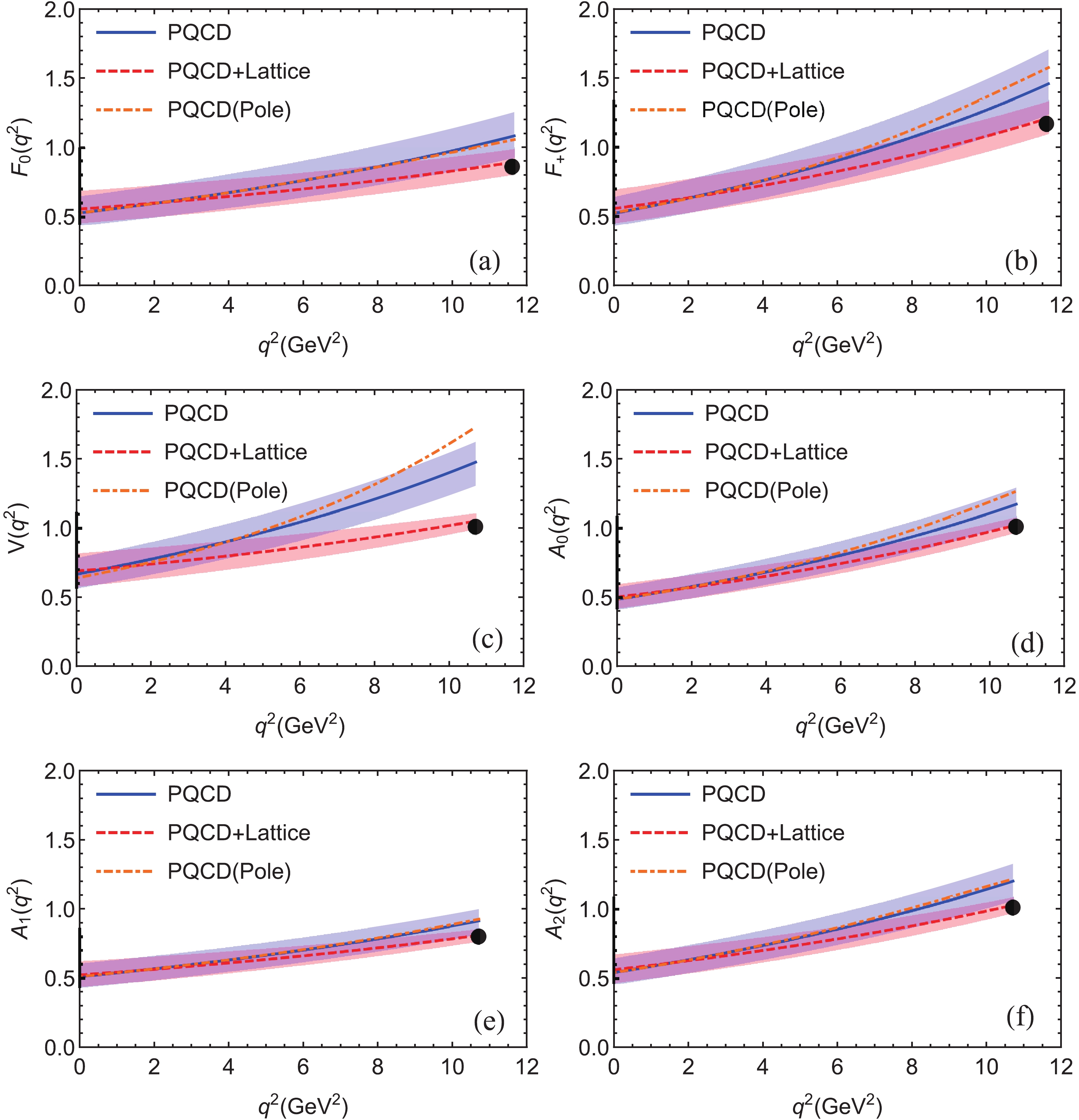
Figure 2. (color online) Theoretical predictions of the
q^2 dependence of the six form factors forB \to (D,D^{*}) transitions in the PQCD approach (blue solid curves) and the “PQCD+Lattice” method (red dashed curves) using the BCL parametrization [49, 50]. The orange dashed curves denote the PQCD predictions using the traditional pole model [9, 42, 58].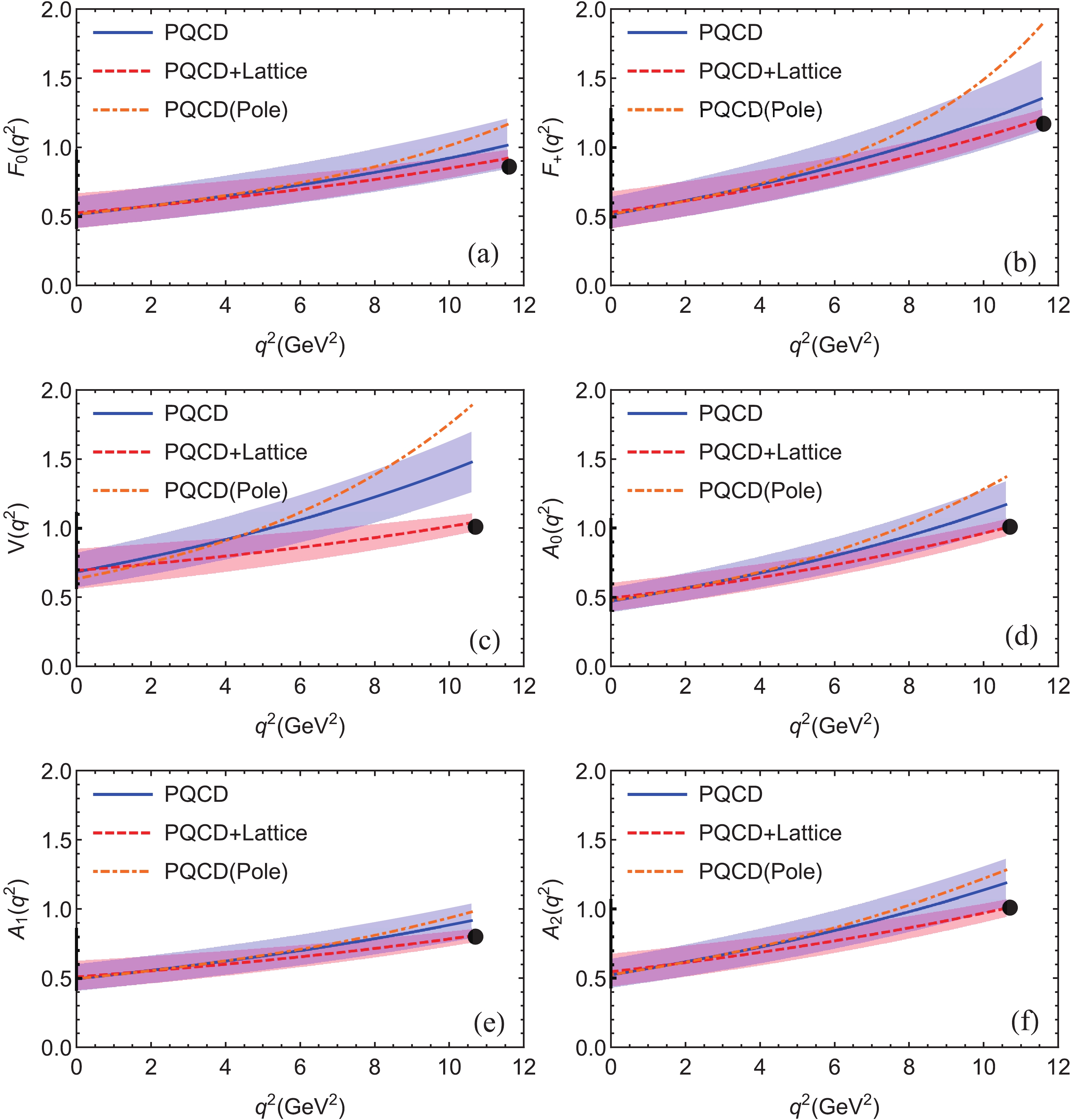
Figure 3. (color online) Theoretical predictions of the
q^2 dependence of the six form factors forB^0_s \to (D^-_s,D^{*-}_s) transitions in the PQCD approach (blue solid curves) and the “PQCD+Lattice” method (red dashed curves) using the BCL parametrization [49, 50]. The orange dashed curves denote the PQCD predictions using the traditional pole model [9, 42, 58].(1) The form factors forB\to D^{(*)} andB_s\to D_s^{(*)} transitions have very similar values in the wholeq^2 range due to the SU(3) flavor symmetry.(2) The differences between the theoretical predictions of the form factors in the traditional PQCD approach and the "PQCD+Lattice" method are small for lowq^2 and remain moderate for largeq^2 , in particular forF_{0,+}(q^2) andA_{0,1,2}(q^2) . ForV(q^2) , the difference is more pronounced for largeq^2 . For theB\to D^* transition, we foundV(10.71)\approx 1.53 (1.06 ) in the PQCD approach (“PQCD + Lattice” method). For theB_s\to D_s^* transition, we found a very similar result.(3) The difference between the PQCD predictions of the central values of the form factors obtained using the traditional pole model and the BCL model is very small in the regionq^2 < 8 GeV2. The largest differences in the region nearq^2_{\max} are\Delta F_+(11.55) = 0.59 (i.e, about 31% ofF_+(11.55) = 1.89 in the pole model), and\Delta V(10.59) = 0.36 (i.e. about 19% ofV(10.59) = 1.89 in the pole model) for theB_s \to D_s^{(*)} transition, as illustrated in Fig. 3. -
Inserting the obtained form factors in the differential decay rates given in Eqs. (40)-(43), it is straightforward to integrate over the range
m_l^2 \leqslant q^2 \leqslant (m_{B_{(s)}}-m_{D^{(*)}_{(s)}})^2 . For the four semileptonic decaysB^0_s \to D^{(*)}_s \tau^+\nu_\tau andB_s \to D^{(*)}_s l^+\nu_l withl^+ = (e^+,\mu^+) , the theoretical predictions of the branching ratios are the following:{\cal{B}}(B_s^0 \to D_s^ - {\tau ^ + }{\nu _\tau }){\rm{ }} = \left\{ {\begin{array}{*{20}{l}} {0.72_{ - 0.23}^{ + 0.32}({\omega _{{{{B}}_{\rm{s}}}}}) \pm 0.03({V_{{{cb}}}}) \pm 0.02({m_{\rm{c}}}),}&{{\rm{PQCD}},}\\ {0.63_{ - 0.13}^{ + 0.17}({\omega _{{{{B}}_{{s}}}}}) \pm 0.03({V_{{{cb}}}}) \pm 0.02({m_{{c}}}),}&{{\rm{PQCD + Lattice}},} \end{array}} \right.
(61) {\cal{B}}(B_s^0 \to D_s^ - {l^ + }{\nu _l}){\rm{ }} = \left\{ {\begin{array}{*{20}{l}} {1.97_{ - 0.65}^{ + 0.88}({\omega _{{{{B}}_{{s}}}}}) \pm 0.08({V_{{{cb}}}}) \pm 0.03({m_{{c}}}),}&{{\rm{PQCD}},}\\ {1.84_{ - 0.50}^{ + 0.76}({\omega _{{{{B}}_{{s}}}}}) \pm 0.08({V_{{{cb}}}}) \pm 0.03({m_{{c}}}),}&{{\rm{PQCD + Lattice}},} \end{array}} \right.
(62) {\cal{B}}(B_s^0 \to D_s^{* - }{\tau ^ + }{\nu _\tau }){\rm{ }} = \left\{ {\begin{array}{*{20}{l}} {1.45_{ - 0.39}^{ + 0.45}({\omega _{{{{B}}_{{s}}}}}) \pm 0.06({V_{{{cb}}}}) \pm 0.06({m_{{c}}}),}&{{\rm{PQCD}},}\\ {1.20_{ - 0.22}^{ + 0.25}({\omega _{{{{B}}_{{s}}}}}) \pm 0.05({V_{{{cb}}}}) \pm 0.02({m_{{c}}}),}&{{\rm{PQCD + Lattice}},} \end{array}} \right.
(63) {\cal{B}}(B_s^0 \to D_s^{* - }{l^ + }{\nu _l}) = \left\{ {\begin{array}{*{20}{l}} {5.04_{ - 1.41}^{ + 1.60}({\omega _{{{{B}}_{{s}}}}}) \pm 0.20({V_{{{cb}}}}) \pm 0.16({m_{{c}}}),}&{{\rm{PQCD}},}\\ {4.42_{ - 0.98}^{ + 1.26}({\omega _{{{{B}}_{{s}}}}}) \pm 0.17({V_{{{cb}}}}) \pm 0.06({m_{{c}}}),}&{{\rm{PQCD + Lattice}},} \end{array}} \right.
(64) where the theoretical errors come mainly from the uncertainties of the input parameters
\omega_{B_s} = 0.50 \pm 0.05 GeV,|V_{{cb}}| = (42.2 \pm 0.8) \times 10^{-3} andm_{c} = 1.275^{+0.025}_{-0.035} GeV. Errors from the uncertainties of the decay constants of the initialB_s and the finalD_s^{(*)} mesons are small and have been neglected. In Table 2, we list our PQCD and “PQCD+Lattice” predictions of the branching ratios of the semileptonic decays ofB_s^0 , where the total errors are obtained by adding the individual errors in quadrature. As a comparison, we also show predictions of some other theoretical approaches in the SM framework. Unfortunately, there are no experimental results available at present. In Table 3, we show the theoretical predictions of the ratios of the branching fractionsR(D_s) andR(D_s^*) defined in the same way asR(D^{(*)}) :Approach {\cal {B}}(B^0_s \to D^-_s l^+ \nu_l) 
{\cal {B}}(B^0_s \to D^-_s \tau^+ \nu_\tau) 
{\cal {B}}(B^0_s \to D^{*-}_s l^+ \nu_l) 
{\cal {B}}(B^0_s \to D^{*-}_s \tau^+ \nu_\tau) 
PQCD 1.97^{+0.89}_{-0.66} 
0.72^{+0.32}_{-0.23} 
5.04^{+1.62}_{-1.43} 
1.45^{+0.46}_{-0.40} 
PQCD+Lattice 1.84^{+0.77}_{-0.51} 
0.63^{+0.17}_{-0.13} 
4.42^{+1.27}_{-1.00} 
1.20^{+0.26}_{-0.23} 
PQCD[42] 2.13^{+1.12}_{-0.77} 
0.84^{+0.38}_{-0.28} 
4.76^{+1.87}_{-1.49} 
1.44^{+0.51}_{-0.42} 
IAMF[67] 1.4-1.7 
0.47-0.55 
5.1-5.8 
1.2-1.3 
RQM[68] 2.1\pm0.2 
0.62\pm0.05 
5.3\pm0.5 
1.3\pm0.1 
LCSR[69] 1.0^{+0.4}_{-0.3} 
0.33^{+0.14}_{-0.11} 
- 
- 
LFQM[70] - 
- 
5.2\pm0.6 
1.3^{+0.2}_{-0.1} 
CQM[71] 2.73-3.00 
- 
7.49-7.66 
- 
QCDSR[72] 2.8-3.8 
- 
1.89-6.61 
- 
Lattice[73] 2.013-2.469 
0.619-0.724 
- 
- 
\begin{split}R({D_s}) =& \frac{{{\cal{B}}(B_s^0 \to D_s^ - {\tau ^ + }{\nu _\tau })}}{{{\cal{B}}(B_s^0 \to D_s^ - {l^ + }{\nu _l})}} \\=& \left\{ {\begin{array}{*{20}{l}} {0.365_{ - 0.012}^{ + 0.009},}&{{\rm{PQCD}},}\\ {0.341_{ - 0.025}^{ + 0.024},}&{{\rm{PQCD + Lattice}},} \end{array}} \right. \end{split}
(65) \begin{split}R(D_s^*) = &\frac{{{\cal{B}}(B_s^0 \to D_s^{* - }{\tau ^ + }{\nu _\tau })}}{{{\cal{B}}(B_s^0 \to D_s^{* - }{l^ + }{\nu _l})}} \\=& \left\{ {\begin{array}{*{20}{l}} {0.287_{ - 0.011}^{ + 0.008},}&{{\rm{PQCD}},}\\ {0.271_{ - 0.016}^{ + 0.015},}&{{\rm{PQCD + Lattice}},} \end{array}} \right. \end{split}
(66) where l denotes an electron or a muon.
Following the same procedure as for
B_s decays, we calculate the branching ratios and the ratiosR(D^{(*)}) forB \to (D,D^*)(l^+ \nu_l, \tau^+ \nu_\tau) decays. The numerical results are listed in Table 4 for the branching ratios and in Table 5 for the ratiosR(D) andR(D^*) . In the estimate of the errors,\omega_{\rm {B}} = 0.40 \pm 0.04 GeV was used.Channels PQCD PQCD+Lattice PQCD[10] HQET[11] PDG[65] B^+ \to D^0 \tau^+ \nu_\tau 
0.86^{+0.34}_{-0.25} 
0.69^{+0.21}_{-0.17} 
0.95^{+0.37}_{-0.31} 
0.66\pm 0.05 
0.77\pm0.25 
B^+ \to D^0 l^+ \nu_l 
2.29^{+0.91}_{-0.72} 
2.10^{+0.85}_{-0.62} 
2.19^{+0.99}_{-0.76} 
- 
2.20\pm0.10 
B^+ \to D^{*0} \tau^+ \nu_\tau 
1.60^{+0.39}_{-0.37} 
1.34^{+0.26}_{-0.23} 
1.47^{+0.43}_{-0.40} 
1.43\pm 0.05 
1.88\pm0.20 
B^+ \to D^{*0} l^+ \nu_l 
5.53^{+1.45}_{-1.25} 
4.89^{+1.21}_{-1.00} 
4.87^{+1.60}_{-1.41} 
- 
4.88\pm0.10 
B^0 \to D^- \tau^+ \nu_\tau 
0.82^{+0.33}_{-0.24} 
0.62^{+0.19}_{-0.14} 
0.87^{+0.34}_{-0.28} 
0.64\pm 0.05 
1.03\pm0.22 
B^0 \to D^- l^+ \nu_l 
2.19^{+0.91}_{-0.68} 
1.95^{+0.77}_{-0.56} 
2.03^{+0.92}_{-0.70} 
- 
2.20\pm0.10 
B^0 \to D^{*-} \tau^+ \nu_\tau 
1.53^{+0.37}_{-0.35} 
1.25^{+0.25}_{-0.21} 
1.36^{+0.38}_{-0.37} 
1.29\pm 0.06 
1.67\pm0.13 
B^0 \to D^{*-} l^+ \nu_l 
5.32^{+1.37}_{-1.20} 
4.63^{+1.15}_{-0.95} 
4.52^{+1.44}_{-1.31} 
- 
4.88\pm0.10 
Table 4. PQCD and “PQCD+Lattice” predictions of the branching ratios (in units of
10^{-2} ) of the eight semileptonic decaysB \to D^{(*)} \tau^+ \nu_\tau andB \to D^{(*)} l^+ \nu_l withl = (e,\mu) . As a comparison, the previous “PQCD+Lattice” predictions [10], the SM predictions based on HQET [11], and the world average of the measured values given in PDG 2018 [65] are also shown.Table 5. PQCD and "PQCD+Lattice" predictions of the ratios
R(D) andR(D^*) . As a comparison, the previous "PQCD+Lattice" predictions given in Ref. [10], the average of the SM predictions given in Ref. [29], measured values reported by the BaBar, Belle and LHCb collaborations [1, 24, 25], and the world averaged results from HFLAV group [29] are also shown.From Tables 2 – 5, the following points can be noted:
(1) For the semileptonic decaysB\to D^{(*)}l^+ \nu_l withl = (e,\mu,\tau) , the “PQCD+Lattice” predictions of the branching ratios and the ratiosR(D^{(*)}) agree with the available experimental data within errors. This can be viewed as evidence of the reliability of the “PQCD+Lattice” method for calculating semileptonic decays of B meson.(2) For the fourB_s decay modes and the eight B decay modes, the "PQCD+Lattice" predictions of the branching ratios are generally smaller than the conventional PQCD predictions, but the differences are relatively small, less than 20%. The predictions also agree with the previous PQCD predictions given in Refs. [9, 10, 42] within the still large theoretical uncertainties.(3) For the ratiosR(D_s) andR(D_s^*) , the theoretical errors largely cancel, and the PQCD and "PQCD+Lattice" predictions have a very small error, only about 5%. These predictions could be tested in the near future by the LHCb and Belle-II experiments.(4) For the branching ratios, the predictions of the different theoretical approaches can be somewhat different for the same decay mode, but they still agree within errors, since the theoretical uncertainties are large. For the ratiosR(D) andR(D^*) , our “PQCD+Lattice” predictions agree with the average of the SM predictions obtained by HQET and the lattice QCD input for the form factors [3–6, 29].(5) Comparing the two sets of ratios(R(D), R(D_s)) and(R(D^*),R(D_s^*)) , listed in Tables 3 and 5, one can see that the SU(3) flavor symmetry is well preserved in the PQCD and the "PQCD+Lattaice" approaches. This point could also be tested by experiments. -
Besides the branching ratios and the ratios
R(X) , we consider three additional physical observables: the longitudinal polarization of the tau leptonP_\tau(D_{(s)}^{(*)}) , the fraction ofD_{(s)}^* longitudinal polarizationF_L(D_{(s)}^*) and the forward-backward asymmetry of the tau leptonA_{FB}(\tau) . These quantities could be measured by the LHCb and Belle experiments, and may be sensitive to new physics [2, 31, 61–63]. Investigation of these physical observables may provide new clues for understanding theR(D^{(*)}) puzzle, and it is therefore necessary and interesting to calculate them.In Refs. [31–33], these three physical observables were calculated in the SM framework, and possible new physics effects were studied. We calculate these observables in the PQCD and “PQCD+Lattice” approaches using Eqs. (44)-(59), and show the numerical predictions of
P_\tau(D_{(s)}^{(*)}) ,F_L(D_{(s)}^*) andA_{FB}(\tau) in Table 6. The measured values ofP_{\tau}(D^*) andF_L(D^*) [20, 21, 30] given in Eqs. (4), (5) are also listed in Table 6. As a comparison, we also show the SM predictions of these physical observables given in Refs. [31, 32] .Observable Approach B^0\to D^- \tau^+\nu_\tau 
B^0_s\to D^-_s \tau^+ \nu_\tau 
B^0\to D^{*- } \tau^+ \nu_\tau 
B^0_s\to D_s^{*-} \tau^+ \nu_l 
P_\tau(D_{(s)}^{(*)}) 
PQCD 0.32(1) 
0.31(1) 
-0.54(1) 
-0.54(1) 
PQCD+Lat. 0.30(1) 
0.30(1) 
-0.53(1) 
-0.53(1) 
SM[31] - 
- 
-0.497(13) 
- 
SM[32] 0.325(3) 
- 
-0.508(4) 
- 
Belle[20] - 
- 
-0.38\pm 0.51^{+0.21}_{-0.16} 
- 
F_{\rm L}(D_{(s)}^*) 
PQCD - 
- 
0.42(1) 
0.42(1) 
PQCD+Lat. - 
- 
0.43(1) 
0.43(1) 
SM[33] - 
- 
0.457(10) 
- 
SM[32] - 
- 
0.441(6) 
- 
Belle[30] - 
- 
0.60\pm 0.08\pm 0.04 
- 
A_{\rm FB}(\tau) 
PQCD 0.35(1) 
0.36(1) 
-0.085(2) 
-0.083(2) 
PQCD+Lat. 0.36(1) 
0.36(1) 
-0.054(2) 
-0.050(2) 
SM[32] 0.361(1) 
- 
-0.084(13) 
- 
Table 6. PQCD and "PQCD+Lattice" predictions of
P_\tau(D_{(s)}^{(*)}) ,F_L(D_{(s)}^*) andA_{FB}(\tau) . The SM predictions and the measured values are also listed.From the results listed in Eqs. (4), (5) and in Table 6, the following points can be noted:
(1) The uncertainties of the theoretical predictions of the physical observablesP_\tau(D_{(s)}^{(*)}) ,F_L(D_{(s)}^*) andA_{FB}(\tau) are very small compared to the branching ratios, since the theoretical uncertainties largely cancel in the ratios.(2) The PQCD and “PQCD+Lattice” predictions of the physical observablesP_\tau(D_{(s)}^{(*)}) ,F_L(D_{(s)}^*) andA_{FB}(\tau) forB_{(s)} \to D_{(s)}\tau^+ \nu_\tau decays are very similar: the difference for a fixed decay mode is less than 5%. ForA_{FB}(\tau) of theB_{(s)} \to D^*_{(s)} \tau^+\nu_\tau decays, however, the difference is about 40%. The reason is the definition of the angular coefficient functionb^{(D^*)}_\theta(q^2) , where the term(H_{V,+}^2-H_{V,-}^2) in Eq. (59) can be moderately changed by the highq^2 behavior of the form factors in the PQCD and “PQCD+Lattice” approaches. Clearly, a precise experimental measurement of the forward-backward asymmetryA_{FB}(\tau) in theB_{(s)} \to D^*_{(s)} l^+\nu_l decays could be of great help to test and improve the factorization models.(3) ForP_\tau(D^*) andF_L(D^*) , our theoretical predictions agree with the measured data within errors, partially due to the still large experimental errors. For all decay modes considered, the PQCD and “PQCD+Lattice” predictions of the three physical observables are consistent with the other approaches in the SM framework. We expect that these physical observables could be measured with high precision in the future by the LHCb and Belle-II experiments, which could help to test the theoretical models or approaches. -
In this paper, we studied the semileptonic decays
B_{(s)} \to D_{(s)}^{(*)} l^+ \nu_l in the SM framework by employing the conventional PQCD factorization approach and the “PQCD+Lattice” approach. In the second approach, we took into account the lattice QCD results of the relevant form factors as input for the extrapolation from the lowq^2 to the endpointq^2_{\max} . We calculated the form factorsF_{\rm 0,+}(q^2) ,V(q^2) andA_{\rm 0,1,2}(q^2) of theB_{(s)} \to D_{(s)}^{(*)} transitions, provided the theoretical predictions of the branching ratios of theB/B_s semileptonic decays and of the ratiosR(D^{(*)}) andR(D_s^{(*)}) . In addition, we also gave our theoretical predictions of the additional physical observables: the longitudinal polarization of the tau leptonP_\tau(D_{(s)}^{(*)}) , the fraction ofD_{(s)}^* longitudinal polarizationF_L(D_{(s)}^*) and the forward-backward asymmetry of the tau leptonA_{FB}(\tau) .From the numerical calculations and phenomenological analysis we noted the following points:
(1) For the twelveB/B_s semileptonic decay modes considered, the "PQCD+Lattice" predictions of the branching ratios are generally smaller than the conventional PQCD predictions, but the differences are relatively small, less than 20%. The “PQCD+Lattice” predictions of the branching ratios and the ratiosR(D^{(*)}) agree with the available experimental measurements within errors.(2) For the ratiosR(D_s) andR(D_s^*) , the PQCD and "PQCD+Lattice" predictions are the following:R({D_s}) = \left\{ {\begin{array}{*{20}{l}} {0.365_{ - 0.012}^{ + 0.009},}&{{\rm{PQCD}},}\\ {0.341_{ - 0.025}^{ + 0.024},}&{{\rm{PQCD + Lattice}},} \end{array}} \right.
(67) R(D_s^*) = \left\{ {\begin{array}{*{20}{l}} {0.287_{ - 0.011}^{ + 0.008},}&{{\rm{PQCD}},}\\ {0.271_{ - 0.016}^{ + 0.015},}&{{\rm{PQCD + Lattice}}.} \end{array}} \right.
(68) They agree with the other SM predictions based on different approaches. These predictions could be tested by the LHCb and Belle-II experiments.
(3) For most of the observablesP_\tau(D_{(s)}^{(*)}) ,F_L(D_{(s)}^*) andA_{FB}(\tau) , the PQCD and “PQCD+Lattice” predictions agree, and the difference is less than 5%. The relatively large difference ofA_{FB}(\tau) in theB_{(s)} \to D^*_{(s)} \tau^+\nu_\tau decays can be reasonably explained.(4) ForP_\tau(D^*) andF_L(D^*) , our theoretical predictions agree with the measurements within errors. For all decay modes considered, the PQCD and “PQCD+Lattice” predictions of these physical observables are consistent with the results of the other approaches in the SM framework. The LHCb and Belle-II experiments could help to test the above theoretical predictions.We wish to thank Wen-Fei Wang and Ying-Ying Fan for valuable discussions.
-
In this appendix, we present the explicit expressions for some functions which have already appeared in the previous sections. The hard functions
h_1 andh_2 come form the Fourier transform and can be written as:\tag{A1} \begin{split} h_1(x_1,x_2,b_1,b_2) =& K_0(\beta_1 b_1) [\theta(b_1-b_2)I_0(\alpha_1 b_2)K_0(\alpha_1 b_1)\\ &+\theta(b_2-b_1)I_0(\alpha_1 b_1)K_0(\alpha_1 b_2)]S_t(x_2), \end{split}
\tag{A2} \begin{split} h_2(x_1,x_2,b_1,b_2) =& K_0(\beta_2 b_1) [\theta(b_1-b_2)I_0(\alpha_2 b_2)K_0(\alpha_2 b_1)\\ &+\theta(b_2-b_1)I_0(\alpha_2 b_1)K_0(\alpha_2 b_2)]S_t(x_2), \end{split}
where
K_0 andI_0 are the modified Bessel functions, and\tag{A3} \alpha_1 = m_{B_{(s)}}\sqrt{x_2r \eta^+},\quad \alpha_2 = m_{B_{(s)}}\sqrt{x_1 r \eta^+ - r^2+r_c^2},\quad \beta_1 = \beta_2 = m_{B_{(s)}}\sqrt{x_1x_2 r \eta^+}.
The threshold resummation factor
S_t(x) is adopted from Ref. [74]:\tag{A4} S_t = \frac{2^{1+2c}\Gamma(3/2+c)}{\sqrt{\pi}\Gamma(1+c)}[x(1-x)]^c,
and here we use
c = 0.3 .The factor
\exp[-S_{ab}(t)] contains the Sudakov logarithmic corrections and the renormalization group evolution effects of the wave functions and the hard scattering amplitude withS_{ab}(t) = S_B(t)+S_M(t) [74, 75],\tag{A5} S_B(t) = s\left(x_1\frac{m_{B_{(s)}}}{\sqrt{2}},b_1\right) +\frac{5}{3}\int_{1/b_1}^{t}\frac{{\rm d}\bar{\mu}}{\bar{\mu}}\gamma_q(\alpha_s(\bar{\mu})),
\tag{A6} \begin{split} S_M(t) =& s\left (x_2\frac{m_{B_{(s)}}}{\sqrt{2}} r\eta^+,b_2 \right) +s\left ((1-x_2)\frac{m_{B_{(s)}}}{\sqrt{2}} r \eta^+,b_2 \right) \\&+2\int_{1/b_2}^{t}\frac{{\rm d}\bar{\mu}}{\bar{\mu}} \gamma_q(\alpha_s(\bar{\mu})), \end{split}
where
\eta^+ is defined in Eq. (7). The hard scale t and the quark anomalous dimension\gamma_q = -\alpha_s/\pi govern the aforementioned renormalization group evolution. The explicit expressions for the functionss(Q,b) can be found in Appendix A of Ref. [75]. The hard scalest_i in Eqs. (22)-(27) are chosen as the largest scales of virtuality of internal particles in the hard b quark decay diagram,\begin{align} t_1& = \max\{m_{B_{(s)}}\sqrt{x_2 r \eta^+}, 1/b_1, 1/b_2\}, \\ t_2& = \max\{m_{B_{(s)}}\sqrt{x_1 r \eta^+ - r^2+r_c^2},1/b_1, 1/b_2\}. \end{align}
(A7)
Semileptonic decays B/Bs→(D(∗),D(∗)s)lνl in the PQCD approach with the lattice QCD input
- Received Date: 2019-12-09
- Available Online: 2020-05-01
Abstract: We study the semileptonic


 DownLoad: