


 Abstract
 HTML
HTML Reference
 Related
 PDF
PDF


-
Nucleon structure is one of the hottest research topics in hadron physics, and has attracted considerable experimental and theoretical effort. With the upgrade of the experimental facilities, more information about the structure of the nucleon will become available. By increasing the energy, experimentalists can obtain the parton distribution functions (PDFs) from deep inelastic scattering, as well as the form factors at relatively large momentum transfer from elastic scattering. In addition to the valence quark, both the analytical and numerical information about the sea quark contribution to nucleon properties is also very important, as it is crucial for determining the leading non-analytic behavior of physical quantities.
The strange quark contribution to the nucleon form factor is of special interest because it is purely from sea quarks. Experiments by different collaborations have been carried out to measure this quantity precisely [1-4]. There have also been many theoretical discussions of the strange quark form factors [5-7]. In 2002, we studied the strange quark form factors with the perturbative chiral quark model (PCQM), and it was found that the strange quark electric form factor is positive while the magnetic form factor is negative [8]. At that time, the theoretical predictions were quite different as there were no precise experimental measurements available.
It is impossible to study the nucleon structure using quantum chromodynamics directly because of its non-perturbative nature. Besides the phenomenological quark models, two methods are systematically used in hadron physics, the lattice simulations and the effective field theory or the chiral perturbation theory. Traditionally, the chiral perturbation theory with dimensional regularization (DR) is valid only at low momentum transfer
$ Q^2 < 0.1 $ GeV2 [9]. It can be applied up to 0.4 GeV2 if vector mesons are included [10]. In lattice simulations, many quantities simulated on the lattice are for large quark (pion) mass, and it is necessary to extrapolate the lattice results to the physical pion mass. Instead of DR, we applied the effective field theory with finite range regularization (FRR). The vector meson mass, magnetic moments, magnetic form factors, strange quark form factors, charge radii, first moments of GPDs, nucleon spin etc., could be successfully extrapolated to the physical mass [11-20]. The strange quark form factors obtained with FRR are also consistent with our previous results with PCQM [12, 15]. Recently, the nucleon form factors, as well as the sea contribution of the light and strange quarks, were simulated on the lattice for the physical pion mass [21-24]. Therefore, it would be interesting to compare these result with those calculated in the framework of the effective field theory.In recent years, we proposed a nonlocal chiral effective Lagrangian which makes it possible to study the hadron properties at relatively large
$ Q^2 $ [25-30]. The nonlocal interaction generates both the regulator which makes the loop integral convergent, and the$ Q^2 $ dependence of the form factors at tree level. The obtained electromagnetic form factors and strange quark form factors of the nucleon are very close to the experimental data [28, 29]. In this paper, we apply the nonlocal Lagrangian to investigate the light sea quark contribution to the nucleon form factors. With the quark flow method as in Ref. [30], we obtain the sea and valence quark contributions separately. This method is equivalent to the quenched chiral perturbation theory. In Sec. 2, we introduce the nonlocal chiral Lagrangian. The sea quark contributions to the nucleon form factors are derived in Sec. 3. Numerical results are shown in Sec. 4, and finally, a short summary is given in Sec. 5. -
The lowest order chiral Lagrangian for baryons, pseudo-scalar mesons and their interactions can be written as [28, 31-33],
$ \begin{split} {\cal{L}} = & {\rm i}\,{\rm Tr}\,{\bar{B}} \gamma_{\mu}\,{\not\!\!{\cal{D}}}B -m_B\,{\rm Tr}\,{\bar{B}}B \\ &+{\bar{T}}_\mu^{abc}(i\gamma^{\mu\nu\alpha}D_\alpha\,-\,m_T\gamma^{\mu\nu}) T_\nu^{abc} \\& +\frac{f^2}{4}{\rm Tr}\,\partial_\mu\Sigma\,\partial^\mu\Sigma^\dagger +D\,{\rm Tr}\, {\bar{B}} \gamma_\mu \gamma_5\, \{A_\mu,B\} \\& +F\,{\rm Tr}\, {\bar{B}} \gamma_\mu \gamma_5\, [A_\mu,B] \\& +\left [\frac{C}{f}\epsilon^{abc}{\bar{T}}_\mu^{ade} (g^{\mu\nu}+z\gamma_\mu\gamma_\nu) B_c^e\partial_\nu\phi_b^d+H.C \right ], \end{split} $

(1) where D, F and C are the coupling constants. The chiral covariant derivative
$ {\cal{D}}_\mu $ is defined as$ {\cal{D}}_\mu B = \partial_\mu B+[V_\mu,B] $ . The pseudo-scalar meson octet couples to the baryon field via the vector and axial vector combinations as$ \begin{align} &V_\mu = \frac12(\zeta\partial_\mu\zeta^\dagger+\zeta^\dagger\partial_\mu\zeta)+\frac{1}{2}{\rm i}e{\cal{A}}^\mu (\zeta^\dagger\,Q_c\,\zeta+\zeta\,Q_c\,\zeta^\dagger), \\ &A_\mu = \frac12(\zeta\partial_\mu\zeta^\dagger-\zeta^\dagger\partial_\mu\zeta)-\frac{1}{2}e{\cal{A}}^\mu (\zeta\,Q_c\,\zeta^\dagger-\zeta^\dagger\,Q_c\,\zeta), \end{align} $

(2) where
$ \zeta^2 = \Sigma = {\rm e}^{{\rm i}2\phi/f},\qquad f = 93\; {\rm {MeV}}. $

(3) $ Q_c $ is the real charge matrix$ {\rm{diag}} (2/3,-1/3,-1/3) $ .$ \phi $ and B are the matrices of pseudo-scalar fields and octet baryons.$ {\cal{A}}^\mu $ is the photon field. The covariant derivative$ D_\mu $ in the decuplet sector is defined as$ D_\nu T_\mu^{abc} =\partial_\nu T_\mu^{abc}+ $ $ (\Gamma_\nu,T_\mu)^{abc} $ , where$ \Gamma_\nu $ is the chiral connection defined as$ (X,T_\mu) = (X)_d^aT_\mu^{dbc}+(X)_d^bT_\mu^{adc}+(X)_d^cT_{\mu}^{abd} $ .$ \gamma^{\mu\nu\alpha} $ ,$ \gamma^{\mu\nu} $ are the antisymmetric matrices expressed as$ \gamma^{\mu\nu} = \frac12\left[\gamma^\mu,\gamma^\nu\right]\quad {\rm{and}}\quad \gamma^{\mu\nu\rho} = \frac14\left\{\left[\gamma^\mu,\gamma^\nu\right], \gamma^\rho\right\}.\, $

(4) The octet, decuplet and octet-decuplet transition magnetic moment operators are needed in the one loop calculations of the nucleon electromagnetic form factors. The baryon octet anomalous magnetic Lagrangian is written as
$ \begin{split} {\cal{L}}_{\rm oct} =& \frac{e}{4m_B}\Big( c_1\, \,{{\rm{Tr}}}\left[{\bar{B}} \sigma^{\mu\nu} \left\{F^+_{\mu\nu},B\right\}\right] + c_2\, \,{{\rm{Tr}}}\left[{\bar{B}}\sigma^{\mu\nu} \left[F^+_{\mu\nu},B \right]\right] \\ &+c_3\, \,{{\rm{Tr}}}\left[{\bar{B}}\sigma^{\mu\nu}B\right]\, \,{{\rm{Tr}}}\left[F^+_{\mu\nu},B\right] \Big), \end{split} $

(5) where,
$ F^\dagger_{\mu\nu} = -\frac12\left(\zeta^\dagger F_{\mu\nu}\,Q_c\,\zeta+\zeta F_{\mu\nu}\,Q_c\,\zeta^\dagger\right). $

(6) At the lowest order, the contribution of quark q to the nucleon magnetic moments can be obtained by replacing the charge matrix
$ Q_c $ with the corresponding diagonal quark matrices$ \lambda_q = {\rm{diag}}(\delta_{qu}, \delta_{qd}, \delta_{qs}) $ . After expansion of the above equation, it is found that$ \begin{align} F_2^{p,u} = {}&c_1+c_2+c_3,\qquad& F_2^{n,u} = {}&c_3,\\ F_2^{p,d} = {}&c_3,\qquad& F_2^{n,d} = {}&c_1+c_2+c_3,\\ F_2^{p,s} = {}&c_1-c_2+c_3,\qquad& F_2^{n,s} = {}&c_1-c_2+c_3.\\ \end{align} $

(7) Comparing with the results of the constituent quark model where
$ \begin{align} F_2^{p,s} = {}& 0 \; \; {\rm {and}}\; \; F_2^{n,s} = 0, \\ \end{align} $

(8) we get
$ {{{c}}_3} = {{{c}}_2}-{{{c}}_1}. $

(9) The transition magnetic operator is
$ \begin{split} {\cal{L}}_{\rm tr} =& {\rm i}\frac{e}{4m_N}\mu_T F_{\mu\nu} \Big( \epsilon^{ijk} Q_c^{il}{\bar{B}}^{jm}\gamma^\mu\gamma_5\, T^{\nu,klm} \\ &+ \epsilon^{ijk} Q_c^{li}{\bar{T}}^{\mu,klm}\,\gamma^\nu\gamma_5\,B^{mj} \Big). \end{split} $

(10) The effective decuplet anomalous magnetic moment operator can be expressed as
$ {\cal{L}}_{\rm dec} = -\frac{{\rm i}eF_2^T}{4M_T}{\bar{T}}_\mu^{abc}\sigma^{\rho\lambda}F_{\rho\lambda}T^{\mu,abc}. $

(11) The anomalous magnetic moments of baryons can also be expressed in terms of quark magnetic moments
$ \mu_q $ . For example,$ \mu_p = \frac43 \mu_u - \frac13 \mu_d $ ,$ \mu_n = \frac43 \mu_d - \frac13 \mu_u $ ,$ \mu_{\Delta^{++}} = 3\mu_u $ . Using the SU(3) symmetry,$ \mu_u = -2\mu_d = -2\mu_s $ ,$ \mu_T $ and$ F_2^T $ as well as$ \mu_q $ can be written in terms of$ c_1 $ or$ c_2 $ . For example,$ \mu_u = \frac23 c_1 $ ,$ \mu_T = 4 c_1 $ ,$ F_2^{\Delta^{++}} = \mu_{\Delta^{++}}-2 = 2c_1-2 $ .The gauge invariant nonlocal Lagrangian can be obtained using the method given in [26, 28, 29]. For instance, the local interaction including the
$ \pi $ meson can be written as$ {\cal{L}}_{\pi}^{\rm local} = \int\!\,{\rm d}x \frac{D+F}{\sqrt{2}f} \bar{p}(x)\gamma^\mu\gamma_5\,n(x)(\partial_\mu+{\rm i}e\,{\cal{A}}_\mu(x)) \pi^+(x). $

(12) The corresponding nonlocal Lagrangian is expressed as
$\begin{split} {\cal L}_{\pi}^{nl}= &\int\!\,{\rm d}x\int\!\,{\rm d}y\frac{D+F}{\sqrt{2}f}\bar{p}(x)\gamma^\mu\gamma_5 n(x)F(x-y)\\ &\times {\rm{exp}}\left[{\rm i}e\int_x^y {\rm d}z_\nu\int\!\,{\rm d}a\,{\cal{A}}^\nu(z-a)F(a)\right] \\ &\times \left(\partial_\mu\,+{\rm i}e\int\!\,{\rm d}a\,{\cal{A}}_\mu(y-a)F(a)\right)\pi^+(y), \end{split}$

(13) where
$ F(x) $ is the correlation function. To guarantee gauge invariance, the gauge link is introduced in the above Lagrangian. The regulator can be generated automatically with the correlation function.With the same procedure, the nonlocal electromagnetic interaction can also be obtained. For example, the local interaction between the proton and photon is written as
$ \begin{split} {\cal L}_{\rm EM}^{\rm local} =& -e \bar{p}(x) \gamma^\mu p(x) {\cal{A}}_\mu(x) s \\& +\frac{(c_1-1)e}{4m_N} \bar{p}(x)\sigma^{\mu\nu}p(x)F_{\mu\nu}(x). \end{split} $

(14) The corresponding nonlocal Lagrangian is expressed as
$ \begin{split} {\cal L}_{\rm EM}^{nl} =& -e \int {\rm d}a \bar{p}(x) \gamma^\mu p(x) {\cal{A}}_\mu(x-a)F_1(a) \\& + \frac{(c_1-1)e}{4m_N}\int {\rm d}a \bar{p}(x)\sigma^{\mu\nu}p(x)F_{\mu\nu}(x-a)F_2(a), \end{split} $

(15) where
$ F_1(a) $ and$ F_2(a) $ are the correlation functions for the nonlocal electric and magnetic interactions.The form factors at tree level which are momentum dependent can be easily obtained with the Fourier transformation of the correlation function. As in our previous work [28, 29], the correlation function is chosen such that the charge and magnetic form factors at tree level have the same momentum dependence as the nucleon-pion vertex, i.e.
$ G_M^{\rm tree}(q) = c_1G_E^{\rm tree}(q) = c_1\tilde{F}(q) $ , where$ \tilde{F}(q) $ is the Fourier transformation of the correlation function$ F(a) $ . The corresponding functions$ \tilde{F}_1(q) $ and$ \tilde{F}_2(q) $ are then expressed as$ \tilde{F}_1^p(q) = \tilde{F}(q)\frac{4m_N^2+c_1Q^2}{4m_N^2+Q^2},\; \; \; \tilde{F}_2^p(q) = \tilde{F}(q)\frac{4m_N^2}{4m_N^2+Q^2}, $

(16) where
$ Q^2 = -q^2 $ is the momentum transfer. From Eq. (13), two kinds of couplings between hadrons and photons can be obtained. One is the normal coupling, expressed as$ \begin{split} {\cal L}^{\rm nor} =& {\rm i}e\int\!\,{\rm d}x\int\!\,{\rm d}y\frac{D+F}{\sqrt{2}f}\bar{p}(x)\gamma^\mu\gamma_5 n(x)F(x-y)\pi^+(y) \\& \times \int\!\,{\rm d}a\,{\cal{A}}_\mu(y-a)F(a). \end{split} $

(17) This interaction is similar to the traditional local Lagrangian except for the correlation function. The other is the additional interaction obtained by the expansion of the gauge link, expressed as
$ \begin{split} {\cal L}^{\rm add} =& {\rm i}e\int\!\,{\rm d}x\int\!\,{\rm d}y\frac{D+F}{\sqrt{2}f}\bar{p}(x)\gamma^\mu\gamma_5 n(x)F(x-y) \\& \times \int_x^y {\rm d}z_\nu\int\!\,{\rm d}a\,{\cal{A}}^\nu(z-a)F(a)\partial_\mu \pi^+(y) . \end{split} $

(18) -
The contribution of the quark flavor f
$ (f = u,d,s) $ to the Dirac and Pauli form factors of the nucleon are defined as$ \begin{split} &< N(p^\prime)|J_\mu^f|N(p)> = \bar{u}(p^\prime) \left\{ \gamma^\mu F_1^{f}(Q^2)+ \frac{{\rm i}\sigma^{\mu\nu} q_\nu}{2m_N}F_2^{f}(Q^2) \right\}u(p), \end{split} $

(19) where
$ q = p^\prime-p $ . The electromagnetic form factors are defined as combinations of the above form factors for each flavor as$ \begin{align} G_E^{f}(Q^2) &{} = F_1^{f}(Q^2)-\frac{Q^2}{4m_N^2}F_2^{f}(Q^2),\\ G_M^{f}(Q^2) &{} = F_1^{f}(Q^2) +F_2^{f}(Q^2). \end{align} $

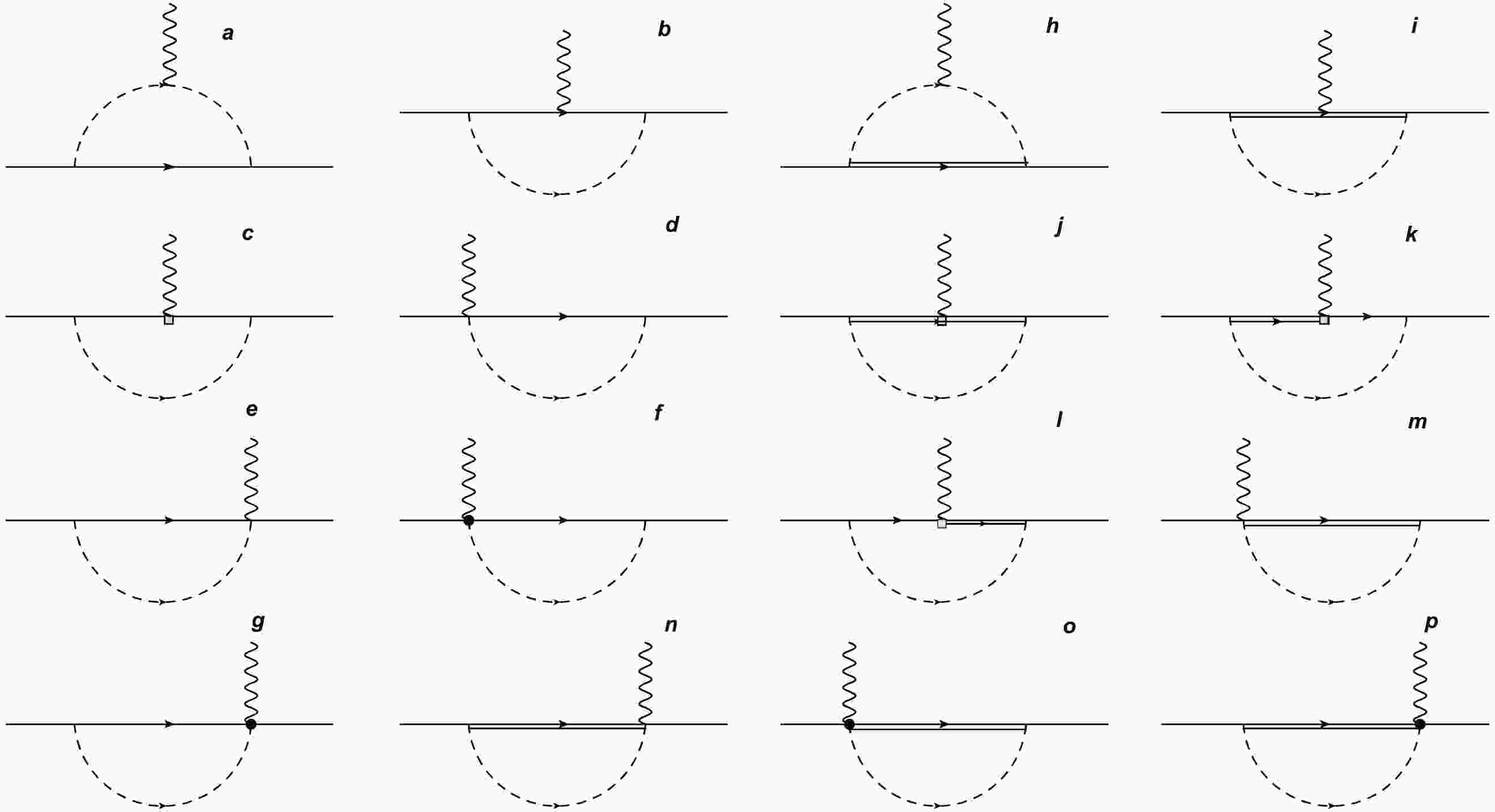
(20) In this work, we investigate the contribution of the u , d and s sea quarks to the nucleon electromagnetic form factors. According to the Lagrangian, the one loop Feynman diagrams which contribute to the nucleon electromagnetic form factors are shown in Fig. 1.
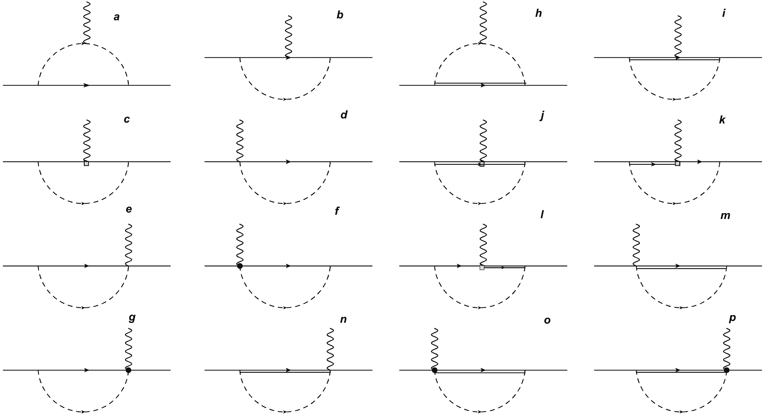
Figure 1. One loop Feynman diagrams for the nucleon electromagnetic form factors. The solid, double-solid, dashed and wave lines are for the octet baryons, decuplet baryons, pseudo-scalar mesons and photons, respectively. The rectangle and black dot represent the magnetic and additional interacting vertex.
The coupling constants between baryons and mesons (coefficients) in Fig. 1 can be obtained from the Lagrangian. For each diagram in Fig. 1, there exist quenched and disconnected diagrams. In order to obtain the pure sea quark contribution, we need to get the coefficients for the disconnected diagrams. The coefficients for the quenched and disconnected loop diagrams can be obtained separately as in Ref. [30], using the quark flows shown in Fig. 2. The obtained coefficients are the same as those extracted with the graded symmetry formalism in the quenched chiral perturbation theory [34]. In Fig. 2, we plot the
$ \pi^+ $ rainbow diagram using quark flows, as an example of the method of separating the quenched and sea quark contributions. The coefficients for the$ \pi^+ $ loop diagram in full QCD is$ (D+F)^2 $ . The coefficient in Fig. 2(b) for the sea quark contribution is the same as in Fig. 2(c) for the$ K^+ $ loop. The coefficient of the quenched sector can be obtained by subtracting the coefficient of the sea diagram from the total coefficient. The coefficients of u, d and s quarks for both quenched and sea quark flow diagrams are listed in Table 1. For$ \pi^0 $ , the first and second rows are for$ u\bar{u} $ and$ d\bar{d} $ , respectively.meson full QCD quenched diagram sea diagram $\pi^0$ 

$\frac{1}{2} (D+F)^2$ 

$-\frac{D^2}{3}+2 D F-F^2$ 

$\frac{D^2}{3}+F^2$ 

$\frac{1}{2} (D-F)^2$ 

$\pi^+$ 

$(D+F)^2$ 

$\frac{1}{3} \left(D^2+6 D F-3 F^2\right)$ 

$\frac{2}{3} \left(D^2+3 F^2\right)$ 

$\pi^-$ 

$0$ 

$-(D-F)^2$ 

$(D-F)^2$ 

$K^0$ 

$(D-F)^2$ 

$0$ 

$(D-F)^2$ 

$K^+$ 

$\frac{2}{3} \left(D^2+3 F^2\right)$ 

$0$ 

$\frac{2}{3} \left(D^2+3 F^2\right)$ 

Table 1. The coefficients for the quenched and sea diagrams and the total coefficients from Fig. 2.
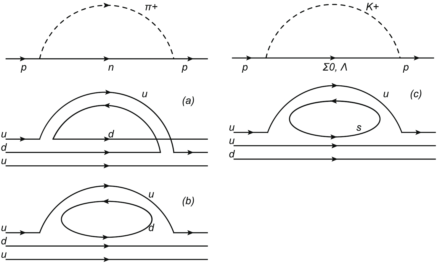
Figure 2. Quark flow diagrams for
$\pi^+$ and$K^+$ . (a) the quenched diagram; (b) and (c) the disconnected sea diagrams for$\pi^+$ and K, respectively.From the Lagrangian, we can get the matrix element of Eq. (19). In this section, we only show the expressions for the intermediate octet baryon. For the intermediate decuplet baryon, the expressions are similar but more complicated.
The sea quark contributions in Fig. 1a for u d and s quarks are written as
$ \Gamma_a^u = \left(\frac{4 D^2}{3}-2 D F+2 F^2\right) I_a^{N\pi},$

(21) $ \Gamma_a^d = \left(\frac{7 D^2}{6}-D F+\frac{5 F^2}{2}\right)I_a^{N\pi},$

(22) $ \Gamma_a^s = \frac{1}{6} (D+3 F)^2 I_a^{\Lambda K}+ \frac{3}{2} (D-F)^2 I_a^{\Sigma K}, $

(23) where the integral
$ I_a^{BM} $ is expressed as$ \begin{split} I_a^{BM} =& \frac{1}{2f^2}\bar{u}(p^\prime)\tilde F(q)\int\!\frac{{\rm d}^4 k}{(2\pi)^4}({\not\!{k}}+{\not\!{q}})\gamma_5\,\tilde F(q+k) \frac{1}{D_K(k+q)}\\&\times (2k+q)^\mu\frac{1}{D_M(k)}\frac{1}{{\not\!{p}}-{\not\!{k}}-m_B} (-{\not\!{k}}\gamma_5)\tilde F(k)u(p).\\[-15pt] \end{split} $

(24) $ D_M(k) $ is defined as$ D_M(k) = k^2-m_M^2+{\rm i}\epsilon. $

(25) $ m_B $ and$ m_M $ are the masses of the intermediate B baryon and M meson. The contributions in Fig. 1b are expressed as$ \begin{split} \Gamma_b^u =& \frac{2 {\rm i} m_B} {9 \left(4 m_B^2+Q^2\right)} \big[c_1 \left(-11 D^2+24 D F-9 F^2\right) \\ & +6 c_2 \left(2 D^2-3 D F+3 F^2\right)\big] I_b^{N \pi}, \end{split} $

(26) $ \begin{split} \Gamma_b^d = & -\frac{{\rm i} m_B}{9 \left(4 m_B^2+Q^2\right)} \big[c_1 \left(17 D^2-42 D F+9 F^2\right)\\ & -3 c_2 \left(7 D^2-6 D F+15 F^2\right) \big] I_b^{N \pi}, \end{split} $

(27) $ \begin{split} \Gamma_b^s = & \frac{{\rm i} \left(c_1+3 c_2\right) m_B (D+3 F)^2}{9 \left(4 m_B^2+Q^2\right)} I_b^{\Lambda \Lambda K} \\ & + \frac{3 {\rm i} \left(c_2-c_1\right) m_B (D-F)^2}{4 m_B^2+Q^2} I_b^{\Sigma K}, \end{split} $

(28) where the integral
$ I_b^{BM} $ is written as$ \begin{split} I_b^{BM} =& \frac{1}{2f^2}\bar{u}(p^\prime)\tilde F(q)\int\!\frac{{\rm d}^4 k}{(2\pi)^4}{\not\!{k}}\gamma_5\,\tilde F(k)\frac{1}{D_M(k)} \\ &\frac{1}{{\not\!\!{p'}}-{\not\!{k}}-m_B}\gamma^\mu \frac{1}{{\not\!\!{p}}-{\not\!{k}} -m_B}\frac{{\not\!{k}}\gamma_5}{\sqrt{2}f}\tilde F(k)u(p). \end{split} $

(29) Fig. 1c is similar to Fig. 1b, except for the magnetic interaction. The contributions of this diagram are written as
$ \begin{split} \Gamma_c^u = & \bigg(\frac{2 {\rm i} m_B \left(c_1 \left(-11 D^2+24 D F-9 F^2\right)\right)}{9 \left(4 m_B^2+Q^2\right)} \\ &+\frac{2 {\rm i} m_B \left(6 c_2 \left(2 D^2-3 D F+3 F^2\right)\right)}{9 \left(4 m_B^2+Q^2\right)} \bigg) I_c^{N \pi}, \end{split} $

(30) $ \begin{split} \Gamma_c^d =& \bigg(-\frac{{\rm i} m_B \left(c_1 \left(17 D^2-42 D F+9 F^2\right)\right)}{9 \left(4 m_B^2+Q^2\right)} \\ &+\frac{{\rm i} m_B \left(-3 c_2 \left(7 D^2-6 D F+15 F^2\right)\right)}{9 \left(4 m_B^2+Q^2\right)} \bigg) I_c^{N \pi}, \end{split} $

(31) $ \begin{split} \Gamma_c^s =& \frac{{\rm i} \left(c_1+3 c_2\right) m_B (D+3 F)^2}{9 \left(4 m_B^2+Q^2\right)} I_c^{\Lambda \Lambda K} \\ &+\frac{3 {\rm i} c_3 m_B (D-F)^2}{4 m_B^2+Q^2} I_c^{\Sigma K}, \end{split} $

(32) where
$ I_c^{\Lambda K} $ is expressed as$ \begin{split} I_c^{BM} =& \frac{1}{2f^2}\bar{u}(p^\prime)\tilde F(q)\int\!\frac{{\rm d}^4 k}{(2\pi)^4}{\not\!{k}}\gamma_5\tilde F(k) \frac{1}{{\not\!\!{p'}}-{\not\!{k}}-m_B} \\&\times \frac{\sigma^{\mu\nu}q_{\nu}}{2m_\Lambda} \frac{1}{{\not\!\!{p}}-{\not\!{k}}-m_B}\frac{\rm i}{D_M(k)} {\not\!{k}}\gamma_5\tilde F(k)u(p). \end{split} $

(33) Figures 1d and 1e are the Kroll-Ruderman diagrams. The contributions of these two diagrams are written as
$ \begin{align} \Gamma_{d+e}^u = {}& \left(-\frac{4 D^2}{3}+2 D F-2 F^2\right) I_{d+e}^{N \pi}, \end{align} $

(34) $ \begin{align} \Gamma_{d+e}^d = {}& \left(-\frac{7 D^2}{6}+D F-\frac{5 F^2}{2}\right) I_{d+e}^{N \pi}, \end{align} $

(35) $ \begin{align} \Gamma_{d+e}^s = {}& -\frac{1}{6} (D+3 F)^2 I_{d+e}^{\Lambda K} -\frac{3}{2} (D-F)^2 I_{d+e}^{\Sigma K}, \end{align} $

(36) where
$ \begin{split} I_{(d+e)}^{BM} = &\frac{1}{2f^2}\bar{u}(p^\prime)\tilde F(q)\int\!\frac{{\rm d}^4 k}{(2\pi)^4}{\not\!{k}}\gamma_5\tilde F(k) \frac{1}{{\not\!\!{p'}}-{\not\!{k}}-m_B} \\ &\times \frac{1}{D_M(k)}\gamma^\mu\gamma_5 \tilde F(k)u(p) \\ {}+{}&\frac{1}{2f^2}\bar{u}(p^\prime)\tilde F(q)\int\!\frac{{\rm d}^4 k}{(2\pi)^4}\gamma^\mu\gamma_5\tilde F(k)\frac{1}{{\not\!\!{p}}-{\not\!{k}}-m_B} \\ &\times \frac{1}{D_M(k)}{\not\!{k}}\gamma_5\tilde F(k)u(p). \end{split} $

(37) Figures 1f and 1g are the additional diagrams which are generated from the expansion of the gauge link terms. The contributions of these two diagrams for intermediate octet hyperons are expressed as
$ \Gamma_{f+g}^u = \left(-\frac{4 D^2}{3}+2 D F-2 F^2\right) I_{f+g}^{N \pi}, $

(38) $ \Gamma_{f+g}^d = \left(-\frac{7 D^2}{6}+D F-\frac{5 F^2}{2}\right) I_{f+g}^{N \pi} , $

(39) $ \Gamma_{f+g}^s =-\frac{1}{6} (D+3 F)^2 I_{f+g}^{\Lambda K} -\frac{3}{2} (D-F)^2 I_{f+g}^{\Sigma K},$

(40) where
$ \begin{split} I_{f+g}^{BM} =& \frac{1}{2f^2}\,\bar{u}(p^\prime)\tilde F(q)\int\!\frac{{\rm d}^4 k}{(2\pi)^4}{\not\!{k}}\gamma_5\tilde F(k)\frac{1}{{\not\!\!{p'}} -{\not\!{k}}-m_B} \\ &\times \frac{1}{D_M(k)}(-{\not\!{k}}+{\not\!\!{q}})\gamma_5\frac{(2k-q)^\mu}{2kq-q^2} [\tilde F(k-q)-\tilde F(k)]u(p) \\ & +\frac{1}{2f^2}\bar{u}(p^\prime)\tilde F(q)\int\!\frac{{\rm d}^4 k}{(2\pi)^4}({\not\!{k}}+{\not\!\!{q}})\gamma_5\frac{(2k+q)^\mu}{2kq+q^2} \\ &\times[\tilde F(k+q)-\tilde F(k)] \frac{1}{{\not\!\!{p}}-{\not\!{k}}-m_B} \frac{1}{D_M(k)}{\not\!{k}}\gamma_5F(k)u(p). \end{split} $

(41) Using Package-X [35] to simplify the
$ \gamma $ matrix algebra, we can get the expressions for the Dirac and Pauli form factors. In the next section, we discuss the numerical results. -
In the numerical calculations, the parameters are chosen as
$ D = 0.76 $ and$ F = 0.50 $ ($ g_A = D+F = 1.26 $ ). The coupling constant$ {C} $ is chosen as 1, the same as in Refs. [28, 36]. The off-shell parameter z is$ z = -1 $ [37]. The low energy constants$ c_1 $ and$ c_2 $ are determined as$ 2.057 $ and$ 0.748 $ , giving the experimental moments$ \mu_p = 2.793 $ and$ \mu_n = -1.913 $ . The covariant regulator is of the dipole form [28, 29, 31]$ \tilde{F}[k] = \frac{\Lambda^4}{(\Lambda^2+m_j^2-k^2)^2}, $

(42) where
$ m_j $ is the meson mass for the baryon-meson interaction and is zero for the hadron-photon interaction. It was found that for$ \Lambda $ around 0.90$ {\rm{GeV}} $ , the results are very close to the experimental nucleon form factors.In Fig. 3, we plot the sea contribution of the u quark with unit charge to the proton electric form factor. The three blue lines from top to bottom are for
$ \Lambda = 1.0,\; 0.9 $ and$ 0.8\; {\rm{GeV}} $ . As a comparison, the central result for the strange quark is also plotted in the figure with the red line. The solid dots with error bars are the lattice simulations from Ref. [22]. Since we do not include the valence contribution of the u quark in the proton, the electric form factor of the u quark is zero for$ Q^2 = 0 $ . It then increases with increasing$ Q^2 $ . For$ Q^2 $ larger than about 0.3$ {\rm{GeV}}^2 $ , it deceases with$ Q^2 $ . From the figure, one can see that the strange quark form factor can be described very well. The u quark result is slightly smaller than the lattice simulations. We should mention that the lattice results are for the light quarks and it was assumed that u and d have the same sea contributions. Therefore, the lattice results for the light quarks can be approximately treated as an average of the u and d contributions.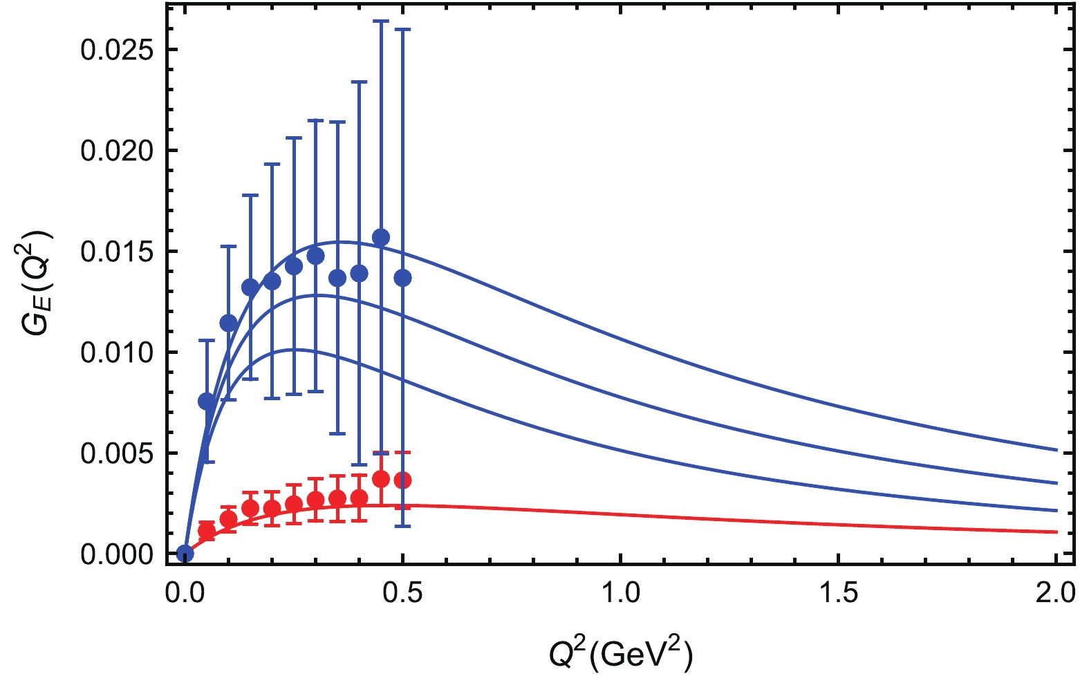
Figure 3. (color online) The sea quark contribution of u to the proton electric form factor versus momentum transfer
$Q^2$ . The three blue lines from top to bottom are for$\Lambda = $ 1.0, 0.9 and 0.8 GeV, respectively. The red line is the result for the strange quark with$\Lambda = 0.9$ GeV. The points with error bars are from lattice simulations [22].The d quark sea contribution to the proton electric form factor is plotted in Fig. 4. Similar to the u quark, the electric form factor first increases from 0 and then decreases with increasing
$ Q^2 $ . It can be clearly seen that the calculated sea quark contribution is larger than the lattice results. The larger sea contribution of the d quark than of the u quark is due to the fact that there is no intermediate octet contribution of the u quark, for which the only contribution is from the decuplet intermediate states. Similar results are found for the$ \bar{d}-\bar{u} $ asymmetry in the proton, where$ \bar{d} $ is in excess with respect to$ \bar{u} $ [38-41]. Although there is an obvious difference between the sea quark contributions of u and d, both are much larger than the strange quark contribution. The strange quark electric form factor is about 5-10 times smaller due to the suppression of the K meson loop.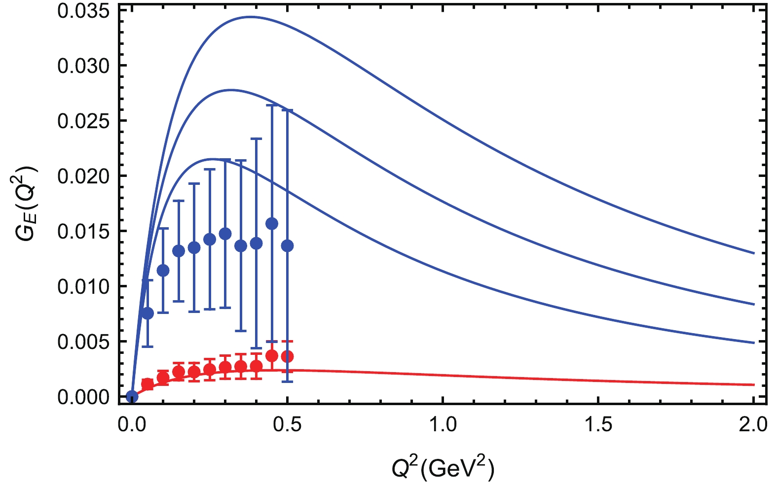
Figure 4. (color online) The sea quark contributions of d to the proton electric form factor versus momentum transfer
$Q^2$ . The three blue lines from top to bottom are for$\Lambda = $ 1.0, 0.9 and 0.8 GeV, respectively. The red line is the result for the strange quark with$\Lambda = 0.9$ GeV. The points with error bars are from lattice simulations [22].The sea contribution to the proton magnetic form factor of the u and d quarks with unit charge are plotted in Fig. 5 and Fig. 6. The calculated strange quark magnetic form factor is again in good agreement with the lattice results. All quark magnetic form factors increase monotonously with increasing
$ Q^2 $ . The absolute values of the u quark contribution are smaller than the lattice simulation results for the light quarks, while for the d quark contribution, the absolute values are larger than the lattice results. The absolute contributions of both u and d quarks are larger than of the strange quark, especially for small$ Q^2 $ . For$ Q^2 = 0 $ , the magnetic moments of the u and d sea quarks are$ -0.11 $ and$ -0.39 $ , respectively, while the strange quark magnetic moment is about$ -0.04 $ .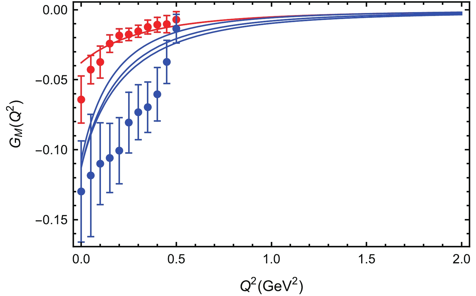
Figure 5. (color online) Same as Fig. 3 but for the magnetic form factor.
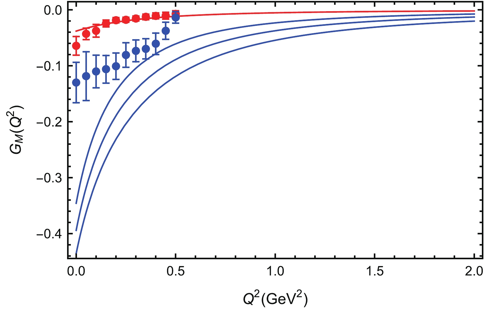
Figure 6. (color online) Same as Fig. 4 but for the magnetic form factor.
From the above figures, it can be seen that the u and d sea quark contributions are quite different. For both the electric and magnetic form factors, the absolute value of the d sea quark contribution is much larger than of u, because there are two up quarks and one down quark in a proton. The u quark in the loop diagram can only form a decuplet state and there is no intermediate octet contribution to the u sea quark form factors. We should mention that the difference between the light sea quark form factors is not due to the mass difference of u and d quarks. In fact, in our calculation the masses of
$ \pi^0 $ ,$ \pi^+ $ and$ \pi^- $ are degenerate. It is straightforward to see that the sea quark form factor of u (d) in the proton is the same as that of d (u) in the neutron, if the masses of proton and neutron are the same. The mass difference between proton and neutron leads to a small charge symmetry violation, i.e. a small difference between$ G^u_p $ and$ G^d_n $ ($ G^d_p $ and$ G^u_n $ ). The large difference between$ G^u_p $ and$ G^d_p $ is due to the effect of non-perturbative valence quark rather than of the mass difference between u and d.If the mass of the three u quark state is taken to be degenerate with respect to the nucleon mass, and the
$ \eta $ mass is taken to be degenerate with the$ \pi $ mass. the sea contribution of u and d quarks in the proton would be the same. This is an artifact of the present lattice simulations. Physically, three u quarks cannot form an octet baryon, and the mass of$ \eta $ is much larger than of$ \pi $ . Therefore, it would be very interesting and challenging to get the flavor asymmetry from the full lattice QCD simulations. -
In this work, we applied the nonlocal chiral effective Lagrangian to study the sea quark contribution of light quarks to the proton electromagnetic form factors. Since the sign of the u, d and s quark form factors are the same, this calculation helps to understand the experimental values of strange quark form factors. It is also interesting to compare our results with the lattice simulations. In our calculations, the parameter
$ \Lambda $ in the regulator is the same as in the lattice simulations, and was determined by fitting the nucleon form factors. The low energy constants$ c_1 $ and$ c_2 $ were determined from the experimental magnetic moments of the proton and neutron. Therefore, in calculating the sea quark form factors, there are no free parameters to be adjusted. Our results show that the electric form factors of light sea quarks with unit charge are positive, while the magnetic form factors are negative. Compared with the strange quark form factors, the absolute values of the light quark form factors are much larger. For both the electric and magnetic form factors, the contribution of the d quark is larger than of the u quark. The current lattice simulations for the light sea quark form factors are in between our results for u and d. Therefore, it would be interesting if this flavor asymmetry could be obtained from the full lattice QCD simulations.
Sea quark contributions to nucleon electromagnetic form factors with the nonlocal chiral effective Lagrangian
- Received Date: 2019-10-23
- Accepted Date: 2020-01-18
- Available Online: 2020-05-01
Abstract: The sea quark contributions to the nucleon electromagnetic form factors of the up, down and strange quarks are studied with the nonlocal chiral effective Lagrangian. Both octet and decuplet intermediate states are included in the one loop calculations. Compared with the strange quark form factors, although their signs are the same, the absolute value of the light quark form factors are much larger. For both the electric and magnetic form factors, the contribution of the d quark is larger than of the u quark. The current lattice simulations of the light sea quark form factors are in between our results for the u and d quarks.


 DownLoad: